| Issue |
A&A
Volume 708, April 2026
|
|
|---|---|---|
| Article Number | A137 | |
| Number of page(s) | 17 | |
| Section | Atomic, molecular, and nuclear data | |
| DOI | https://doi.org/10.1051/0004-6361/202556199 | |
| Published online | 03 April 2026 | |
Ionization equilibrium of nitrogen under kappa electron distributions
School of Nuclear Science and Technology, Lanzhou University,
Lanzhou
730000,
China
★ Corresponding authors: This email address is being protected from spambots. You need JavaScript enabled to view it.
; This email address is being protected from spambots. You need JavaScript enabled to view it.
Received:
1
July
2025
Accepted:
23
February
2026
Abstract
Non-Maxwellian electron energy distributions, such as kappa distributions, have been proposed to explain discrepancies in observed astrophysical plasmas. We employed the coronal approximation to study the level populations of ionized nitrogen under kappa distributions across a range of electron temperatures and densities. Both ground and metastable levels were considered. We propose a novel density diagnostic method that combines these level populations with spectroscopic measurements: level-resolved cross sections for key atomic processes – electron impact ionization, photoionization (PI), radiative recombination, and dielectronic recombination (DR) – are calculated using the level-to-level distorted wave method in the Flexible Atomic Code, generalized for kappa distributions, and the corresponding rate coefficients are then derived. Using these coefficients, we computed the ionization equilibrium, with a particular focus on the roles of DR and PI. We also investigated the suppression of DR by electron density and its influence on the resulting ionization equilibrium.
Key words: atomic data / atomic processes
© The Authors 2026
 Open Access article, published by EDP Sciences, under the terms of the Creative Commons Attribution License (https://creativecommons.org/licenses/by/4.0), which permits unrestricted use, distribution, and reproduction in any medium, provided the original work is properly cited.
This article is published in open access under the Subscribe to Open model. This email address is being protected from spambots. You need JavaScript enabled to view it. to support open access publication.
1 Introduction
The elemental abundances observed in astrophysical environments are shaped by stellar nucleosynthesis and the chemical evolution of galaxies, stars, and planets (Jonauskas 2022). Nitrogen (N), the fifth most abundant element in the Solar System and seventh in the Milky Way (Werbowy & Pranszke 2011; Cochran & Cochran 2002), exhibits a complex ionization behavior that is evident in its emission spectra in various charge states (Kewley & Dopita 2002; Denicoló et al. 2002; Shapley et al. 2015; Faisst et al. 2018; Martens et al. 2019). However, discrepancies in the intensities of solar transition region lines, particularly among isoelectronic sequences, suggest limitations in traditional modeling approaches under the coronal approximation (Hayes & Shine 1987; Judge et al. 1995; Curdt et al. 2001; Doschek & Mariska 2001; Del Zanna et al. 2002; Peter et al. 2014; Doschek et al. 2016; Polito et al. 2016; Dudík et al. 2017; Dufresne et al. 2023). In this regime, ionization and recombination occur on timescales much longer than those of excitation and deexcitation, enabling a decoupled treatment of ionization equilibrium and level populations (Dzifčáková et al. 2024).
In many studies, it is typically assumed that the electron energy distribution follows a Maxwellian distribution, which represents a plasma in thermal equilibrium. However, a growing body of observational and theoretical evidence demonstrates that a wide range of astrophysical environments exhibit non-Maxwellian characteristics, often featuring high-energy tails that deviate from thermal equilibrium. These nonequilibrium features are particularly evident in the solar wind, planetary magnetospheres, interstellar media, and photoionized nebulae (Livadiotis 2018; Pierrard & Lazar 2010; Zhang et al. 2013; Livadiotis & McComas 2013). Such distributions significantly alter the rates of atomic processes. One widely used model for describing suprathermal electron populations is the kappa distribution, which generalizes the Maxwellian distribution by introducing a high-energy power-law tail governed by the parameter κ. The kappa distribution is used to fit observations across a wide variety of astrophysical environments. This includes in situ measurements of particle distributions in planetary magnetic environments (Pierrard & Lemaire 1996; Mauk et al. 2004; Schippers et al. 2008; Xiao et al. 2008; Dialynas et al. 2009) and solar wind (Collier et al. 1996; Maksimovic et al. 1997a,b; Pierrard et al. 1999; Nieves & Viñas 2008; Le Chat et al. 2009; Pierrard 2012), as well as photon spectra of solar flare plasmas (Oka et al. 2013; Kašparová & Karlický 2009), emission line spectra of planetary nebulae (PNe) and galactic sources (Nicholls et al. 2012), and even the solar transition region (Dudík et al. 2011). Moreover, the kappa distribution can explain the abundance discrepancy problem in PNe (Nicholls et al. 2017). In the investigation of the PNe and H II regions, kappa distributions have successfully accounted for the systematic discrepancies between plasma diagnostics derived from collisionally excited lines and those obtained from recombination lines (Zhang et al. 2015; Lin & Zhang 2020). Kappa distributions have been utilized to examine the characteristic thermodynamic properties of energetic solar protons associated with an interplanetary coronal mass ejection and its resulting shock (Cuesta et al. 2024). Furthermore, the kappa distribution represents more than just a non-Maxwellian electron model; it identifies nonequilibrium plasmas, diagnoses acceleration sources, bridges micro-to-macro scales, embodies non-extensive statistics, and is essential for next-generation solar and astrophysical missions (Hahn & Savin 2015; Pierrard et al. 2023; Shen et al. 2023).
While several studies have explored kappa electron energy distributions (Dzifčáková et al. 2015, 2023, 2024; Song et al. 2025) and atomic processes involving N ions (Kim & Desclaux 2002; Jonauskas 2023; Kynienė et al. 2024; Defrance et al. 1985; Elizarov & Tupitsyn 2006; Crandall et al. 1978; Aichele et al. 1998; Song et al. 2024), few have fully integrated these effects into a unified model that simultaneously treats level populations and ionization balance. Building on the investigation of carbon ionization equilibrium by Dzifčáková et al. (2024), in this work we used the coronal approximation to investigate the level populations of ionized nitrogen under kappa electron distributions, explicitly accounting for both ground and metastable states. We computed level-resolved cross sections and rate coefficients for key atomic processes, including electron impact ionization (EII), photoionization (PI), radiative recombination (RR), and dielectronic recombination (DR), to evaluate their contributions to ionization equilibrium. Special attention was paid to the suppression of DR by electron density, a factor often neglected in earlier studies.
The structure of the paper is as follows: Section 2 describes the theoretical framework and the modeling approach. Section 3 presents the results and analysis. Section 4 summarizes our conclusions.
2 Methods
As mentioned in Sect. 1, we calculated the level populations, rate coefficients, and ionization equilibrium of N under the coronal approximation, taking the metastable states into account. In this section, we provide a detailed explanation of our calculation methods.
2.1 Non-Maxwellian electron kappa distributions
We characterized the electron energy distributions using the well-known kappa distributions, a family of non-Maxwellian distributions that exhibit an increased number of particles in the high-energy tail, as described by the thermodynamic index κ:
 (1)
(1)
where  ; ϵ and Te represent the electron energy and temperature, respectively; kB is the Boltzmann constant, i.e., 1.38 × 10⁻²³ J/K; and Aκ is the normalization constant that approaches 1 when κ → ∞, which can be expressed as
 (2)
(2)
Here, κ is a parameter that describes the degree to which the distribution departs from an equilibrium Maxwellian distribution. A smaller value of κ is associated with a greater deviation from the Maxwellian distribution. In the limit as κ → ∞, the distribution reverts to the standard Maxwellian distribution,
 (3)
(3)
A family of normalized κ energy distributions is shown in Fig. 1, together with a Maxwellian distribution. As κ → ∞, the distribution reduces to the Maxwellian; lower values of κ represent increasingly significant high-energy enhancements. Some observations of space plasma have revealed an empirical separation of the κ spectrum (Livadiotis & McComas 2013), which is divided into near- and far-equilibrium regions, with a separatrix at κ = 2.5. The indices in the range 2.5 < κ ≤ ∞ (Dialynas et al. 2009) represent the near-equilibrium region, while the far-equilibrium region has indices 1.5 < κ ≤ 2.5 (Livadiotis & McComas 2011a,b). Moreover, the introduction of different values of κ provides a reasonable explanation for the contradictory phenomena observed in experiments. In the very early phase of a solar flare, if κ = 2 (or even lower) is adopted, the non-Maxwellian high-energy tail causes the temperature diagnosed by line ratios of Fe to be nearly twice as high as the Maxwellian temperature retrieved from Geostationary Operational Environmental Satellites (GOES) X-rays, thereby addressing the previously noted systematic discrepancy between the two (Dzifčáková et al. 2018). When the Sun is in an active region, κ ≤ 3 values are necessary to replicate the observed Fe line ratios (Lörinčík et al. 2020). Moreover, at log Te = 5.9 K, κ = 5 provides an excellent match to the observed  line intensity ratio, while for Si, κ = 7 successfully fits the experimental measurements (Dzifčáková & Dudík 2013). Regarding the temperature and metallicity discrepancies between the H II regions and the PNe arising from divergent measurement techniques, the energy distribution does not need to deviate significantly from equilibrium, and κ > 10 is adequate to encompass virtually all observed objects (Nicholls et al. 2012).
Based on the demonstrated success of the values of κ in astrophysical phenomena, we performed calculations for κ = 2, 3, 5, and 10 to investigate the influence of the κ distributions on the level populations and the ionization equilibrium of N.
 |
Fig. 1 Comparison of the Maxwellian distribution and κ distributions at a temperature of 1.16 × 10⁵ K. Different colors represent the different energy distributions. |
2.2 Level populations
In the collisional radiative model, the population of each excited level is described by the following differential rate equation:
 (4)
(4)
where Ni and Ne represent the population of the i-th level and the electron density, respectively. The Aij are the probabilities of a radiative transition; Sij are the EII rate coefficients; Rij are the recombination rate coefficients; and Qij and Qji correspond to the electron impact excitation and deexcitation rate coefficients, respectively. The ionization, recombination, and excitation rate coefficients can be derived by convoluting the corresponding cross sections, which are calculated using the distorted-wave method in conjunction with the electron energy distribution function. Specifically, the deexcitation cross sections are computed based on the principle of detailed balance, i.e.,
 (5)
(5)
where  and
and  are cross sections for deexcitation and excitation, respectively; ωi represents the statistical weight of level i, which is equal to 2Ji + 1, and Ji is the total angular momentum of level i; and ∆Eij is the energy difference between the i-th and j-th levels. The ground and excited states considered in the excitation and deexcitation processes are listed in Table 1.
In the quasi-steady-state approximation, the level population does not change over time, i.e.,  . Level populations should satisfy the normalization condition, that is,
  , where r represents the total number of ground and excited levels. Moreover, in the corona approximation, the ionization and recombination terms can be removed because of the low electron density. Equation (4) can be rewritten as follows:
 (6)
(6)
Ground and excited states included in the calculations of excitation and deexcitation rate coefficients.
2.3 Rate coefficients
Based on the coronal approximation, we derived the total cross sections from the populations of ground and metastable levels, that is,
 (7)
(7)
where σtotal (ϵ) and  represent the total cross sections and the partial cross sections of each ground level and metastable level, respectively; and r denotes the total number of energy levels. The rate coefficients were calculated via direct numerical integration over electron energy distributions,
 (8)
(8)
where v(ϵ) is the relativistic electron velocity, I0 is the threshold, and fe (ϵ, Te) represents the distribution of electron energy.
In particular, it should be emphasized that the PI process is independent of the electron distribution and depends solely on the radiation field. Thus, the PI rate is calculated using the expression (Nussbaumer & Storey 1975; Dzifčáková et al. 2024):
 (9)
(9)
where σphot is the PI cross section, Jλ is the mean intensity, λ is the wavelength and λ0 is the threshold wavelength, h is the Planck constant, and c is the speed of light. The mean disk intensity was obtained from the solar minimum irradiances of Woods et al. (2009), assuming no limb brightening. We note that Rphot depends on the ambient radiation field and is independent of κ. However, it does vary with the distance (r) above the solar surface through the dependence of Jλ on the dilution factor W(r), where Jλ = W(r)Īλ. Here, Īλ is the disk-averaged radiance at wavelength λ (Dzifčáková et al. 2024).
In addition, for the DR process, the Maxwellian rate coefficient can be expressed as (Behar et al. 1999)
 (10)
(10)
Here, me denotes the electron mass; gi and gj are the statistical weights of the initial state (i) and the doubly excited autoionization state (j), respectively; and  and
and  represent the Auger decay rate and radiative transition branching ratio of the doubly excited level (j), respectively. As stated in Sect. 2.1, a κ distribution can be expressed as a linear combination of Maxwellian distributions (Hahn & Savin 2015), i.e.,
 (11)
(11)
where fM(ϵ, ajTκ) is the Maxwellian energy distribution at a temperature of TM = ajTκ. Therefore, the DR rate coefficients for a κ distribution can be derived from the Maxwellian rate given by Eq. (10). The coefficients cj and aj were obtained from Hahn & Savin (2015).
2.4 Ionization equilibrium
The ionization state can be determined using the following collisional equations:
![Mathematical equation: $\displaylines{{{d{N^z}} \over {dt}} = \left( {{N_e}S_e^{z - 1 \to z} + S_p^{z - 1 \to z}} \right){N^{z - 1}} - [{N_e}\left( {S_e^{z \to z + 1} + {R^{z \to z - 1}}} \right) \cr + S_p^{z \to z + 1}]{N^z} + {N_e}{R^{z + 1 \to z}}{N^{z + 1}}, \cr} $](/articles/aa/full_html/2026/04/aa56199-25/aa56199-25-eq21.png) (12)
(12)
where Nz represents the populations of each charge state (z). The terms  and
and  denote the EII rate coefficients for the transitions from charge state z − 1 to z and from z to z + 1, respectively.
  and
and  denote the PI rate for the transitions from the charge state z − 1 to z and from z to z + 1, respectively. Similarly, Rz→z−1 and Rz+1→z represent the total recombination rate coefficients for the transitions from the charge state z to z − 1 and from z + 1 to z, respectively. For the ionization processes, we took both EII and PI into account. For the recombination processes, we considered both RR and DR. By solving the collisional equations in a steady state, where the time derivative of the ion population is zero, i.e.,
  , we can derive the following equation:
 (13)
(13)
where αEII, αRR, and αDR represent the rate coefficients for the EII, RR, and DR processes, respectively; and αPI denotes the rate of the PI process.
Dielectronic recombination is a multistep process in which an incoming free electron is captured by an ion, exciting one of the bound electrons and producing a doubly excited resonance state. The DR process is considered complete when the recombined ion stabilizes to a bound state through the radiative decay of either the core or the Rydberg electron. An ion left in a Rydberg state is particularly susceptible to reionization through collisions with free electrons, especially in high-density plasma environments. Under these conditions, the DR process is significantly suppressed, and the rate coefficients can be expressed as (Dzifčáková et al. 2024)
 (14)
(14)
where RDR (Te) represents the DR rate in the zero density limit. The suppression factor (SF), S (Ne, Te, q, M), is dimensionless. It depends on the electron density (Ne), the temperature (Te), the isoelectronic sequence (M), and the parameter (q), which is specific to the ion. Nikolić et al. (2013, 2018) provided fits for the SF under a Maxwellian distribution, which were subsequently extended to kappa distributions (Dzifčáková et al. 2023; Hahn & Savin 2015):
 (15)
(15)
where SM(Ne, Tj, q, M) represents the SF for the Maxwellian distribution, and aj denotes the coefficients used in the approximation of a kappa distribution as a sum of several Maxwellians at varying temperatures (Tj). Specifically, the unsuppressed DR rates were first computed using the level-to-level distorted-wave (LLDW) method. The suppressed DR rates were then derived from these unsuppressed rates using the analytic SF.
We calculated the relevant cross sections using the LLDW method, which is implemented in the Flexible Atomic Code (FAC; Gu 2008). The other data presented in this work, including level populations, spectra, rate coefficients, ionization equilibrium, and density suppression, were calculated using our custom program written in Python.
Ground and metastable levels considered in this work.
3 Results and discussion
This section presents the calculated level populations and their implications for density and temperature diagnostics. The levels included in our calculations are presented in Table 2. It is important to note that for the neutral N atom, there are no long-lived metastable states; therefore, we only considered the five ground levels in our investigation.
3.1 Level population
Figure 2 depicts the dependence of the level populations of N I through N IV on the electron density for both kappa and Maxwellian distributions. For N I, it is evident that, at a given temperature of 104.1 K, the populations of its five ground levels exhibit negligible variation with increasing electron density, remaining essentially constant. The population of the lowest level (2s22p3 4S3/2) is approximately 0.86 and dominates across the entire density range, i.e., from 107 to 1013 cm−3. The populations of the other four levels are all below 0.1. Moreover, for N I, the variations in the level populations with density are almost identical in the kappa and Maxwellian electron energy distributions. For N II, the populations of the four lowest ground levels and one metastable level (2s12p3 5S2) remain nearly constant with increasing density. For the kappa distribution with κ = 2, their populations are approximately 0.54, 0.20, 0.12, 0.15, and 0.09, respectively. However, the population of 2s22p2 1S0 continues to increase with increasing density until the electron density reaches about 1010 cm−3. When the density increases from 107 cm−3 to 1010 cm−3, its population grows by two orders of magnitude, yet it remains negligibly small. Beyond this density, i.e., 1010 cm−3, the population of this level stabilizes and does not change significantly with increasing density. Moreover, for levels 2s22p2 1S0 and 2s12p3 5S2, the populations under the κ = 2 kappa distribution are slightly larger than those under the Maxwellian distribution. For N III, the populations of the ground state levels, 2s22p1 2P1/2 and 2s22p1 2P3/2, exhibit minimal variation with increasing electron density when the density is below 1010 cm−3. When the electron density exceeds this value, the populations of these two levels decrease slightly with increasing density. For the kappa distribution with κ = 2, their populations decrease approximately from 0.58 to 0.43 and from 0.40 to 0.29, respectively. For metastable levels, the population increases with density when the density is below 1010 cm−3. However, the populations remain dominated by the two ground levels. At this density, i.e., 1010 cm−3, the hierarchy of the three metastable populations is inverted, with level 2s12p2 4P1/2 becoming the most populated one. For the lowest ground level (2s22p1 2P1/2), the population under a kappa distribution is slightly higher than that under the Maxwellian distribution, whereas for the other levels the opposite trend is observed. For N IV, the population of 2s2 1S0 decreases from 0.87 to 0.68 with increasing density above 109 cm−3, whereas the other levels show the opposite trend. For the ground level 2s2 1S0, the population is virtually identical under both the kappa and Maxwellian distributions. However, for the other levels, the Maxwellian population is slightly higher than that of the kappa distribution. For higher-charge-state N ions, the level populations remain virtually unchanged with density, and the ground level population is extremely close to unity. This trend is also evident in the subsequent discussion of rate coefficients; for this reason, these results are not presented extensively in this section.
Similarly, the evolution of the level populations of N I through N IV as a function of electron temperature is presented in Fig. 3. The selected electron density is 1011 cm−3. The results were calculated for kappa distributions with κ values of 2, 3, 5, and 10, in addition to the Maxwellian distribution. For N I, the population of level 2s22p3 4S3/2 is seen to drop steeply with rising temperature, declining from 0.85 to 0.37 when the temperature increases from 104.1 K to 105 K at an electron density of 1011 cm−3. Conversely, the populations of all other levels increase. At a temperature of 2.3 × 10⁴ K, the populations of levels 2s22p3 2D5/2 and 2s22p3 2P1/2 cross over. Only at relatively high temperatures do the populations of the four levels, i.e., 2s22p3 2D5/2, 2s22p3 2D3/2, 2s22p3 2P1/2, and 2s22p3 2P3/2, exceed 0.1 and thereby influence the overall populations; their contributions are negligible in the low-temperature regime. Moreover, the temperature dependence of the level populations is almost identical for the kappa and Maxwellian distributions. For N II, a similar trend to that of N I is observed. The population of the ground level 2s22p2 3P0 decreases with increasing electron temperature. Under a κ = 2 distribution, the population decreases from 0.64 to 0.40. Moreover, the populations of levels 2s22p2 1D2, 2s22p2 1S0, and 2s12p3 5S2 rise with increasing temperature. Levels 2s22p2 3P0, 2s22p2 3P1, and 2s22p2 3P2 dominate the population variation of N II ion. For N III, the population of the ground level 2s22p1 2P1/2 decreases, while that of the level 2s22p1 2P3/2 increases with the temperature. Moreover, the populations under the kappa distribution and the Maxwellian distribution remain essentially the same. For the metastable levels, i.e., 2s12p2 4P1/2, 2s12p2 4P3/2, and 2s12p2 4P5/2, all populations increase with increasing electron temperature. For N IV, the population of level 2s2 1S0 decreases gradually as the temperature rises. At a density of 1011 cm−3, its population decreases from 0.99 to 0.63. Moreover, the populations of all other levels grow with temperature. At relatively low temperatures, the ground state dominates. However, as the temperature increases, the metastable levels begin to exert a significant influence on the total population distribution. For N V and higher-charge nitrogen ions, the level populations are dominated almost entirely by the lowest ground level and are very close to unity; therefore, we do not show their temperature dependence in Fig. 3.
The results of level populations show that the population of metastable levels changes by orders of magnitude with increasing electron density and temperature. For example, for N III, the population of metastable levels 2s12p2 4P1/2, 2s12p2 4P3/2, and 2s12p2 4P5/2 changes by an order of magnitude with increasing electron density, as presented in Fig. 2. Moreover, when the temperature increases from 104 to 105 K, the metastable levels also increase by an order of magnitude. These findings provide guidance for density and temperature diagnostics that use the spectrum between these levels. The relative intensity of the spectrum can be expressed as follows:
 (16)
(16)
where j > i and Nj is the population of the upper energy level involved in the transition, Aij denotes the transition rate from level j to level i, and Φ(λ) represents the broadening function. Since Aij is constant for a given transition, the spectral intensity depends solely on the upper level population, Nj.
Figure 4 presents the N III spectrum calculated at different electron densities for the transition from 2s12p2 to 2s22p1. In Fig. 4, the four peaks from left to right correspond to the transitions from 2s12p2 4P1/2 to 2s22p1 2P3/2, from 2s12p2 4P3/2 to 2s22p1 2P3/2, from 2s12p2 4P5/2 to 2s22p1 2P3/2, and from 2s12p2 4P1/2 to 2s22p1 2P1/2. The corresponding transition rates (Aij) are 54.84 s−1, 23.29 s−1, 106.45 s−1, and 154.29 s−1, respectively. When taking the level populations under different densities into account, the intensity relationships of these four peaks change. However, for each transition, Aij remains constant, so intensity variations directly reflect population changes. Thus, for a particular peak in Fig. 4, the intensity at different densities is directly proportional to the level population at that density.
We calculated the ratios of the two satellite lines of the spectrum corresponding to the lower level 2s22p1 2P3/2 of N III, namely  (designated as R1) and
  (designated as R2), and examined their variations with electron density and temperature. The results are presented in Figs. 5 and 6, respectively, which show that the satellite line ratios change significantly with increasing density and temperature. For the kappa distribution with κ = 2, when the density increases from 107 cm−3 to 1013 cm−3, the ratio of the first set of satellite lines (R1) increases from 0.15 to 1.51. Meanwhile, the other ratio (R2) decreases from 0.85 to 0.32, a 62.4% reduction. Moreover, when the temperature increases from 104 K to 105 K, R1 decreases from 1.51 to 1.14, a considerable reduction of 24.5%. Given the sensitivity of the level population of N III to density and temperature variations, plasma conditions in astrophysical environments can be inferred from the spectral intensity, thus achieving the purpose of density diagnosis.
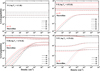 |
Fig. 2 Level populations of N I, N II, N III, and N IV as a function of electron density. The numbers 00, 01, 02, etc., refer to the energy levels listed in Table 2. Different colors represent different electron energy distributions. |
 |
Fig. 3 Level populations of N I, N II, N III, and N IV as a function of temperature. The numbers 00, 01, 02, etc., refer to the energy levels listed in Table 2. The selected electron density is 1011 cm−3. Different colors indicate different electron energy distributions. |
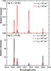 |
Fig. 4 Spectrum of N III, with the transition from 2s12p2 to 2s22p1. Different colors correspond to different densities. |
 |
Fig. 5 Dependence of the spectral intensity ratio of N III on electron density. The double-dot-dashed line represents the ratio of the transition intensity from 2s12p2 4P1/2 to 2s22p1 2P3/2 to that from 2s12p2 4P5/2 to 2s22p1 2P3/2 (R1). The dashed line represents the ratio of the transition intensity from 2s12p2 4P3/2 to 2s22p1 2P3/2 to that from 2s12p2 4P5/2 to 2s22p1 2P3/2 (R2). Different colors correspond to different energy distributions. |
 |
Fig. 6 Dependence of the spectral intensity ratio of N III on electron temperature. The meanings of the different lines are the same as in Fig. 5. |
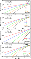 |
Fig. 7 DI and EA rate coefficients of N I and N II. Different colors correspond to different energy distributions, and the different line shapes represent different electron densities. |
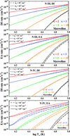 |
Fig. 8 DI and EA rate coefficients of N III and N IV. Different colors correspond to different energy distributions, and the different line shapes represent different electron densities. |
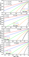 |
Fig. 9 DI and EA rate coefficients of N V, as well as the EA rate coefficients of N VI and N VII. Different colors correspond to different energy distributions, and the different line shapes represent different electron densities. |
 |
Fig. 10 PI rate of nitrogen. Different colors correspond to different ions, and the different line shapes represent different electron densities. |
 |
Fig. 11 DR rate coefficients of N I. Different colors correspond to different energy distributions, and the different line shapes represent different electron densities. |
 |
Fig. 12 DR and RR rate coefficients of N II to N VII. Different colors correspond to different energy distributions, and the different line shapes represent different electron densities. |
3.2 Rate coefficients
In this subsection, we discuss the rate coefficients of the various atomic processes we calculated in detail, including ionization and recombination. The EII rate coefficients from N I to N VII calculated using both kappa and Maxwellian distributions, at selected electron densities of 107 cm−3, 109 cm−3, and 1011 cm−3, are illustrated in Figs. 7 to 9. The rate coefficients include contributions from both direct ionization (DI) and excitation-autoionization (EA) processes. These results indicate that the DI rate coefficients are approximately one or two orders of magnitude higher than those of the EA processes, except for N I. For N I, the contribution from the EA process is comparable to that of the DI process. Given the relatively low temperatures adopted in our calculations, the ionization rate coefficients increase with temperature and the rate coefficients increase with decreasing κ (i.e., as the distribution deviates more significantly from the equilibrium Maxwellian distribution). This trend can be attributed to the greater number of particles encompassed by the kappa distribution, which is consistent with the low-energy region depicted in Fig. 1. For N III and N IV ions, the level populations within the temperature range we investigated are strongly density-dependent: the metastable level populations rise markedly with increasing density. The increase in the metastable population raises the total ionization cross sections, which depend on the populations, so the ionization rate corresponds to increases in density. Consequently, the ionization rate coefficients computed at the three densities, i.e., 107 cm−3, 109 cm−3, and 1011 cm−3, differ substantially, most notably for the EA channel of N IV. In contrast, the ionization rate coefficients of all other ions remain essentially identical across the density grid. It should be noted that the EA cross sections for N VI and N VII are both exactly zero, so their corresponding rate coefficients vanish and are therefore omitted from Fig. 9. In addition, to benchmark our calculated ionization rate coefficients, taking N II and N III as examples, we compare our calculations with the KAPPA database (Dzifčáková et al. 2021) in Figs. A.1 and A.2. A discussion of the comparison results is also given in the appendix.
In addition to EII, the PI rate was examined. We used Eq. (9) to calculate the PI rate of N, and the results are presented in Fig. 10. Note that the PI rate depends only on the radiation field intensity and the level populations, and thus the PI rate varies with temperature and density exactly the same way as the level populations. Furthermore, we observe that the PI rate decreases systematically as the charge state increases.
In addition to the ionization process, we investigated the influence of the electron energy distribution on the recombination rate coefficients – both RR and DR. Figures 11 to 13 present the rate coefficients for these recombination processes. Since the RR cross sections for N I ion are both exactly zero, only the DR rate coefficients are shown separately in Fig. 11. As can be seen, because the RR cross sections decrease steadily with the incident electron energy, their rate coefficients likewise diminish as the temperature rises. In contrast, the temperature dependence of the DR rate coefficients is more intricate. Over the temperature range we investigated, the DR rate coefficients exceed the RR rate coefficients for all ions except N VI and N VII for both kappa and Maxwellian distributions. In addition, for N III, the RR rate coefficients become slightly larger than the DR rate coefficients at the lowest temperatures. Moreover, the density dependence of the RR rate coefficients simply tracks that of the level populations and does not need to be repeated here. For the DR process, however, its rate coefficients are suppressed by higher densities: the higher the density, the stronger the suppression. Thus, the DR rate coefficients decrease markedly as the density increases from 109 cm−3 to 1011 cm−3. Specifically, for a given energy distribution and temperature, the rate coefficients of the DR process decrease as the electron density increases. The total recombination rate coefficients are presented in Fig. 13, where it is evident that they are also strongly affected by the electron density due to the density suppression of the DR process, except for N VI and N VII, for which the total recombination process is governed by the RR process.
Similarly, to validate the accuracy of our calculations, we compared the RR rate coefficients calculated for all N ions with those from the Atomic Data and Analysis Structure (ADAS) database (Summers & O’Mullane 2011) and the FLYCHK code (Chung et al. 2005). The comparison is presented in Fig. A.3. Furthermore, taking N II and N III as examples, we also compared the total recombination rates calculated in this work with those from the KAPPA database (Summers & O’Mullane 2011). The results are shown in Figs. A.4 and A.5. A detailed discussion of these comparison results is also provided in the appendix.
 |
Fig. 13 Total recombination rate coefficients of N II to N VII. Different colors correspond to different energy distributions, and the different line shapes represent different electron densities. |
3.3 Ionization equilibrium
Armed with these accurate, level-resolved rate coefficients, we evaluated the ionization equilibrium of N ions. We first considered the EII, RR, and DR processes without density suppression to compute the ionization equilibrium of nitrogen under different electron energy distributions at selected electron densities of 107 cm−3, 109 cm−3, and 1011 cm−3, as shown in Fig. 14. The results demonstrate that the greater the deviation from the equilibrium Maxwellian distribution, the more pronounced the differences in the ionization equilibrium become. For the case of κ = 2, within the entire temperature range investigated (104 to 106 K), neutral nitrogen and N II ion have negligible fractional abundances. Even at 104 K, the ion population is already dominated by N III and N IV. As κ increases and the distribution approaches the Maxwellian form, lower charge states become increasingly populated. Under a Maxwellian distribution, the fractional abundance of neutral nitrogen reaches 0.947 at 104 K. This difference arises because, at low temperatures, the EII rate coefficients for κ = 2 are significantly higher than those for the Maxwellian distribution, enhancing ionization from lower charge states and shifting the ionization equilibrium toward higher ionization stages. In addition, the effect of electron density on the ionization equilibrium is minimal, with only slight changes observed for N III, N IV, and N V. The influence of temperature and density on the ionization equilibrium is generally less pronounced than that of the electron energy distribution.
As discussed in Sect. 2.4, the increase in electron density suppresses the DR process to some extent. We computed the density SF taking N II as an example by using Eqs. (14) and (15), at electron densities of 107 cm−3 and 1011 cm−3; the results are presented in Fig. B.1.
After incorporating the density suppression effect for the DR process, we recalculated the ionization equilibrium of N, as shown in Fig. 15. Taking a density of 1011 cm−3 as an example, it can be observed that the density suppression effect has a very strong influence on the ionization equilibrium of nitrogen. Furthermore, the results reveal that suppression of DR reduces the overall recombination rate, thus causing the peak of ionization equilibrium to shift toward lower temperatures both for kappa and Maxwellian distributions. This shift is most pronounced for lower-charge-state N ions.
Furthermore, we analyzed the influence of the PI process on the ionization equilibrium, as shown in Fig. 16. The PI process significantly influences the ionic distribution only at low temperatures and for the lower charge states, whereas it has virtually no effect on the distribution of N III and higher-charged N ions. This effect becomes increasingly pronounced as κ increases, that is, as the electron distribution approaches the Maxwellian distribution. However, in any case, neither density suppression nor PI has an impact on the ionization balance of nitrogen comparable to that of the adopted electron energy distribution.
In Fig. 17, we present the final ionization equilibrium of N when all processes, namely EII, PI, RR, and suppressed DR, are taken into account. The ionization equilibrium for N we calculated is compared with the KAPPA database (Dzifčáková et al. 2021), as shown in Fig. 18. We can observe that, overall, our distributions are shifted toward lower temperatures, which is due to the fact that we accounted for the density suppression of DR in our calculations.
 |
Fig. 14 Ionization equilibrium of N at three different electron densities, including the effects of EII, RR, and DR processes without density suppression. Different colors correspond to different charge states, and the different line shapes represent different electron densities. |
 |
Fig. 15 Ionization equilibrium of N, incorporating the influence of density suppression at a density of 1011 cm−3. Different colors correspond to different charge states. The solid lines denote the ionization equilibrium obtained with the density suppression effect included, whereas the dashed lines show the results without this suppression effect. |
 |
Fig. 16 Influence of the PI process on the ionization equilibrium of nitrogen. Different colors correspond to different charge states, and the selected density is 1011 cm−3. The solid lines represent calculations that include the PI process, and the dashed lines correspond to those without it. |
 |
Fig. 17 Final ionization equilibrium of nitrogen including all atomic processes, namely EII, PI, RR, and suppressed DR. Different colors correspond to different charge states, and the different line shapes represent different electron densities. |
 |
Fig. 18 Comparison of the ionization equilibrium for N from our calculations and KAPPA (Dzifčáková et al. 2021) at a density of 107 cm−3. Different colors correspond to different charge states. |
4 Summary and conclusions
We have carried out a comprehensive study of the level populations, rate coefficients, and ionization equilibrium of nitrogen ions in plasmas characterized by the kappa distribution, a non-Maxwellian electron energy distribution function commonly found in astrophysical environments. For ionization stages ranging from N II to N VII, our analysis includes both ground states and long-lived metastable levels. Our results demonstrate that metastable level populations are highly sensitive to variations in electron temperature and density. Based on these dependences, we propose a novel diagnostic approach that combines level population modeling with spectroscopic observations to infer plasma conditions.
We further computed level-resolved rate coefficients for key atomic processes, including EII, PI, RR, and DR, under both Maxwellian- and kappa-distributed electron energies. Using these rates, we determined the resulting ionization equilibrium of nitrogen ions, finding that non-Maxwellian effects have a strong influence. Our analysis reveals that PI and density suppression for DR play significant roles in shaping the ionization equilibrium. These processes, especially under kappa distribution conditions, can substantially shift the ionization equilibrium toward higher or lower charge states, depending on the temperature, density, and the value of κ.
Dzifčáková et al. (2024) investigated the ionization equilibrium of carbon under a κ distribution, and our results are similar to their findings in several regards. First, we find that level-resolved ionization rates increase with density (e.g., for N IV), whereas the total recombination rate decreases, and that recombination processes shift the formation temperatures of lower-charge-state ions toward lower values. These trends were also reported by Dzifčáková et al. (2024) for carbon. Second, both studies show that as κ decreases (i.e., as the distribution departs further from a Maxwellian distribution), the ion formation temperature decreases markedly, the temperature range over which the ion forms becomes broader, and the peak abundance declines. Finally, both studies find that the influence of density suppression on the ionization balance weakens as κ decreases, and that the PI process is significant only at relatively high κ values.
These findings provide new insights into the ionization equilibrium of nitrogen in non-Maxwellian plasmas, contributing to a more accurate interpretation of astrophysical and laboratory plasma diagnostics.
Acknowledgements
We acknowledge support from the China National Natural Science Foundation Grant No. 12374231.
References
- Aichele, K., Hartenfeller, U., Hathiramani, D., et al. 1998, J. Phys. B: At. Mol. Opt. Phys., 31, 2369 [Google Scholar]
- Behar, E., Mandelbaum, P., & Schwob, J. L. 1999, Phys. Rev. A, 59, 2787 [Google Scholar]
- Chung, H. K., Chen, M. H., Morgan, W. L., Ralchenko, Y., & Lee, R. W. 2005, HEDP, 1, 3 [Google Scholar]
- Cochran, A. L., & Cochran, W. D. 2002, Icarus, 157, 297 [NASA ADS] [CrossRef] [Google Scholar]
- Collier, M., Hamilton, D., Gloeckler, G., Bochsler, P., & Sheldon, R. 1996, Geophys. Res. Lett., 23, 1191 [NASA ADS] [CrossRef] [Google Scholar]
- Crandall, D. H., Phaneuf, R. A., & Taylor, P. O. 1978, Phys. Rev. A, 18, 1911 [Google Scholar]
- Cuesta, M., Cummings, A., Livadiotis, G., et al. 2024, ApJ, 973, 76 [Google Scholar]
- Curdt, W., Brekke, P., Feldman, U., et al. 2001, A&A, 375, 591 [NASA ADS] [CrossRef] [EDP Sciences] [Google Scholar]
- Defrance, P., Chantrenne, S., Brouillard, F., et al. 1985, Nucl. Instrum. Methods Phys. Res. B, 9, 400 [Google Scholar]
- Del Zanna, G., Landini, M., & Mason, H. E. 2002, A&A, 385, 968 [NASA ADS] [CrossRef] [EDP Sciences] [Google Scholar]
- Denicoló, G., Terlevich, R., & Terlevich, E. 2002, MNRAS, 330, 69 [CrossRef] [Google Scholar]
- Dialynas, K., Krimigis, S., Mitchell, D., et al. 2009, J. Geophys. Res. Space Phys., 114, A01212 [Google Scholar]
- Doschek, G. A., & Mariska, J. T. 2001, ApJ, 560, 420 [NASA ADS] [CrossRef] [Google Scholar]
- Doschek, G. A., Warren, H. P., & Young, P. R. 2016, ApJ, 832, 77 [NASA ADS] [CrossRef] [Google Scholar]
- Dudík, J., Dzifčáková, E., Karlicky, M., & Kulinová, A. 2011, A&A, 529, A103 [NASA ADS] [CrossRef] [EDP Sciences] [Google Scholar]
- Dudík, J., Polito, V., Dzifčáková, E., Del Zanna, G., & Testa, P. 2017, ApJ, 842, 19 [CrossRef] [Google Scholar]
- Dufresne, R. P., Del Zanna, G., & Mason, H. E. 2023, MNRAS, 521, 4696 [NASA ADS] [CrossRef] [Google Scholar]
- Dzifčáková, E., & Dudík, J. 2013, ApJS, 206, 6 [CrossRef] [Google Scholar]
- Dzifčáková, E., Dudík, J., Kotrč, P., Fárník, F., & Zemanová, A. 2015, ApJS, 217, 14 [CrossRef] [Google Scholar]
- Dzifčáková, E., Zemanová, A., Dudík, J., & Mackovjak, v. 2018, ApJ, 853, 158 [Google Scholar]
- Dzifčáková, E., Dudík, J., Zemanová, A., Lörinčík, J., & Karlický, M. 2021, ApJS, 257, 62 [CrossRef] [Google Scholar]
- Dzifčáková, E., Dudík, J., Pavelková, M., Solarová, B., & Zemanová, A. 2023, ApJS, 269, 45 [CrossRef] [Google Scholar]
- Dzifčáková, E., Dufresne, R. P., Dudík, J., & Del Zanna, G. 2024, A&A, 690, A340 [NASA ADS] [CrossRef] [EDP Sciences] [Google Scholar]
- Elizarov, A. Y., & Tupitsyn, I. I. 2006, J. Phys. B: At. Mol. Opt. Phys., 39, 1395 [Google Scholar]
- Faisst, A. L., Masters, D., Wang, Y., et al. 2018, ApJ, 855, 132 [NASA ADS] [CrossRef] [Google Scholar]
- Gu, M. 2008, Can. J. Phys., 86, 675 [NASA ADS] [CrossRef] [Google Scholar]
- Hahn, M., & Savin, D. 2015, ApJ, 809, 178 [NASA ADS] [CrossRef] [Google Scholar]
- Hayes, M., & Shine, R. A. 1987, ApJ, 312, 943 [NASA ADS] [CrossRef] [Google Scholar]
- Jonauskas, V. 2022, A&A, 659, A11 [NASA ADS] [CrossRef] [EDP Sciences] [Google Scholar]
- Jonauskas, V. 2023, MNRAS, 526, 2104 [Google Scholar]
- Judge, P. G., Woods, T. N., Brekke, P., & Rottman, G. J. 1995, ApJ, 455, L85 [NASA ADS] [Google Scholar]
- Kašparová, J., & Karlický, M. 2009, A&A, 497, L13 [NASA ADS] [CrossRef] [EDP Sciences] [Google Scholar]
- Kewley, L. J., & Dopita, M. A. 2002, ApJS, 142, 35 [Google Scholar]
- Kim, Y., & Desclaux, J. P. 2002, Phys. Rev. A, 66, 012708 [NASA ADS] [CrossRef] [Google Scholar]
- Kynienė, A., Masys, v., & Jonauskas, V. 2024, J. Quant. Spectrosc. Radiat. Transfer, 315, 108898 [Google Scholar]
- Le Chat, G., Issautier, K., Meyer-Vernet, N., et al. 2009, Phys. Plasmas, 16, 102903 [CrossRef] [Google Scholar]
- Lin, B., & Zhang, Y. 2020, ApJ, 899, 33 [Google Scholar]
- Livadiotis, G. 2018, Universe, 4, 144 [Google Scholar]
- Livadiotis, G., & McComas, D. 2011a, ApJ, 738, 64 [Google Scholar]
- Livadiotis, G., & McComas, D. J. 2011b, ApJ, 741, 88 [NASA ADS] [CrossRef] [Google Scholar]
- Livadiotis, G., & McComas, D. J. 2013, Space Sci. Rev., 175, 183 [Google Scholar]
- Lörinčík, J., Dudík, J., Zanna, G., Dzifčáková, E., & Mason, H. 2020, ApJ, 893, 34 [CrossRef] [Google Scholar]
- Maksimovic, M., Pierrard, V., & Lemaire, J. 1997a, A&A, 324, 725 [Google Scholar]
- Maksimovic, M., Pierrard, V., & Riley, P. 1997b, Geophys. Res. Lett., 24, 1151 [NASA ADS] [CrossRef] [Google Scholar]
- Martens, D., Fang, X., Troxel, M. A., et al. 2019, MNRAS, 485, 211 [NASA ADS] [CrossRef] [Google Scholar]
- Mauk, B., Mitchell, D., McEntire, R., et al. 2004, J. Geophys. Res. Space Phys., 109, A09S12 [Google Scholar]
- Nicholls, D., Dopita, M., & Sutherland, R. 2012, ApJ, 752, 148 [NASA ADS] [CrossRef] [Google Scholar]
- Nicholls, D., Dopita, M., Sutherland, R., & Kewley, L. 2017, in Kappa Distributions, ed. G. Livadiotis (Elsevier), 633 [Google Scholar]
- Nieves, T., & Viñas, A. 2008, J. Geophys. Res. Space Phys., 113, A02105 [NASA ADS] [CrossRef] [Google Scholar]
- Nikolić, D., Gorczyca, T. W., Korista, K. T., Ferland, G. J., & Badnell, N. R. 2013, ApJ, 768, 82 [CrossRef] [Google Scholar]
- Nikolić, D., Gorczyca, T. W., Korista, K. T., et al. 2018, ApJS, 237, 41 [CrossRef] [Google Scholar]
- Nussbaumer, H., & Storey, P. J. 1975, A&A, 44, 321 [NASA ADS] [Google Scholar]
- Oka, M., Ishikawa, S., Saint-Hilaire, P., Krucker, S., & Lin, R. 2013, ApJ, 764, 6 [Google Scholar]
- Peter, H., Tian, H., Curdt, W., et al. 2014, Science, 346, 1255726 [Google Scholar]
- Pierrard, V. 2012, Space Sci. Rev., 172, 315 [NASA ADS] [CrossRef] [Google Scholar]
- Pierrard, V., Péters de Bonhome, M., Halekas, J., et al. 2023, Plasma, 6, 518 [Google Scholar]
- Pierrard, V., & Lemaire, J. 1996, J. Geophys. Res. Space Phys., 101, 7923 [Google Scholar]
- Pierrard, V., & Lazar, M. 2010, Sol. Phys., 267, 153 [NASA ADS] [CrossRef] [Google Scholar]
- Pierrard, V., Maksimovic, M., & Lemaire, J. 1999, J. Geophys. Res. Space Phys., 104, 17021 [NASA ADS] [CrossRef] [Google Scholar]
- Polito, V., Del Zanna, G., Dudík, J., et al. 2016, A&A, 594, A64 [NASA ADS] [CrossRef] [EDP Sciences] [Google Scholar]
- Schippers, P., Blanc, M., André, N., et al. 2008, J. Geophys. Res. Space Phys., 113, A07208 [Google Scholar]
- Shapley, A. E., Reddy, N. A., Kriek, M., et al. 2015, ApJ, 801, 88 [NASA ADS] [CrossRef] [Google Scholar]
- Shen, C., Raymond, J., & Murphy, N. 2023, ApJ, 943, 111 [Google Scholar]
- Song, Y., Bao, R., Li, B., & Chen, X. 2024, A&A, 689, A322 [NASA ADS] [CrossRef] [EDP Sciences] [Google Scholar]
- Song, Y., Ma, Y., Li, B., & Chen, X. 2025, J. Phys. B: At. Mol. Opt. Phys., 58, 115204 [Google Scholar]
- Summers, H. P., & O’Mullane, M. G. 2011, AIP Conf. Proc., 1344, 179 [Google Scholar]
- Werbowy, S., & Pranszke, B. 2011, A&A, 535, A51 [NASA ADS] [CrossRef] [EDP Sciences] [Google Scholar]
- Woods, T. N., Chamberlin, P. C., Harder, J. W., et al. 2009, Geophys. Res. Lett., 36 [Google Scholar]
- Xiao, F., Shen, C., Wang, Y., Zheng, H., & Wang, S. 2008, J. Geophys. Res. Space Phys., 113, A05203 [Google Scholar]
- Zhang, Y., Liu, X., & Zhang, B. 2013, ApJ, 780, 93 [Google Scholar]
- Zhang, Y., Liu, X., & Zhang, B. 2015, On the Kappa-distributed Electron Energies in Planetary Nebulae, 29, 2236610 [Google Scholar]
Appendix A The comparison of calculated rate coefficients
 |
Fig. A.1 Comparison of total EII rate coefficients for N II between our calculations and KAPPA database (Dzifčáková et al. 2021) at density of 107 cm−3. Lines of different colors represent different energy distributions. |
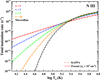 |
Fig. A.2 Comparison of total EII rate coefficients for N III between our calculations and KAPPA database (Dzifčáková et al. 2021) at density of 107 cm−3. Lines of different colors represent different energy distributions. |
Taking N II and N III as examples, we compared the total EII rate coefficients we calculated with those in the KAPPA database (Dzifčáková et al. 2021), which are presented in Figs. A.1 and A.2, respectively. It should be noted that the latest version of the KAPPA database is based on the widely used CHIANTI 10 database Dzifčáková et al. (2021). Furthermore, the ionization rate coefficients in the KAPPA database do not include density information, so we compare our results calculated at a density of 107 cm−3 with those from KAPPA. The comparison results indicate that, for N II, our calculations agree better with the KAPPA database for the kappa distributions. For the Maxwellian distribution, our calculated rate coefficients are slightly higher the KAPPA values. Moreover, for the N III ion, although our calculations are likewise marginally higher than KAPPA under both kappa and Maxwellian distributions, overall the two datasets are in good agreement, which validates the accuracy of our calculations for EII rate coefficients.
 |
Fig. A.3 Comparison of RR rate coefficients between our calculations and FLYCHK (Chung et al. 2005) as well as ADAS(Summers & O’Mullane 2011) of N II to N VII. |
Similarly, we also compared the recombination rate coefficients for N ions with the ADAS database (Summers & O’Mullane 2011) and the FLYCHK code (Chung et al. 2005). The comparison of RR rate coefficients for all N ions is presented in Fig. A.3. For N II, our calculations agree well with FLYCHK at higher temperatures and are slightly higher than those in ADAS expect for a temperature of 104 K. For N III, overall, our calculations are slightly higher than those of FLYCHK and ADAS. In terms of N IV, our RR rate coefficients are slightly higher than FLYCHK and ADAS at low temperature. For N V, the present values coincide exactly with ADAS, whereas for N VI and N VII they are in good agreement with both ADAS and FLYCHK, confirming the reliability of our computations.
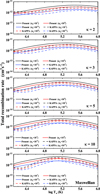 |
Fig. A.4 Comparison of total recombination rate coefficients between our calculations and KAPPA(Dzifčáková et al. 2021) of N II. The solid lines represent our calculated results, and the dashed lines represent the KAPPA results. Different colors correspond to different densities. |
Additionally, taking N II and N III as examples, we also compared our total recombination rate coefficients with those of the KAPPA database (Dzifčáková et al. 2021), as shown in Figs. A.4 and A.5, respectively. Unlike ionization, the KAPPA database provides total recombination rate coefficients at various densities. Therefore, we compared our recombination rate coefficients calculated at three electron densities, i.e., 107 cm−3, 109 cm−3 and 1011 cm−3, with the corresponding KAPPA results. It can be observed that for N II our calculations are slightly higher than those in KAPPA, whereas for N III the opposite is true. Nevertheless, overall our calculations agree well with the KAPPA database.
 |
Fig. A.5 Comparison of total recombination rate coefficients between our calculations and KAPPA(Dzifčáková et al. 2021) of N III. The solid lines represent our calculated results, and the dashed lines represent the KAPPA results. Different colors correspond to different densities. |
Appendix B Density suppression factor
In this section, we take N II as an example and present our calculated density SF in Fig. B.1. These results indicate that the density suppression effect is more prominent for the κ distribution than for the Maxwellian. For κ = 2, at a specific temperature, the suppression is approximately 6.5% higher than that observed in the Maxwellian case. The effect is strongest at lower temperatures and decreases as temperature increases. Additionally, higher electron densities lead to stronger suppression.
 |
Fig. B.1 Density SF of N II ion at Ne = 107 cm−3 (left) and Ne = 1011 cm−3 (right), plotted as a function of temperature. Lines of different colors represent different energy distributions. |
All Tables
Ground and excited states included in the calculations of excitation and deexcitation rate coefficients.
All Figures
|
Fig. 1 Comparison of the Maxwellian distribution and κ distributions at a temperature of 1.16 × 10⁵ K. Different colors represent the different energy distributions. |
| In the text | |
|
Fig. 2 Level populations of N I, N II, N III, and N IV as a function of electron density. The numbers 00, 01, 02, etc., refer to the energy levels listed in Table 2. Different colors represent different electron energy distributions. |
| In the text | |
|
Fig. 3 Level populations of N I, N II, N III, and N IV as a function of temperature. The numbers 00, 01, 02, etc., refer to the energy levels listed in Table 2. The selected electron density is 1011 cm−3. Different colors indicate different electron energy distributions. |
| In the text | |
|
Fig. 4 Spectrum of N III, with the transition from 2s12p2 to 2s22p1. Different colors correspond to different densities. |
| In the text | |
|
Fig. 5 Dependence of the spectral intensity ratio of N III on electron density. The double-dot-dashed line represents the ratio of the transition intensity from 2s12p2 4P1/2 to 2s22p1 2P3/2 to that from 2s12p2 4P5/2 to 2s22p1 2P3/2 (R1). The dashed line represents the ratio of the transition intensity from 2s12p2 4P3/2 to 2s22p1 2P3/2 to that from 2s12p2 4P5/2 to 2s22p1 2P3/2 (R2). Different colors correspond to different energy distributions. |
| In the text | |
|
Fig. 6 Dependence of the spectral intensity ratio of N III on electron temperature. The meanings of the different lines are the same as in Fig. 5. |
| In the text | |
|
Fig. 7 DI and EA rate coefficients of N I and N II. Different colors correspond to different energy distributions, and the different line shapes represent different electron densities. |
| In the text | |
|
Fig. 8 DI and EA rate coefficients of N III and N IV. Different colors correspond to different energy distributions, and the different line shapes represent different electron densities. |
| In the text | |
|
Fig. 9 DI and EA rate coefficients of N V, as well as the EA rate coefficients of N VI and N VII. Different colors correspond to different energy distributions, and the different line shapes represent different electron densities. |
| In the text | |
|
Fig. 10 PI rate of nitrogen. Different colors correspond to different ions, and the different line shapes represent different electron densities. |
| In the text | |
|
Fig. 11 DR rate coefficients of N I. Different colors correspond to different energy distributions, and the different line shapes represent different electron densities. |
| In the text | |
|
Fig. 12 DR and RR rate coefficients of N II to N VII. Different colors correspond to different energy distributions, and the different line shapes represent different electron densities. |
| In the text | |
|
Fig. 13 Total recombination rate coefficients of N II to N VII. Different colors correspond to different energy distributions, and the different line shapes represent different electron densities. |
| In the text | |
|
Fig. 14 Ionization equilibrium of N at three different electron densities, including the effects of EII, RR, and DR processes without density suppression. Different colors correspond to different charge states, and the different line shapes represent different electron densities. |
| In the text | |
|
Fig. 15 Ionization equilibrium of N, incorporating the influence of density suppression at a density of 1011 cm−3. Different colors correspond to different charge states. The solid lines denote the ionization equilibrium obtained with the density suppression effect included, whereas the dashed lines show the results without this suppression effect. |
| In the text | |
|
Fig. 16 Influence of the PI process on the ionization equilibrium of nitrogen. Different colors correspond to different charge states, and the selected density is 1011 cm−3. The solid lines represent calculations that include the PI process, and the dashed lines correspond to those without it. |
| In the text | |
|
Fig. 17 Final ionization equilibrium of nitrogen including all atomic processes, namely EII, PI, RR, and suppressed DR. Different colors correspond to different charge states, and the different line shapes represent different electron densities. |
| In the text | |
|
Fig. 18 Comparison of the ionization equilibrium for N from our calculations and KAPPA (Dzifčáková et al. 2021) at a density of 107 cm−3. Different colors correspond to different charge states. |
| In the text | |
|
Fig. A.1 Comparison of total EII rate coefficients for N II between our calculations and KAPPA database (Dzifčáková et al. 2021) at density of 107 cm−3. Lines of different colors represent different energy distributions. |
| In the text | |
|
Fig. A.2 Comparison of total EII rate coefficients for N III between our calculations and KAPPA database (Dzifčáková et al. 2021) at density of 107 cm−3. Lines of different colors represent different energy distributions. |
| In the text | |
|
Fig. A.3 Comparison of RR rate coefficients between our calculations and FLYCHK (Chung et al. 2005) as well as ADAS(Summers & O’Mullane 2011) of N II to N VII. |
| In the text | |
|
Fig. A.4 Comparison of total recombination rate coefficients between our calculations and KAPPA(Dzifčáková et al. 2021) of N II. The solid lines represent our calculated results, and the dashed lines represent the KAPPA results. Different colors correspond to different densities. |
| In the text | |
|
Fig. A.5 Comparison of total recombination rate coefficients between our calculations and KAPPA(Dzifčáková et al. 2021) of N III. The solid lines represent our calculated results, and the dashed lines represent the KAPPA results. Different colors correspond to different densities. |
| In the text | |
|
Fig. B.1 Density SF of N II ion at Ne = 107 cm−3 (left) and Ne = 1011 cm−3 (right), plotted as a function of temperature. Lines of different colors represent different energy distributions. |
| In the text | |
Current usage metrics show cumulative count of Article Views (full-text article views including HTML views, PDF and ePub downloads, according to the available data) and Abstracts Views on Vision4Press platform.
Data correspond to usage on the plateform after 2015. The current usage metrics is available 48-96 hours after online publication and is updated daily on week days.
Initial download of the metrics may take a while.