| Issue |
A&A
Volume 708, April 2026
|
|
|---|---|---|
| Article Number | A203 | |
| Number of page(s) | 14 | |
| Section | Extragalactic astronomy | |
| DOI | https://doi.org/10.1051/0004-6361/202556032 | |
| Published online | 08 April 2026 | |
Novel z ∼ 10 auroral line measurements extend the gradual offset of the fundamental metallicity relation deep into the first gigayear of cosmic time
1
Cosmic Dawn Center (DAWN), Denmark
2
Niels Bohr Institute, University of Copenhagen, Jagtvej 128, 2200 Copenhagen N, Denmark
3
Department of Astronomy, University of Geneva, Chemin Pegasi 51, 1290 Versoix, Switzerland
4
Department of Physics & Astronomy, University College London, London WC1E 6BT, UK
5
Institute for Astronomy, University of Edinburgh, Royal Observatory, Edinburgh EH9 3HJ, UK
6
Leiden Observatory, Leiden University, P.O. Box 9513, NL-2300 RA, Leiden, The Netherlands
7
DTU Space, Technical University of Denmark, Elektrovej 327, DK2800 Kgs. Lyngby, Denmark
8
Institute of Science and Technology Austria (ISTA), Am Campus 1, 3400 Klosterneuburg, Austria
★ Corresponding author.
Received:
19
June
2025
Accepted:
30
January
2026
Abstract
The mass assembly and chemical enrichment of the first galaxies provide key insights into their star formation histories and the earliest stellar populations at cosmic dawn. Here we compile and utilise new, high-quality spectroscopic JWST/NIRSpec Prism observations from the JWST archive. In particular, we extend the wavelength coverage beyond the standard pipeline cut-off (5.3 μm) up to 5.5 μm, which enables for the first time a detailed examination of the rest-frame optical emission-line properties for galaxies at z ≈ 10. Crucially, the improved calibration allows us to detect Hβ and the [O III] λλ4959, 5007 doublet and resolve the auroral [O III] λ4363 line for the 11 galaxies in our sample (z = 9.3 − 10.0) to obtain direct Te-based metallicity measurements. We find that the interstellar medium (ISM) of all galaxies shows high ionisation fields and electron temperatures, with derived metallicities in the range 12 + log(O/H) = 7.1 − 8.3 (3–50% solar), consistent with previous strong-line diagnostics based on JWST data at high redshifts. We derive an empirical relation for MUV and 12 + log(O/H) at z ≈ 10, useful for future higher-redshift studies, and show that the sample galaxies are ‘typical’ star-forming galaxies though with relatively high specific star formation rates (median sSFR = SFRHβ/M★ = 38 Gyr−1) and with evidence of bursty star formation on 10 Myr versus 100 Myr timescales (log10(SFR10/SFR100)≈0.7). Combining the rest-frame optical line analysis and detailed UV to optical spectro-photometric modelling, we determine the mass-metallicity relation (MZR) and the fundamental metallicity relation (FMR) of the sample, pushing the previous redshift frontier of these measurements to z = 10. These results, together with literature measurements, point to a gradually decreasing MZR at higher redshifts, with a break in the FMR at z ≈ 3, decreasing to metallicities ≈3× lower at z = 10 than observed in galaxies during the majority of cosmic time at z = 0 − 3, likely caused by massive pristine gas inflows diluting the observed metal abundances during early galaxy assembly at cosmic dawn.
Key words: galaxies: evolution / galaxies: formation / galaxies: high-redshift
© The Authors 2026
 Open Access article, published by EDP Sciences, under the terms of the Creative Commons Attribution License (https://creativecommons.org/licenses/by/4.0), which permits unrestricted use, distribution, and reproduction in any medium, provided the original work is properly cited.
This article is published in open access under the Subscribe to Open model. This email address is being protected from spambots. You need JavaScript enabled to view it. to support open access publication.
1. Introduction
Probing the chemical enrichment of the first galaxies in the early Universe is key to constraining the physical processes that regulate their formation and evolution via gas inflows and outflows, star formation, and the synthesis of heavier elements in stellar cores. This process has been characterised by the scaling relation between the stellar mass and chemical abundance of oxygen, known as the mass-metallicity relation (MZR; Lequeux et al. 1979; Tremonti et al. 2004; Lee et al. 2006; Erb et al. 2006; Kewley & Ellison 2008). Perhaps more fundamental is the additional scaling with the star formation rate (SFR), called the fundamental metallicity relation (FMR; Ellison et al. 2008; Mannucci et al. 2010; Lilly et al. 2013; Andrews & Martini 2013; Curti et al. 2020), which has been found to be constant out to z ≈ 3 (Sanders et al. 2021), throughout the majority of cosmic time. This implies an equilibrium between gas accretion, star formation, and metal enrichment, potentially representing the universal scaling between the molecular gas mass surface density and star formation (Baker et al. 2023).
Rest-frame optical spectroscopy of strong nebular emission lines enables key insights into the physical properties and chemical enrichment of star-forming regions in galaxies through cosmic time (see e.g. Maiolino & Mannucci 2019; Kewley et al. 2019, for reviews). With the advent of JWST and its suite of sensitive, near-infrared spectroscopic capabilities (Jakobsen et al. 2022), it is now possible to measure and constrain rest-frame optical nebular emission lines out to very high redshifts. The first studies of a statistical sample of galaxies at z ≈ 8 with detected rest-frame optical emission lines (Langeroodi et al. 2023; Heintz et al. 2023a; Sanders et al. 2024) revealed a significantly decreasing metallicity at a given stellar mass compared to past measurements out to z ≈ 3. This was later confirmed by larger JWST samples (Nakajima et al. 2023; Curti et al. 2024; Morishita et al. 2024), and for very low-stellar-mass (M★ ∼ 106 M⊙; Chemerynska et al. 2024) to near-solar metallicities (Rowland et al. 2026). Perhaps most surprising was the apparent offset from the FMR towards 0.5 dex lower metallicities for a given stellar mass and SFR (Heintz et al. 2023a), hinting at a transition period for high-redshift galaxies dominated by pristine gas inflows, though the exact redshift is still debated (constrained to within z ∼ 4 − 8; Nakajima et al. 2023; Curti et al. 2024). Strong-line measurements further enable the determination of the relative elemental abundances and the ionisation fields of the interstellar medium (ISM; e.g. Schaerer et al. 2022; Arellano-Córdova et al. 2022, 2025; Heintz et al. 2023b; Trump et al. 2023; Shapley et al. 2023a) for some of the most distant galaxies known out to z ≈ 9.
Most of the previous metallicity measurements of high-redshift galaxies have relied on strong-line diagnostics due to the inaccessibility of the temperature-sensitive [O III] λ4363 auroral lines, either due to their intrinsic faintness or because they are blended with Hγ in low-resolution spectra. However, a growing number of direct measurements using the direct ‘Te-method’ are now being reported based on JWST grating spectra (Laseter et al. 2024; Sanders et al. 2024; Scholte et al. 2025; Cullen et al. 2025; Sanders et al. 2025), which has been crucial to calibrate the empirical strong-line relations for the majority of galaxies with no auroral line detection.
Despite the growing number of Te-based 12 + log(O/H) estimates, there are still relatively few at z > 9. Here we utilise new, custom reductions of recent JWST/NIRSpec Prism spectroscopic data, expanding the wavelength coverage out to 5.5 μm (up from 5.3 μm), to investigate the rest-frame UV and optical lines up to and including the [O III] λλ4959, 5007 line doublet at z = 10.0. These we use to benchmark against existing high-redshift strong-line diagnostics and determine fundamental galaxy scaling relations up to the highest redshifts achievable by JWST/NIRSpec.
We structure the paper as follows. In Sect. 2 we present our new spectroscopic reductions of archival JWST data and detail the sample compilation. In Sect. 3 we describe the emission-line analyses and spectro-photometric modelling and in Sect. 4 we present the new empirical galaxy scaling relations at z ≈ 10. In Sects. 5 and 6 we discuss and conclude on our work. Throughout the paper we assume the standard concordance cosmology, with a flat, Λ-cold-dark-matter-dominated Universe. We adopt the cosmological parameters from Planck Collaboration VI (2020) and the solar abundances from Asplund et al. (2009) with 12 + log(O/H)⊙ = 8.69.
2. Observations
For this work, we compiled and utilised the archival JWST data reduced and processed as part of the DAWN JWST Archive (DJA; Brammer & Valentino 2025)1. This online repository contains reduced images, photometric catalogues, and spectroscopic data for public JWST data products. The raw spectroscopic data are retrieved from MAST, before they are processed with MSAExp (Brammer 2023)2, as detailed in Heintz et al. (2025, for version 2, v2) and de Graaff et al. (2025, for v3), respectively.
Here we present and utilise the most recent spectra from v4 of the DJA spectroscopic archive (see also Valentino et al. 2025). We focus on the spectra observed with the JWST/NIRSpec Prism configuration (Jakobsen et al. 2022), which nominally covers λ = 0.6 − 5.3 μm with a resolving power of ℛ ≈ 100. Briefly, DJA-v4 uses updated JWST reference files, and includes a bar shadow correction, overall improving the absolute and colour-dependent flux calibration. For the first time, we extend the wavelengthrange reference file3 to include the second- and third-order Prism spectra, which were cut from the JWST pipeline to avoid the higher-order contamination on the primary first spectral order (Jakobsen et al. 2022). These, however, appear at predictable locations and intensities, and are therefore now carefully calibrated into the DJA-v4 reductions to include the full response of the telescope and thereby recover the full spectrum recorded on the detector (see also Valentino et al. 2025, for details on the same procedure on the higher-resolution grating spectra). This effectively extends the wavelength coverage of NIRSpec Prism to 5.5 μm. The final 1D spectra were optimally extracted (Horne 1986) and the flux calibrations are generally accurate to the photometry (see below). The v4 reductions have been run and processed on the entire DJA, including also more recent public JWST/NIRSpec observations, and can be found on the dedicated online repository4.
Consequently, we can now detect and constrain the rest-frame optical emission lines such as the crucial [O III] λλ4959, 5007 doublet up z = 10.0 with JWST/NIRSpec (instead of only up to z ≈ 9.5 with standard pipeline products). Due to increasing spectral resolution with wavelength, and the generally higher delivered resolving power relative to predicted resolution (see also de Graaff et al. 2024), we measure up to ℛ ≈ 500 at 5.5 μm. This increased resolution is sufficient to spectroscopically resolve the [O III] λ4363 auroral line transition from Hγ at z ≳ 9.0, allowing direct, Te-based metallicity estimates at z = 9.0 − 10.0. We compiled a set of 11 galaxies from DJA-v4 with JWST/NIRSpec Prism spectra, by requiring a robust detection of Hβ (S/N > 5) and wavelength coverage of the [O III] λλ4959, 5007 doublet. This mainly includes galaxies observed as part of the major JWST spectroscopic surveys: CAPERS (prog. ID: 6368, PI: Dickinson; Kokorev et al. 2025), JADES (prog. IDs: 1181 and 3215, PI: Eisenstein; Bunker et al. 2024; Eisenstein et al. 2026, 2025), UNCOVER (prog. ID: 2561, PIs: Labbe and Bezanson; Bezanson et al. 2024), RUBIES (prog. ID: 4233, PIs: de Graaff & Brammer; de Graaff et al. 2025), and RXJ DDT (prog. ID: 2767, PI: Kelly). The final sample is summarised in Table 1.
Sample overview with derived redshifts and rest-frame optical emission-line fluxes, or 3σ upper limits.
For each galaxy, the photometric data obtained primarily with JWST/NIRCam through DJA (Valentino et al. 2023) were inspected, in order to photometrically calibrate the flux density of the spectra. Of the 11 galaxies in the sample, only two require a positive (> 1) scaling, consistent with slit loss. For these objects the spectra were calibrated using BAGPIPES during the spectro-photometric modelling of the spectral energy distribution (SED), and the calibrated spectra were used for line fitting. For the remainder of the sample, the photometry is either consistent with spectroscopy; not requiring rescaling, or lower than the spectrum for no obvious physical reason from inspecting the morphology. The analysis for these galaxies was carried out directly on the DJA-reduced spectra.
3. Analysis and results
3.1. Emission-line modelling
We modelled the most prominent rest-frame optical nebular emission lines detected in the spectra, from the (unresolved) [O II] λλ3726, 3729 doublet to the [O III] λλ4959, 5007 doublet line transitions. Due to the expanded wavelength coverage, the latter can now be measured up to z = 10.0, while simultaneously resolving the auroral [O III] λ4363 line from Hγ. We determined the line fluxes or upper bounds on the emission lines by modelling the full set of lines jointly with Gaussian line profiles (at vacuum wavelengths), tying the redshift and intrinsic width (convolved with the Prism spectral resolution). We modelled the underlying continuum with a simple first-order polynomial. To estimate the model parameters, we use dynamic nested sampling from DYNESTY (Speagle 2020), which allows for more complex distributions to be modelled (Koposov et al. 2022; Higson et al. 2019).
An example of the line fitting, highlighting the spectroscopically resolved [O III] λ4363 line, is shown in Fig. 1. We chose a 3σ detection limit for the [O III] λ4363 line, as we know the line-spread function, expected wavelength, and redshift of each galaxy precisely. Increasing the threshold to 5σ changes the derived limits on metallicity by ∼0.1 dex in each case, which has a minimal impact on the results of the paper. We note that 5σ flux limits result in extreme O3Hg and O33 line ratios, inconsistent with the detections, implying a 5σ cut may overestimate the line flux. We show zoom-ins of the Hγ-[O III] λ4363 region for all galaxies of the sample in Fig. 2, along with the signal-to-noise detection for each [O III] λ4363 line.
 |
Fig. 1. JWST/NIRSpec Prism 1D spectroscopy of the sample, shown in shades of blue, with the associated error spectrum as a shaded region. The positions of the main line transitions are highlighted by grey lines. The inset zooms in on the spectroscopically resolved Hγ + [O III] λ4363 emission lines, with the best-fit continuum and emission-line model for each galaxy shown by the pink lines. |
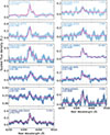 |
Fig. 2. Hγ and [O III] λ4363 regions for each galaxy are shown in shades of blue, along with the best fit emission line model in pink. The significance of the [O III] λ4363 line detection is shown in the top right corner of each subplot. |
We find that the observed spectral resolution is typically 1.20–1.70 higher than the nominal JWST/NIRSpec Prism curve at any given wavelength (see also e.g. de Graaff et al. 2024). The derived line fluxes and derived redshifts are summarised in Table 1.
The observed line fluxes were corrected for dust-reddening using SED-derived extinction AV values (multiplied by a factor of η = 2 to account for the difference between stellar and nebular AV), from the BAGPIPES fits outlined in Sect. 3.3. Emission line fluxes were corrected with the average nebular attenuation curve from Reddy et al. (2026), derived for high-z galaxies with Balmer and Paschen decrements.
Of course, the galaxy-to-galaxy variation in the dust curve is large (Salim & Narayanan 2020), and JWST studies at high-z have suggested that the dust curve at fixed AV is flattening with increasing redshift (Shivaei et al. 2025; Markov et al. 2025a,b). We find the sample to be generally dust-poor, with a maximum AV = 0.36, and mean AV ∼ 0.2. The dust-corrected line fluxes are used for emission line ratios, as well as for derivations of Te, 12 + log(O/H), and SFR(Hβ). When assuming other commonly used dust laws (e.g. Calzetti et al. (2000), Gordon et al. (2003) SMC, or Cardelli et al. (1989) Milky Way) the final metallicities and log(SFR) remain within reported uncertainties, with median changes of < 0.02 dex in each case, and maximum changes of ≲0.05 dex.
Figure 3 shows the main line ratios of the strongest nebular lines, highlighting the typical ionisation fields, electron temperatures, and diagnostics to separate active galactic nuclei (AGNs) from star-forming galaxies. Here we also compare to the low-redshift (z < 0.3) galaxy sample from the Sloan Digital Sky Survey (SDSS; Aihara et al. 2011), for reference. The SDSS line fluxes were corrected for dust attenuation using the Balmer decrement, assuming Hα/Hβ = 2.86 (Case B, Te = 10 000 K), and a Cardelli et al. (1989) dust curve.
 |
Fig. 3. Line flux ratios of the z = 9 sample, with [O III] λ4363 detections in hot pink, and 3σ upper limits in pale pink. The light blue points show z ≈ 0 galaxies with [O III] λ4363 detections from from SDSS-DR15, for comparison. The dark blue points represent SDSS objects that lie in the AGN region of the [N II]/Hα Kauffmann et al. (2003) BPT diagram. Dashed lines represent AGN diagnostics utilising the [O III] auroral line from Mazzolari et al. (2024), calibrated using local and high-z samples of SFGs and AGNs. |
Strong nebular line ratios have typically been used to distinguish the intrinsic emission from AGNs or star-forming regions. The classic Baldwin-Phillips-Terlevich (BPT) diagram (Baldwin et al. 1981) separating the dominant emission components is based on the [O III] λ5007/Hβ versus [N II] λ6584/Hα line ratios. However, this is obfuscated at high redshifts due to the general increased intensity of the ISM ionisation fields (Calabrò et al. 2024; Roberts-Borsani et al. 2024), and we are unable to measure [N II] λ6584/Hα with NIRSpec beyond z ≈ 8.3. Nevertheless, we highlight the SDSS galaxies that lie above the [N II]/Hα BPT demarcation of Kauffmann et al. (2003) in dark blue, noting that our z = 9 − 10 sample generally lie in different line ratio regions to both the low-z SFGs and low-z AGNs. New classification diagnostics have therefore been developed, focusing particularly on the O3Hg =log10([O III] λ4363/Hγ) line ratio (Mazzolari et al. 2024; Backhaus et al. 2025). In panels (a)–(b) of Fig. 3, we show the O3Hg line ratios compared to O32 =log10([O III] λ5007/[O II] λ3727) and O33 =log10([O III] λ5007/[O III] λ4363), representing the ionisation field and Te, respectively. We note that the O3Hg line ratios are only slightly higher than the low-redshift reference sample, likely due to a combination of higher Te but lower metallicities. While the majority of our sample are located in the star-forming locus for panels (a)–(b), they lie close to the boundary, and many are situated in the AGN region (albeit also along the boundary) for panel (c), where O3Hg is plotted with Ne3O2 =log10([Ne III] λ3869/[O II] λ3727). Given the difficulty of distinguishing star-forming galaxies and AGNs at high z, and relying on faint emission lines for the diagnostics, we cannot rule out the presence of AGNs in the sample. If present, the contribution could affect metallicity and stellar mass measurements. However, since the sample lies along the boundary, and there is no overwhelming evidence to suggest that AGNs are present, we assume that these are star-forming sources in the following analysis.
In Panel (d), we show O32 relative to O33, the latter inversely correlating to the electron temperature, Te, of the H II region. We find no clear correlation between the lines ratios for the galaxies at z = 9 − 10 but highlight the typically lower [O III] λ5007/[O III] λ4363 ratios at high z, indicating higher Te in the ISM of these galaxies. In Panel (e), we show the Ne3O2 line ratios versus the O32 ones, which are both sensitive to the same ionisation field, since [Ne III] and [O III] originate in the same high-ionisation zone of the H II region (with ionisation potentials greater than ∼40 and 35 eV). We find that both these line ratios are substantially higher than for the typical low-redshift galaxy population, as was also found previously for JWST-observed galaxies up to z ∼ 8 (Schaerer et al. 2022; Curti et al. 2023; Roberts-Borsani et al. 2024). This indicates a higher ionisation parameter in these early systems, with median log U ≈ −2, quantified from diagnostics based on O32 and Ne3O2 (Díaz et al. 2000; Witstok et al. 2021).
3.2. Direct Te-based metallicities
We determined the metallicities using the direct ‘Te-based’ method (Peimbert et al. 2017; Pérez-Montero 2017; Kewley et al. 2019; Osterbrock & Ferland 2006), which relies on measuring the electron temperature, Te, to determine gas-phase metallicity 12 + log(O/H). This assumes electron densities of ne ≲ 105 cm−3, below the critical densities of [O III] λ5007 and [O III] λ4363 (Osterbrock & Ferland 2006) that appear to be common for galaxies at z ∼ 10 (Hsiao et al. 2024a; Isobe et al. 2023; Topping et al. 2025).
We estimated the electron temperature, Te, with the [O III] λ4363/[O III] λ5007 ratio, using the getTemDen routine in PYNEB (Luridiana et al. 2015). As the [O II] doublet is unresolved we do not have a direct constrain on the electron density. However, ne = 300 cm−3 is typical of star-forming galaxies at z ∼ 2.3 (Sanders et al. 2016), although JWST results have shown that there is likely to be a trend of increasing electron density with redshift (Topping et al. 2025; Abdurro’uf et al. 2024; Li et al. 2025a; Isobe et al. 2023; Harikane et al. 2025). While we fiducially assume an electron density of ne = 300 cm−3, we find changing the density up to ne ∼ 1 × 104 cm−3 has at most a 0.02 dex impact on the abundance measurements. Harikane et al. (2025) have suggested that a more accurate method would be to combine JWST and ALMA observations and use a two-zone ISM model to trace both high and low-density regions, as assuming a constant density and temperature throughout the ISM may result in one underestimating the oxygen abundance by up to 0.8 dex.
As determining a singly ionised oxygen abundance, O+, requires a temperature that traces the low-ionisation zone of the gas, we assume a relation between temperatures of the high and low ionisation zones Te([O II]) = 0.7 × Te([O III]) + 3000 K from Campbell et al. (1986). Cataldi et al. (2025) suggest a new T3 − T2 relation for z ∼ 2 − 3, although using this calibration changes the oxygen abundance of the sample on average 0.01 dex, as the galaxies are highly ionised so the O+ abundance is generally low. The total oxygen abundance was then calculated by summing the contributions from different ionic abundances O/H+ = O+/H+ + O++/H+ obtained with getIonAbundance. The contribution from O+ + + was not included as it is likely to be negligible even under the most extreme ISM conditions (Cullen et al. 2025; Berg et al. 2021). The errors on all gas-phase properties were obtained using 1000 Monte Carlo simulations, whereby line fluxes were perturbed randomly according to their measured uncertainties. We employed the transition probabilities and collisional strengths included in PYNEB, and all of the atomic data from Froese Fischer & Tachiev (2004), collisional data from Kisielius et al. (2009) for O+, and Aggarwal & Keenan (1999) for O++.
The direct metallicities (and 3σ upper limits) for the full sample are listed in Table 2 and shown in Fig. 4, ranging from 12 + log(O/H) ≈7.1 − 8.3. We compare them to high-z literature diagnostics Laseter et al. (2024) and Scholte et al. (2025) in panel (a) as well as high-z from Sanders et al. (2024) and Sanders et al. (2025) and high equivalent width (EW) low-z diagnostics from Nakajima et al. (2022) in panels (b)–(f). Our sample is generally in good agreement with these calibrations (with considerable scatter, as was also seen in previous works), though we do not have a large enough statistical sample to distinguish between different calibrations that diverge. Our derived metallicities for RXJ2129-11767-11027 and JADES-GS-265801 are consistent within ∼0.1 dex with the values reported in previous literature: respectively, 12 + log(O/H) = 7.48 ± 0.08 (Williams et al. 2023, from strong-line ratios) and 7.49 ± 0.11 (Curti et al. 2025, using the direct method, with ionisation correction factors).
 |
Fig. 4. Te-based metallicities and strong-line ratios for the z > 9 sample. Direct oxygen abundances are represented by hot pink square markers, with 3σ upper limits in pale pink. We compare to various literature strong-line diagnostics: the solid and dashed blue relations show Laseter et al. (2024) and Scholte et al. (2025)
|

Main galaxy properties for our z > 9 sample, including UV magnitude, MUV, UV continuum slope, βUV, stellar mass, SFRs derived from Hβ, electron temperature, Te, and direct Te based metallicities derived using PYNEB.
3.3. Spectro-photometric SED modelling
To derive the stellar continuum properties of our sample, in particular the stellar masses, we performed spectro-photometric modelling of the SED of each source based on the JWST/NIRSpec PRISM spectroscopy and available broadband NIRCam photometry. We summarise our modelling methods below.
In order to estimate the SED model posteriors, we used the code Bayesian Analysis of Galaxies for Physical Inference and Parameter EStimation (BAGPIPES, Carnall et al. 2018, 2019), which performs nested-sampling using the NAUTILUS (Lange 2023) algorithm. Within BAGPIPES, we used the Binary Population and Spectral Synthesis code (BPASS) v2.2.15 stellar population synthesis (SPS) models (Stanway & Eldridge 2018) to build galaxy SEDs based on a broken power-law initial mass function (IMF), where the slope of the power law is α1 = −1.30 for M★ ∈ (0.1, 0.5) M⊙ and α2 = −2.35 for M★ ∈ (0.5, 300) M⊙. We used nebular line and continuum emission models from the CLOUDY photoionisation code (Ferland et al. 2017; Byler et al. 2017), whereby the CLOUDY grids were calculated using the BPASS SPS models as the input ionising source.
To account for slit losses, the JWST/NIRSpec PRISM spectra were flux-calibrated to the NIRCam broadband photometry self-consistently within the BAGPIPES framework with a second-order Chebyshev polynomial. Gaussian priors were set on the polynomial coefficients by performing an initial least-squares fit to the ratio between the observed photometry to the synthetic photometry (calculated by integrating the NIRSpec spectrum through the NIRcam filter profiles6). From an initial SED modelling run, we find that only two sources in our sample require photometric scaling: JADES-GN-3990 and UNCOVER-2561-3686 (using F090W, F115W, F356W, and F444W and F115W, F150W, F200W, F277W, F356W, and F444W, respectively). For the rest, we performed SED modelling without the calibration described above.
We modelled the SEDs with a non-parametric continuity star formation history (SFH; Leja et al. 2019), which allows for flexible SFRs in a sequence of user-defined time steps. The initial few time step edges were fixed in look-back time at [0, 10, 50, 100] Myr, after which the timesteps were equally spaced in logarithmic look-back time between 100 Myr and the age of the Universe at z = 30. The number of time steps therefore is redshift-dependent. We imposed a Student’s t distribution on the change in the SFR between adjacent time bins, with the distribution being centred at 0 with a scale factor σ = 0.3 and ν = 2 (Leja et al. 2019). We set a logarithmic prior on the formed stellar mass, Mformed/M⊙ ∈ (106, 1014). We set a Gaussian prior on the metallicity, centred on the direct Te-based measurements derived in Sect. 3.2 with a scatter of 10% Z⊙. For galaxies with only a lower limit on Te-based metallicities, strong-line diagnostics were instead used to quantify the oxygen abundance (see Eq. (2); Sect. 4.3).
The dust was modelled with a Salim et al. (2018) dust curve, whereby we fixed the slope of the attenuation curve to δ = −0.3 and the strength of the 2175 Å UV bump was fitted in the range B ∈ (0, 3) with a uniform prior. An extra factor of attenuation was applied to starlight within stellar birth clouds, where η = 2. We adopted a uniform prior on the V-band attenuation, where AV ∈ (0, 1) mag.
The nebular ionisation parameter was varied in the range log U ∈ ( − 4, −1) with a uniform prior. We set a tight Gaussian prior on the redshift centred at the spectroscopic redshift derived from MSAEXP on the DJA, with σz = 0.001 × (1 + zspec). The velocity dispersion was fixed to 100 km/s. A logarithmic prior was set on the white noise scaling in the range (1.,10.). We caution that the posterior parameter estimates from the SED modelling are heavily model-dependent, where in particular the stellar mass may be subject to ‘outshining effects’ (e.g. Giménez-Arteaga et al. 2023; Narayanan et al. 2024), and the assumed SFH and IMF (e.g. Carnall et al. 2018; Leja et al. 2019; Steinhardt et al. 2023; Strait et al. 2023).
4. Galaxy properties at z ≈ 10
4.1. Rest-frame UV properties
The derived galaxy properties are summarised in Table 2. We first consider the direct, measured properties of the targeted galaxies at z = 9 − 10.
For the absolute rest-frame UV magnitude, we integrated the flux density of the spectrum with a 100 Å top-hat filter centred at rest-frame 1500 Å. We fitted a standard power-law slope, assuming Fλ, obs ∝ λ−βUV to determine βUV, carefully masking the most prominent nebular emission lines in the modelling. The large scatter, from βUV = −1.5 to −2.8 and MUV = −16 to −21 mag, is consistent with larger samples using photometric (Topping et al. 2024; Cullen et al. 2024; Austin et al. 2025) and spectroscopic (Saxena et al. 2024; Dottorini et al. 2025; Tang et al. 2025) measurements. We do not observe any strong correlations between MUV and βUV in our spectroscopic sample at z = 9 − 10, where typically brighter, more massive galaxies would be expected to show redder rest-frame UV slopes.
In Fig. 5 we compare MUV to the oxygen abundance 12 + log(O/H). For comparison to our sample we plot Te-derived metallicities for the lensed galaxy MACS0647-JD1 at z = 10.17 (Hsiao et al. 2024a), and GN-z11 (Álvarez-Márquez et al. 2025) at z = 10.6. These studies make use of the MIRI Medium Resolution Spectrograph to measure [O III] λ5007 for z > 10. We also measure strong-line metallicities (see Sect. 4.3 for method) for the galaxies with only lower limits in 12 + log(O/H), and measure a best-fit relation of
 (1)
(1)
 |
Fig. 5. Direct Te-based metallicity 12 + log(O/H) versus (dust-corrected) UV magnitude, MUV. Also shown are the direct metallicity measurements of MACS0647-JD1 at z = 10.17 from Hsiao et al. (2024a) and GN-z11 at 10.6 from Álvarez-Márquez et al. (2025). We fitted an empirical relation to the measurements (including strong-line derived values where only Te-based lower limits are available), shown in solid black with 1σ errors represented by the shaded grey region. The best-fit relation is reported in the bottom right, with the associated Spearman and Pearson correlation coefficients, ρ and r, indicating a strong correlation; the most massive, UV-bright galaxies are more metal-enriched. |
The relationship observed is expected given that the most massive, star-forming galaxies are likely to also show higher metal enrichment at a given SFR. This strong correlation (with a Spearman coefficient ρ = −0.90 and Pearson coefficient r = −0.84) further provides a viable relation to infer the gas-phase metallicities for galaxies at z ≳ 10 with only measures of MUV.
Of the strong-line derived metallicities, 3/5 of the objects have lower values than the ‘lower-limit’ of the Te-method. Our strong-line method takes each available diagnostic into account, but the derived value can change substantially depending on the choice of ratios, i.e. UNCOVER-2561-3686 (also referred to as Gz9p3 in literature) has a Te-derived lower limit of 12 + log(O/H) > 8.38, with reports from Nakane et al. (2025) using the R2 diagnostic giving  , and Boyett et al. (2024b) from the Ne3O2 diagnostic 12 + log(O/H) = 7.6 ± 0.5. UNCOVER-2561-3686 and RUBIES-UDS-833482 have high R3 and R23 ratios that lie above the associated diagnostics. As was discussed before, we cannot rule out the presence of AGNs in the sample, which could boost line ratios and therefore affect metallicity derivations.
We do not recover any apparent trend relating βUV to 12 + log(O/H), whereby increased dust reddening would be expected to scale with the metallicity. The galaxies typically have bluer UV slopes and lower metallicities than the z ∼ 2 galaxies studied in Reddy et al. (2010), and are also less enriched than the local starburst galaxies that form the βUV − 12 + log(O/H) relation in Heckman et al. (1998). The lack of trend indicates that the rest-frame UV slope is likely not representing the overall dust content of high-redshift galaxies, potentially due to more dominating nebular continua at low metallicities (Cameron et al. 2024; Katz et al. 2025), although the nebular contribution derived from the EW of Hβ (Miranda et al. 2025) is in general fairly small (of the order of a few percent).
4.2. Star formation rates and timescales
The relationship between the SFR and stellar mass, M★, also known as the star-forming galaxy main sequence (SFMS), is tightly connected for star-forming galaxies, though varying in normalisation across redshifts (e.g. Brinchmann et al. 2004; Daddi et al. 2007; Whitaker et al. 2012; Speagle et al. 2014; Lee et al. 2015; Thorne et al. 2021). This indicates an evolving specific SFR (sSFR = SFR/M★), with galaxies at higher redshifts more actively forming stars at a given stellar mass (e.g. Topping et al. 2022). To investigate this relation at z ≈ 10, we here adopt M★ inferred from the non-parametric SFH model outlined in Sect. 3.3 and derive the SFR based on the dust-corrected Hβ Balmer line luminosity. This uniquely traces the ongoing star formation on relatively short, ∼10 Myr timescales, compared to standard UV- or SED-based estimates that trace SFRs over ∼100 Myr. We used the prescription from Shapley et al. (2023b) to determine SFRHβ based on Hα, assuming a constant ratio of Hα/Hβ = 2.76 dictated from the Case B recombination scenario at Te = 2 × 10⁴ K (Osterbrock & Ferland 2006) and the average metallicity for our sample of ≈10% solar.
In Fig. 6 we show the SFRHβ-M★ relation for the galaxies at z = 9 − 10, compared to the full JWST-PRIMAL sample at z = 3 − 9 (Heintz et al. 2025) and other recent literature measurements at z ≳ 7 (Heintz et al. 2023a). While the sample clearly show elevated SFRs at a given mass compared to more local estimates for galaxies at z = 0 − 4 (Thorne et al. 2021, SED-derived SFRs), and z = 4 − 7 (Clarke et al. 2024, Hα-derived SFRs), the SFMS is overall consistent in normalisation and slope with the other literature measurements at z ≳ 6, potentially with a mild increase in the SFR of 0.15 dex on average. This indicates only a marginal evolution in the SFMS from ≈1 Gyr to 500 Myr, consistent with the overall observed trend with redshift. The median sSFR is 38 Gyr−1, 2 − 5× the average value found for massive, UV bright galaxies at z = 6 − 8 (Topping et al. 2022). These results suggest that SFMS is already in place at z ≈ 10, just 470 Myr after the Big Bang, and that our sample is generally comprised of ‘typical’ but very active star-forming galaxies during this epoch.
 |
Fig. 6. Star-forming galaxy SFR − M★ main-sequence. The z > 9 galaxies are plotted in pink, with the weighted mean of the sample represented by the purple star. To compare, we plot the PRIMAL sample at z = 3 − 10 as grey points, with the median of stellar mass bins indicated by grey markers. The solid black error bars on these markers represent the error on the median, with grey error bars showing the standard deviation of the bin. We also plot the linear relation (and empirical scatter) of the best-fit SFMS for z = 7 − 10 from Heintz et al. (2023a) in light blue, with dark blue curves showing the evolution of the best-fit main sequence for z ∼ 0 − 4 from Thorne et al. (2021) and z ∼ 4 − 7 from Clarke et al. (2024). |
We now investigate the SFR timescales for the sample galaxies at z ≈ 10, searching for potential signs of short-lived bursts of star formation, which might be related to the observed overabundance of UV bright galaxies at z ≳ 10 (e.g. Sun et al. 2023; Gelli et al. 2024). We compare the SFRs derived from Hβ as a proxy for SFR10 and the SED-derived SFR on a 100 Myr timescale for the full galaxy sample at z = 9 − 10. We find that, on average, the SFR on 10 Myr to 100 Myr timescale is log10(SFR10/SFR100) = 0.7, which is ≳3× higher than the average value found at z ≈ 6 (Endsley et al. 2025; Cole et al. 2025), but consistent with individual galaxy studies at z ≳ 10 (Kokorev et al. 2025). These measurements thus provide strong evidence of highly stochastic or more bursty star formation in the general population of star-forming galaxies at z ≳ 10.
4.3. Mass-metallicity relation at z ≈ 10
We then consider the MZR for our sample in Fig. 7, extending previous analyses with JWST out to z > 9. The scaling relation between stellar mass and gas-phase metallicity is among the most studied galaxy relationships, with a relatively small intrinsic scatter (∼0.1 dex) and a strong correlation, showing that more massive systems become more metal-enriched. The shape of the local MZR shows a steeper slope at low masses, which flattens at higher masses, with a turnover of ∼ 1010 M⊙ (see e.g. Maiolino & Mannucci 2019, for a review). Previously, detections of [O III] λ4363 at z > 3 were mostly inaccessible, but thanks to the sensitivity and wavelength coverage of NIRSpec, and the increased sample size of direct metallicity measurements, early JWST studies of the MZR suggest the relationship is already in place at z = 6 − 8 (e.g. Morishita et al. 2024). We compared our direct Te-based measurements and lower limits in metallicity to various high-z MZR relations from literature, which use both the direct Te method (Morishita et al. 2024; Chakraborty et al. 2025) and strong-line calibrations (Heintz et al. 2023a; Nakajima et al. 2023; Curti et al. 2024; Chemerynska et al. 2024; Sarkar et al. 2025). As was expected, our sample galaxies are similarly less enriched for a given stellar mass than local galaxies (e.g. Curti et al. 2020), between ∼0.5 − 1.0 dex.
 |
Fig. 7. Mass-metallicity relation at z > 9. Direct Te metallicities and lower limits for the z > 9 sample are shown in hot pink and light pink, respectively, with the weighted mean and 1σ error of the sample indicated by the purple star. Various MZRs from literature are plotted (Heintz et al. 2023a; Curti et al. 2020; Morishita et al. 2024; Nakajima et al. 2023; Curti et al. 2024; Chemerynska et al. 2024; Chakraborty et al. 2025). Light grey scatter points represent the PRIMAL z = 3 − 10 sample, with circular grey markers and their associated solid black error bars being the median and 1σ error of stellar mass bins. The grey error bars represent the standard deviation of mass bins. The bold solid black line shows the best fit to the PRIMAL stellar-mass bins. |
As a benchmark, we also included additional high-z galaxies from the JWST-PRIMAL archival study (Heintz et al. 2025, grey markers and scatter points), selected at z > 3 and with Hβ detections with S/N > 3. The metallicities of these galaxies were obtained using strong-line calibrations from Sanders et al. (2024) and Laseter et al. (2024), using a joint χ2 approach taking into account each strong-line ratio available ( , Ne3O2, R3, R2, R23, and O32), inversely weighted by its intrinsic scatter.
 (2)
(2)
where x = 12 + log(O/H), Robs is the observed line ratio with error σobs, Rcal is the modelled line ratio, and σcal is the reported scatter of the diagnostic (Curti et al. 2020).
We divided 735 galaxies into seven stellar-mass bins of 105 galaxies each, and fitted a simple log-linear relation to the bins (solid black line), with a best-fit relation of 12+ log(O/H) = (0.42 ± 0.04) log10(M★) + (4.19 ± 0.34). The weighted mean of our Te-based sample (depicted by a purple star) lies in line with the derived relation for the PRIMAL galaxies. Using the updated calibrations from Sanders et al. (2025), metallicity values of the stellar-mass bins remain consistent within the error bars (median change 0.02 dex).
4.4. Deviation from the fundamental metallicity relation
The MZR has been observed to have an additional dependence on the SFR, with highly star-forming galaxies appearing to be more metal-poor at a given stellar mass. To reduce the scatter on the MZR, Mannucci et al. (2010) introduced the FMR with an additional parametrisation for SFR:
 (3)
(3)
where α is a constant between 0 and 1, chosen to minimise the scatter in μα − Z space (Mannucci et al. 2010; Andrews & Martini 2013). The FMR appears universally constant out to z ≈ 3 (Sanders et al. 2021), though recent JWST measurements report a break from this relation for the highest-redshift galaxies (Heintz et al. 2023a; Nakajima et al. 2023; Curti et al. 2024), with the exact transition period still debated (likely between z ≈ 4 − 8). In Fig. 8 we compare our sample with early JWST results from Heintz et al. (2023a), and mass-redshift bins from (Curti et al. 2024), as well as the predicted FMR from the Astraeus simulation at z = 7 − 10 (Ucci et al. 2023). As background, we show the full PRIMAL sample at z = 3 − 10 with metallicities based on the strong-line diagnostics. The weighted mean of our sample is 0.4 dex below the extrapolated FMR for galaxies in the local Universe. It is generally consistent with the underlying PRIMAL high-redshift JWST sample, which overall indicates a slightly steeper slope of α = 0.78 than what was determined locally (α = 0.32 − 0.65; Mannucci et al. 2010; Andrews & Martini 2013; Curti et al. 2020).
 |
Fig. 8. Fundamental metallicity relation at z > 9. Direct Te metallicities and upper limits for the z > 9 sample are shown in hot pink and light pink, respectively, with the weighted mean of the sample indicated by the purple star. The local FMR (Curti et al. 2020) is plotted in dark blue, and extrapolated to lower μα. Grey scatter points represent the PRIMAL z = 3 − 10 sample, with grey markers being the median of stellar mass bins. The solid black and grey error bars on these points represent the error on the median, and the standard deviation of each bin, respectively. We compare to previous high-z JWST results with diamonds from Curti et al. (2024) and circles from Heintz et al. (2023a). The shaded blue region shows predictions from the Astraeus simulations for z = 7 − 10. |
In Fig. 9 we compile the high-redshift observations and show the overall evolution of the FMR with redshift. We calculated the offset from the local FMR, using the parametrisation outlined in Curti et al. (2020), Eq. (5); α = 0.56). As is seen in Fig. 8, the majority of the z = 9 sample lies in a M★-SFR regime that the low-z galaxies do not cover, where the FMR has been extrapolated. However, local high-z analogue samples that probe lower μα do appear to follow the expected FMR (e.g. Arellano-Córdova et al. 2025, follows Andrews & Martini 2013; Curti et al. 2020). We observe a systematic break from the local FMR for galaxies at z ≳ 3, potentially evolving from −0.25 dex at z = 3 down to −0.7 dex at z > 6. The weighted mean of the z = 9 − 10 sample is offset by 0.4 dex from the local relation, consistent with other JWST studies (Heintz et al. 2023a; Curti et al. 2024; Roberts-Borsani et al. 2024; Scholte et al. 2025). These observations indicate substantially different physical properties driving galaxy growth within the first gigayear of cosmic time. We interpret and discuss potential scenarios to explain the observed deviations from the FMR in more detail in Sect. 5.
 |
Fig. 9. Offset from the FMR, plotted against look-back time and redshift, down to z ∼ 2. The weighted mean of z > 9 direct-metallicity sample is shown by the purple box, with height and width spanning 1σ error, and individual galaxies are plotted in pink. We compare to redshift bins of the PRIMAL z = 3 − 10 sample, shown as circular grey markers, with error bars representing the error on the bin medians. Other binned or stacked high-z (z > 2) literature data, from Sanders et al. (2021), Troncoso et al. (2014), Curti et al. (2024), Scholte et al. (2025), Roberts-Borsani et al. (2024), and Sarkar et al. (2025), are shown in different shades of blue. There is a clear trend indicating that the offset from the FMR increases with redshift, with a systematic break somewhere between 2.5 < z < 3.0. |
5. Discussion – Uncovering the epoch of galaxy assembly via pristine gas infall
There is now mounting evidence of a potential transition in the physics governing galaxy growth at high redshifts (Heintz et al. 2023a; Nakajima et al. 2023; Curti et al. 2024), as is indicated by the break from the FMR. Previous observations found that this relation was constant out to z ≈ 3 (Sanders et al. 2021), during the majority of cosmic time over the last 12 Gyr. The break to lower metallicities at high redshifts has been interpreted as a signpost of chemical ‘dilution’ due to excessive pristine gas inflows (Heintz et al. 2023a), as is also indicated by the higher fraction of strong Lyman-α H I absorbers in galaxies at these redshifts (e.g. Heintz et al. 2024, 2025; Umeda et al. 2024; D’Eugenio et al. 2024; Hainline et al. 2024; Witstok et al. 2025).
Indeed, Li et al. (2025b) proposed an analytical model describing the break from the FMR towards lower metallicities and found that dilution from excessive pristine gas accretion was favoured over feedback or outflow effects. Heintz et al. (2022) also found observational evidence of the bulk of the intergalactic H I gas being accreted in galaxy halos by z ∼ 2 − 3 by comparing the build-up of the H I gas mass in the ISM to the global H I gas mass density inferred from quasar absorbers (see e.g. Walter et al. 2020, and references therein). Observations of gas-selected quasar absorption-line galaxies show a sharp break at z = 2.6 ± 0.2 in the metallicity evolution with redshift of the sample (Møller et al. 2013), argued to signal the transition in the mode of galaxy growth due to the starvation of primordial gas infall.
While these complementary results seem to support the physical scenario in which the offset in the FMR is primarily driven by the physical transition of galaxies being fed new pristine gas via inflows, there are also alternative potential explanations. Liu et al. (2025) proposed that the observed high-z FMR can be constructed with a more efficient formation of high-mass (mmax > 200 M⊙) stars following a ‘top-heavy’ IMF. Interestingly, Cullen et al. (2025) find that a top-heavy IMF or other more exotic stellar populations are required to explain the extremely low metallicity of EXCELS-63107. Strong outflows, as is expected for high sSFRs (> 25 Gyr−1) as we observe here, may also expel the dust and metals from the galaxies (Ferrara 2024; Pallottini et al. 2025), which could also explain the overabundance of bright UV galaxies at z ≳ 10. However, we do not see either any prominent signatures of high-mass star formation in our sample, such as nitrogen overabundances, or any broad emission-line ‘wings’ indicative of outflows.
Instead, we argue that the most likely explanation for the offset from the FMR at z ≳ 3 is that it represents an excessive pristine gas inflows onto galaxies, which eventually become infall-starved and evolve in a near-equilibrium state, mainly re-processing previously acquired gas at later cosmic times. Intriguingly, the peak of cosmic star formation occurs at z ∼ 2 (Madau & Dickinson 2014), approximately 800 Myr after the transition at z = 2.6, similar to the typical gas depletion times of star-forming galaxies at early cosmic epochs (Tacconi et al. 2018; Dessauges-Zavadsky et al. 2020; Aravena et al. 2024). This suggests that for the galaxies now being found in abundance and characterised in detail with JWST at z ≳ 3, we are directly witnessing their formation in progress.
6. Conclusion and future outlook
In this work, we have characterised in detail the rest-frame UV and optical properties of a sample of galaxies at z = 9.3 − 10.0, with the main goal being to determine their direct metallicities. This was enabled by the updated reduction and data processing pipeline of JWST/NIRSpec Prism spectroscopic observations, as part of the fourth version of DJA (see Heintz et al. 2025; de Graaff et al. 2025, for previous releases), extending the wavelength coverage to 5.5 μm. Our sample included new observations from major JWST legacy surveys such as CAPERS, RUBIES, UNCOVER, and JADES. Due to the extended wavelength coverage and increasing spectral resolution with wavelength delivered by the NIRSpec Prism configuration, we were able to resolve the auroral [O III] λ4363 line emission and compare it to other rest-frame optical line transitions such as the [O III] λλ4959, 5007 doublet out to z = 10. This provided the first direct constraints on the metallicity, ionisation state, and electron temperatures for a sizeable sample of galaxies at z ≈ 10.
Overall, we found that the sample galaxies were characterised by line ratios indicating strong ISM radiation fields compared to their local galaxy counterparts, with typical electron temperatures of Te ≳ 2 × 10⁴ K. The derived metallicities were on average 10% of solar, ranging from 12 + log(O/H) = 7.1–8.3. We found good agreement between existing high-redshift strong-line diagnostics in the literature (e.g. Sanders et al. 2024) and our sample, suggesting that these are universally valid at z = 3 − 10. We further derived an empirical relation connecting the direct metallicities to the UV brightness, MUV, of the targets, valuable to estimate the metallicity for the much more numerous population of galaxies at z ≳ 10 only covered by JWST photometry.
We modelled the rest-frame UV to optical SED of each galaxy with BAGPIPES (Carnall et al. 2019) to determine their basic physical properties such as the SFR and stellar mass. Jointly with the emission-line analysis, we found evidence of bursty star formation with the SFR on a 10 Myr to 100 Myr timescale on average being log(SFR10/SFR100) ≈ 0.7. The SFR-stellar mass main sequence and the MZR of the sample galaxies at z ≈ 10 are consistent with expectations based on lower-redshift observations, indicating only a mild evolution from z ≈ 6 to 10. Intriguingly, we found significant evidence of a systematic offset of −0.41 ± 0.10 dex from the FMR (e.g. Mannucci et al. 2010; Curti et al. 2020) at z ≈ 10, which is supported also by the larger PRIMAL sample (Heintz et al. 2025), though based on strong-line calibrations for the metallicities. This indicates that pristine gas infall drives the overall star formation history of the Universe.
To push the current redshift frontier of Te-based metallicity measurements, JWST’s MIRI spectroscopic capabilities could be fully utilised to cover the redshifted auroral and nebular emission lines at z ≈ 10 (e.g. Hsiao et al. 2024b; Zavala et al. 2025). The lower sensitivity of MIRI means that this would require a large time investment; however, it remains our only instrument capable of covering the necessary rest-optical lines above z ≈ 10. These lines will remain out of reach for next-generation telescopes such as the ESO Extremely Large Telescope (ELT), which will instead provide a substantial improvement in spectral resolving power, allowing for more detailed characterisations of the rest-frame UV features at z ≳ 10 that are key to understanding the nebular densities and temperatures of the star-forming regions of galaxies at cosmic dawn.
Acknowledgments
We would like to thank the referee for providing a comprehensive and constructive report, greatly improving the results presented in this work. We further express our greatest gratitude to the investigators on the major JWST observing programs, such as RUBIES, CAPERS, UNCOVER, and JADES. The work presented here would not have been possible without their major efforts in designing and obtaining the observational data included in our work here. The Cosmic Dawn Center (DAWN) is funded by the Danish National Research Foundation under grant DNRF140. The data products presented herein were retrieved from the DAWN JWST Archive (DJA). DJA is an initiative of the Cosmic Dawn Center, which is funded by the Danish National Research Foundation under grant DNRF140. This work has received funding from the Swiss State Secretariat for Education, Research and Innovation (SERI) under contract number MB22.00072, as well as from the Swiss National Science Foundation (SNSF) through project grant 200020_207349. This work is based in part on observations made with the NASA/ESA/CSA James Webb Space Telescope. The data were obtained from the Mikulski Archive for Space Telescopes (MAST) at the Space Telescope Science Institute, which is operated by the Association of Universities for Research in Astronomy, Inc., under NASA contract NAS 5-03127 for JWST. Software used in this work includes MATPLOTLIB (Hunter 2007), NUMPY (Harris et al. 2020), SCIPY (Virtanen et al. 2020), and ASTROPY (Astropy Collaboration 2013).
References
- Abdurro’uf, Larson, R. L., Coe, D., et al. 2024, ApJ, 973, 47 [Google Scholar]
- Aggarwal, K. M., & Keenan, F. P. 1999, ApJS, 123, 311 [NASA ADS] [CrossRef] [Google Scholar]
- Aihara, H., Allende Prieto, C., An, D., et al. 2011, ApJS, 193, 29 [NASA ADS] [CrossRef] [Google Scholar]
- Álvarez-Márquez, J., Crespo Gómez, A., Colina, L., et al. 2025, A&A, 695, A250 [NASA ADS] [CrossRef] [EDP Sciences] [Google Scholar]
- Andrews, B. H., & Martini, P. 2013, ApJ, 765, 140 [NASA ADS] [CrossRef] [Google Scholar]
- Aravena, M., Heintz, K., Dessauges-Zavadsky, M., et al. 2024, A&A, 682, A24 [NASA ADS] [CrossRef] [EDP Sciences] [Google Scholar]
- Arellano-Córdova, K. Z., Berg, D. A., Chisholm, J., et al. 2022, ApJ, 940, L23 [CrossRef] [Google Scholar]
- Arellano-Córdova, K. Z., Cullen, F., Carnall, A. C., et al. 2025, MNRAS, 540, 2991 [Google Scholar]
- Asplund, M., Grevesse, N., Sauval, A. J., & Scott, P. 2009, ARA&A, 47, 481 [NASA ADS] [CrossRef] [Google Scholar]
- Astropy Collaboration (Robitaille, T. P., et al.) 2013, A&A, 558, A33 [NASA ADS] [CrossRef] [EDP Sciences] [Google Scholar]
- Atek, H., Chemerynska, I., Wang, B., et al. 2023, MNRAS, 524, 5486 [NASA ADS] [CrossRef] [Google Scholar]
- Austin, D., Conselice, C. J., Adams, N. J., et al. 2025, ApJ, 995, 43 [Google Scholar]
- Backhaus, B. E., Cleri, N. J., Trump, J. R., et al. 2025, ApJ, 994, 125 [Google Scholar]
- Baker, W. M., Maiolino, R., Belfiore, F., et al. 2023, MNRAS, 518, 4767 [Google Scholar]
- Baldwin, J. A., Phillips, M. M., & Terlevich, R. 1981, PASP, 93, 5 [Google Scholar]
- Berg, D. A., Chisholm, J., Erb, D. K., et al. 2021, ApJ, 922, 170 [CrossRef] [Google Scholar]
- Bezanson, R., Labbe, I., Whitaker, K. E., et al. 2024, ApJ, 974, 92 [NASA ADS] [CrossRef] [Google Scholar]
- Boyett, K., Bunker, A. J., Curtis-Lake, E., et al. 2024a, MNRAS, 535, 1796 [NASA ADS] [CrossRef] [Google Scholar]
- Boyett, K., Trenti, M., Leethochawalit, N., et al. 2024b, Nat. Astron., 8, 657 [CrossRef] [Google Scholar]
- Brammer, G. 2023, https://doi.org/10.5281/zenodo.7299500 [Google Scholar]
- Brammer, G., & Valentino, F. 2025, https://doi.org/10.5281/zenodo.15472354 [Google Scholar]
- Brinchmann, J., Charlot, S., White, S. D. M., et al. 2004, MNRAS, 351, 1151 [Google Scholar]
- Bunker, A. J., Cameron, A. J., Curtis-Lake, E., et al. 2024, A&A, 690, A288 [NASA ADS] [CrossRef] [EDP Sciences] [Google Scholar]
- Byler, N., Dalcanton, J. J., Conroy, C., & Johnson, B. D. 2017, ApJ, 840, 44 [Google Scholar]
- Calabrò, A., Pentericci, L., Santini, P., et al. 2024, A&A, 690, A290 [NASA ADS] [CrossRef] [EDP Sciences] [Google Scholar]
- Calzetti, D., Armus, L., Bohlin, R. C., et al. 2000, ApJ, 533, 682 [NASA ADS] [CrossRef] [Google Scholar]
- Cameron, A. J., Saxena, A., Bunker, A. J., et al. 2023, A&A, 677, A115 [NASA ADS] [CrossRef] [EDP Sciences] [Google Scholar]
- Cameron, A. J., Katz, H., Witten, C., et al. 2024, MNRAS, 534, 523 [NASA ADS] [CrossRef] [Google Scholar]
- Campbell, A., Terlevich, R., & Melnick, J. 1986, MNRAS, 223, 811 [NASA ADS] [CrossRef] [Google Scholar]
- Cardelli, J. A., Clayton, G. C., & Mathis, J. S. 1989, ApJ, 345, 245 [Google Scholar]
- Carnall, A. C., McLure, R. J., Dunlop, J. S., & Davé, R. 2018, MNRAS, 480, 4379 [Google Scholar]
- Carnall, A. C., McLure, R. J., Dunlop, J. S., et al. 2019, MNRAS, 490, 417 [Google Scholar]
- Castellano, M., Fontana, A., Treu, T., et al. 2023, ApJ, 948, L14 [NASA ADS] [CrossRef] [Google Scholar]
- Cataldi, E., Belfiore, F., Curti, M., et al. 2025, A&A, 703, A208 [NASA ADS] [CrossRef] [EDP Sciences] [Google Scholar]
- Chakraborty, P., Sarkar, A., Smith, R., et al. 2025, ApJ, 985, 24 [Google Scholar]
- Chemerynska, I., Atek, H., Dayal, P., et al. 2024, ApJ, 976, L15 [NASA ADS] [CrossRef] [Google Scholar]
- Clarke, L., Shapley, A. E., Sanders, R. L., et al. 2024, ApJ, 977, 133 [NASA ADS] [CrossRef] [Google Scholar]
- Cole, J. W., Papovich, C., Finkelstein, S. L., et al. 2025, ApJ, 979, 193 [Google Scholar]
- Cullen, F., McLeod, D. J., McLure, R. J., et al. 2024, MNRAS, 531, 997 [NASA ADS] [CrossRef] [Google Scholar]
- Cullen, F., Carnall, A. C., Scholte, D., et al. 2025, MNRAS, 540, 2176 [Google Scholar]
- Curti, M., Mannucci, F., Cresci, G., & Maiolino, R. 2020, MNRAS, 491, 944 [Google Scholar]
- Curti, M., D’Eugenio, F., Carniani, S., et al. 2023, MNRAS, 518, 425 [Google Scholar]
- Curti, M., Maiolino, R., Curtis-Lake, E., et al. 2024, A&A, 684, A75 [NASA ADS] [CrossRef] [EDP Sciences] [Google Scholar]
- Curti, M., Witstok, J., Jakobsen, P., et al. 2025, A&A, 697, A89 [Google Scholar]
- Daddi, E., Dickinson, M., Morrison, G., et al. 2007, ApJ, 670, 156 [NASA ADS] [CrossRef] [Google Scholar]
- de Graaff, A., Rix, H.-W., Carniani, S., et al. 2024, A&A, 684, A87 [NASA ADS] [CrossRef] [EDP Sciences] [Google Scholar]
- de Graaff, A., Brammer, G., Weibel, A., et al. 2025, A&A, 697, A189 [NASA ADS] [CrossRef] [EDP Sciences] [Google Scholar]
- Dessauges-Zavadsky, M., Ginolfi, M., Pozzi, F., et al. 2020, A&A, 643, A5 [NASA ADS] [CrossRef] [EDP Sciences] [Google Scholar]
- D’Eugenio, F., Maiolino, R., Carniani, S., et al. 2024, A&A, 689, A152 [NASA ADS] [CrossRef] [EDP Sciences] [Google Scholar]
- Díaz, A. I., Castellanos, M., Terlevich, E., & Luisa García-Vargas, M. 2000, MNRAS, 318, 462 [CrossRef] [Google Scholar]
- Donnan, C. T., Dickinson, M., Taylor, A. J., et al. 2025, ApJ, 993, 224 [Google Scholar]
- Dottorini, D., Calabrò, A., Pentericci, L., et al. 2025, A&A, 698, A234 [NASA ADS] [CrossRef] [EDP Sciences] [Google Scholar]
- Eisenstein, D. J., Johnson, B. D., Robertson, B., et al. 2025, ApJS, 281, 50 [Google Scholar]
- Eisenstein, D. J., Willott, C., Alberts, S., et al. 2026, ApJS, 283, 6 [Google Scholar]
- Ellison, S. L., Patton, D. R., Simard, L., & McConnachie, A. W. 2008, AJ, 135, 1877 [NASA ADS] [CrossRef] [Google Scholar]
- Endsley, R., Chisholm, J., Stark, D. P., Topping, M. W., & Whitler, L. 2025, ApJ, 987, 189 [Google Scholar]
- Erb, D. K., Shapley, A. E., Pettini, M., et al. 2006, ApJ, 644, 813 [NASA ADS] [CrossRef] [Google Scholar]
- Ferland, G. J., Chatzikos, M., Guzmán, F., et al. 2017, Rev. Mex. Astron. Astrofis., 53, 385 [NASA ADS] [Google Scholar]
- Ferrara, A. 2024, A&A, 684, A207 [NASA ADS] [CrossRef] [EDP Sciences] [Google Scholar]
- Froese Fischer, C., & Tachiev, G. 2004, At. Data Nucl. Data Tables, 87, 1 [NASA ADS] [CrossRef] [Google Scholar]
- Fujimoto, S., Wang, B., Weaver, J. R., et al. 2024, ApJ, 977, 250 [NASA ADS] [CrossRef] [Google Scholar]
- Furtak, L. J., Zitrin, A., Weaver, J. R., et al. 2023, MNRAS, 523, 4568 [NASA ADS] [CrossRef] [Google Scholar]
- Gelli, V., Mason, C., & Hayward, C. C. 2024, ApJ, 975, 192 [NASA ADS] [CrossRef] [Google Scholar]
- Giménez-Arteaga, C., Oesch, P. A., Brammer, G. B., et al. 2023, ApJ, 948, 126 [CrossRef] [Google Scholar]
- Gordon, K. D., Clayton, G. C., Misselt, K. A., Landolt, A. U., & Wolff, M. J. 2003, ApJ, 594, 279 [NASA ADS] [CrossRef] [Google Scholar]
- Hainline, K. N., D’Eugenio, F., Jakobsen, P., et al. 2024, ApJ, 976, 160 [NASA ADS] [CrossRef] [Google Scholar]
- Harikane, Y., Sanders, R. L., Ellis, R., et al. 2025, ApJ, 993, 204 [Google Scholar]
- Harris, C. R., Millman, K. J., van der Walt, S. J., et al. 2020, Nature, 585, 357 [NASA ADS] [CrossRef] [Google Scholar]
- Heckman, T. M., Robert, C., Leitherer, C., Garnett, D. R., & van der Rydt, F. 1998, ApJ, 503, 646 [NASA ADS] [CrossRef] [Google Scholar]
- Heintz, K. E., Oesch, P. A., Aravena, M., et al. 2022, ApJ, 934, L27 [NASA ADS] [CrossRef] [Google Scholar]
- Heintz, K. E., Brammer, G. B., Giménez-Arteaga, C., et al. 2023a, arXiv e-prints [arXiv:2212.02890] [Google Scholar]
- Heintz, K. E., Giménez-Arteaga, C., Fujimoto, S., et al. 2023b, ApJ, 944, L30 [NASA ADS] [CrossRef] [Google Scholar]
- Heintz, K. E., Watson, D., Brammer, G., et al. 2024, Science, 384, 890 [NASA ADS] [CrossRef] [Google Scholar]
- Heintz, K. E., Brammer, G. B., Watson, D., et al. 2025, A&A, 693, A60 [Google Scholar]
- Higson, E., Handley, W., Hobson, M., & Lasenby, A. 2019, Stat. Comput., 29, 891 [Google Scholar]
- Horne, K. 1986, PASP, 98, 609 [Google Scholar]
- Hsiao, T. Y.-Y., Abdurro’uf, Coe, D., et al. 2024a, ApJ, 973, 8 [NASA ADS] [CrossRef] [Google Scholar]
- Hsiao, T. Y.-Y., Álvarez-Márquez, J., Coe, D., et al. 2024b, ApJ, 973, 81 [NASA ADS] [CrossRef] [Google Scholar]
- Hunter, J. D. 2007, Comput. Sci. Eng., 9, 90 [NASA ADS] [CrossRef] [Google Scholar]
- Isobe, Y., Ouchi, M., Nakajima, K., et al. 2023, ApJ, 956, 139 [NASA ADS] [CrossRef] [Google Scholar]
- Jakobsen, P., Ferruit, P., Alves de Oliveira, C., et al. 2022, A&A, 661, A80 [NASA ADS] [CrossRef] [EDP Sciences] [Google Scholar]
- Katz, H., Cameron, A. J., Saxena, A., et al. 2025, Open J. Astrophys., 8, 104 [Google Scholar]
- Kauffmann, G., Heckman, T. M., Tremonti, C., et al. 2003, MNRAS, 346, 1055 [Google Scholar]
- Kewley, L. J., & Ellison, S. L. 2008, ApJ, 681, 1183 [Google Scholar]
- Kewley, L. J., Nicholls, D. C., & Sutherland, R. S. 2019, ARA&A, 57, 511 [Google Scholar]
- Kisielius, R., Storey, P. J., Ferland, G. J., & Keenan, F. P. 2009, MNRAS, 397, 903 [NASA ADS] [CrossRef] [Google Scholar]
- Kokorev, V., Chávez Ortiz, Ó. A., Taylor, A. J., et al. 2025, ApJ, 988, L10 [Google Scholar]
- Koposov, S., Speagle, J., Barbary, K., et al. 2022, https://doi.org/10.5281/zenodo.7388523 [Google Scholar]
- Lange, J. U. 2023, MNRAS, 525, 3181 [NASA ADS] [CrossRef] [Google Scholar]
- Langeroodi, D., Hjorth, J., Chen, W., et al. 2023, ApJ, 957, 39 [NASA ADS] [CrossRef] [Google Scholar]
- Laseter, I. H., Maseda, M. V., Curti, M., et al. 2024, A&A, 681, A70 [NASA ADS] [CrossRef] [EDP Sciences] [Google Scholar]
- Lee, H., Skillman, E. D., Cannon, J. M., et al. 2006, ApJ, 647, 970 [NASA ADS] [CrossRef] [Google Scholar]
- Lee, N., Sanders, D. B., Casey, C. M., et al. 2015, ApJ, 801, 80 [Google Scholar]
- Leja, J., Carnall, A. C., Johnson, B. D., Conroy, C., & Speagle, J. S. 2019, ApJ, 876, 3 [Google Scholar]
- Lequeux, J., Peimbert, M., Rayo, J. F., Serrano, A., & Torres-Peimbert, S. 1979, A&A, 80, 155 [Google Scholar]
- Li, S., Wang, X., Chen, Y., et al. 2025a, ApJ, 979, L13 [Google Scholar]
- Li, Z., Kakiichi, K., Christensen, L., et al. 2025b, A&A, 703, A106 [NASA ADS] [CrossRef] [EDP Sciences] [Google Scholar]
- Lilly, S. J., Carollo, C. M., Pipino, A., Renzini, A., & Peng, Y. 2013, ApJ, 772, 119 [NASA ADS] [CrossRef] [Google Scholar]
- Liu, B., Mapelli, M., Bromm, V., et al. 2025, A&A, submitted [arXiv:2506.06139] [Google Scholar]
- Luridiana, V., Morisset, C., & Shaw, R. A. 2015, A&A, 573, A42 [NASA ADS] [CrossRef] [EDP Sciences] [Google Scholar]
- Madau, P., & Dickinson, M. 2014, ARA&A, 52, 415 [Google Scholar]
- Maiolino, R., & Mannucci, F. 2019, A&ARv, 27, 3 [Google Scholar]
- Mannucci, F., Cresci, G., Maiolino, R., Marconi, A., & Gnerucci, A. 2010, MNRAS, 408, 2115 [NASA ADS] [CrossRef] [Google Scholar]
- Markov, V., Gallerani, S., Ferrara, A., et al. 2025a, Nat. Astron., 9, 458 [Google Scholar]
- Markov, V., Gallerani, S., Pallottini, A., et al. 2025b, A&A, 702, A33 [NASA ADS] [CrossRef] [EDP Sciences] [Google Scholar]
- Mazzolari, G., Übler, H., Maiolino, R., et al. 2024, A&A, 691, A345 [NASA ADS] [CrossRef] [EDP Sciences] [Google Scholar]
- Miranda, H., Pappalardo, C., Afonso, J., et al. 2025, A&A, 694, A102 [NASA ADS] [CrossRef] [EDP Sciences] [Google Scholar]
- Møller, P., Fynbo, J. P. U., Ledoux, C., & Nilsson, K. K., 2013, MNRAS, 430, 2680 [CrossRef] [Google Scholar]
- Morishita, T., Stiavelli, M., Grillo, C., et al. 2024, ApJ, 971, 43 [NASA ADS] [CrossRef] [Google Scholar]
- Nakajima, K., Ouchi, M., Xu, Y., et al. 2022, ApJS, 262, 3 [CrossRef] [Google Scholar]
- Nakajima, K., Ouchi, M., Isobe, Y., et al. 2023, ApJS, 269, 33 [NASA ADS] [CrossRef] [Google Scholar]
- Nakane, M., Ouchi, M., Nakajima, K., et al. 2025, ApJ, 994, 65 [Google Scholar]
- Narayanan, D., Lower, S., Torrey, P., et al. 2024, ApJ, 961, 73 [NASA ADS] [CrossRef] [Google Scholar]
- Osterbrock, D. E., & Ferland, G. J. 2006, Astrophysics of Gaseous Nebulae and Active Galactic Nuclei (University Science Books) [Google Scholar]
- Pallottini, A., Ferrara, A., Gallerani, S., et al. 2025, A&A, 699, A6 [NASA ADS] [CrossRef] [EDP Sciences] [Google Scholar]
- Peimbert, M., Peimbert, A., & Delgado-Inglada, G. 2017, PASP, 129, 082001 [NASA ADS] [CrossRef] [Google Scholar]
- Pérez-Montero, E. 2017, PASP, 129, 043001 [CrossRef] [Google Scholar]
- Planck Collaboration VI. 2020, A&A, 641, A6 [NASA ADS] [CrossRef] [EDP Sciences] [Google Scholar]
- Price, S. H., Bezanson, R., Labbe, I., et al. 2025, ApJ, 982, 51 [Google Scholar]
- Reddy, N. A., Erb, D. K., Pettini, M., Steidel, C. C., & Shapley, A. E. 2010, ApJ, 712, 1070 [NASA ADS] [CrossRef] [Google Scholar]
- Reddy, N. A., Shapley, A. E., Sanders, R. L., et al. 2026, ApJ, 999, 15 [Google Scholar]
- Roberts-Borsani, G., Treu, T., Chen, W., et al. 2023, Nature, 618, 480 [NASA ADS] [CrossRef] [Google Scholar]
- Roberts-Borsani, G., Treu, T., Shapley, A., et al. 2024, ApJ, 976, 193 [NASA ADS] [CrossRef] [Google Scholar]
- Rowland, L. E., Stefanon, M., Bouwens, R., et al. 2026, MNRAS, 546, staf2023 [Google Scholar]
- Salim, S., & Narayanan, D. 2020, ARA&A, 58, 529 [NASA ADS] [CrossRef] [Google Scholar]
- Salim, S., Boquien, M., & Lee, J. C. 2018, ApJ, 859, 11 [Google Scholar]
- Sanders, R. L., Shapley, A. E., Kriek, M., et al. 2016, ApJ, 816, 23 [Google Scholar]
- Sanders, R. L., Shapley, A. E., Jones, T., et al. 2021, ApJ, 914, 19 [CrossRef] [Google Scholar]
- Sanders, R. L., Shapley, A. E., Topping, M. W., Reddy, N. A., & Brammer, G. B. 2024, ApJ, 962, 24 [NASA ADS] [CrossRef] [Google Scholar]
- Sanders, R. L., Shapley, A. E., Topping, M. W., et al. 2025, ApJ, submitted [arXiv:2508.10099] [Google Scholar]
- Sarkar, A., Chakraborty, P., Vogelsberger, M., et al. 2025, ApJ, 978, 136 [Google Scholar]
- Saxena, A., Bunker, A. J., Jones, G. C., et al. 2024, A&A, 684, A84 [NASA ADS] [CrossRef] [EDP Sciences] [Google Scholar]
- Schaerer, D., Marques-Chaves, R., Barrufet, L., et al. 2022, A&A, 665, L4 [NASA ADS] [CrossRef] [EDP Sciences] [Google Scholar]
- Schaerer, D., Marques-Chaves, R., Xiao, M., & Korber, D. 2024, A&A, 687, L11 [NASA ADS] [CrossRef] [EDP Sciences] [Google Scholar]
- Scholte, D., Cullen, F., Carnall, A. C., et al. 2025, MNRAS, 540, 1800 [Google Scholar]
- Shapley, A. E., Reddy, N. A., Sanders, R. L., Topping, M. W., & Brammer, G. B. 2023a, ApJ, 950, L1 [NASA ADS] [CrossRef] [Google Scholar]
- Shapley, A. E., Sanders, R. L., Reddy, N. A., Topping, M. W., & Brammer, G. B. 2023b, ApJ, 954, 157 [NASA ADS] [CrossRef] [Google Scholar]
- Shivaei, I., Naidu, R. P., Rodríguez Montero, F., et al. 2025, A&A, submitted [arXiv:2509.01795] [Google Scholar]
- Speagle, J. S. 2020, MNRAS, 493, 3132 [Google Scholar]
- Speagle, J. S., Steinhardt, C. L., Capak, P. L., & Silverman, J. D. 2014, ApJS, 214, 15 [Google Scholar]
- Stanway, E. R., & Eldridge, J. J. 2018, MNRAS, 479, 75 [NASA ADS] [CrossRef] [Google Scholar]
- Steinhardt, C. L., Kokorev, V., Rusakov, V., Garcia, E., & Sneppen, A. 2023, ApJ, 951, L40 [NASA ADS] [CrossRef] [Google Scholar]
- Strait, V., Brammer, G., Muzzin, A., et al. 2023, ApJ, 949, L23 [NASA ADS] [CrossRef] [Google Scholar]
- Sun, G., Faucher-Giguère, C.-A., Hayward, C. C., et al. 2023, ApJ, 955, L35 [CrossRef] [Google Scholar]
- Tacconi, L. J., Genzel, R., Saintonge, A., et al. 2018, ApJ, 853, 179 [Google Scholar]
- Tang, M., Stark, D. P., Topping, M. W., Mason, C., & Ellis, R. S. 2024, ApJ, 975, 208 [NASA ADS] [CrossRef] [Google Scholar]
- Tang, M., Stark, D. P., Plat, A., et al. 2025, ApJ, 991, 217 [Google Scholar]
- Thorne, J. E., Robotham, A. S. G., Davies, L. J. M., et al. 2021, MNRAS, 505, 540 [NASA ADS] [CrossRef] [Google Scholar]
- Topping, M. W., Stark, D. P., Endsley, R., et al. 2022, MNRAS, 516, 975 [NASA ADS] [CrossRef] [Google Scholar]
- Topping, M. W., Stark, D. P., Endsley, R., et al. 2024, MNRAS, 529, 4087 [NASA ADS] [CrossRef] [Google Scholar]
- Topping, M. W., Sanders, R. L., Shapley, A. E., et al. 2025, MNRAS, 541, 1707 [Google Scholar]
- Tremonti, C. A., Heckman, T. M., Kauffmann, G., et al. 2004, ApJ, 613, 898 [Google Scholar]
- Troncoso, P., Maiolino, R., Sommariva, V., et al. 2014, A&A, 563, A58 [NASA ADS] [CrossRef] [EDP Sciences] [Google Scholar]
- Trump, J. R., Arrabal Haro, P., Simons, R. C., et al. 2023, ApJ, 945, 35 [NASA ADS] [CrossRef] [Google Scholar]
- Ucci, G., Dayal, P., Hutter, A., et al. 2023, MNRAS, 518, 3557 [Google Scholar]
- Umeda, H., Ouchi, M., Nakajima, K., et al. 2024, ApJ, 971, 124 [NASA ADS] [CrossRef] [Google Scholar]
- Valentino, F., Brammer, G., Gould, K. M. L., et al. 2023, ApJ, 947, 20 [NASA ADS] [CrossRef] [Google Scholar]
- Valentino, F., Heintz, K. E., Brammer, G., et al. 2025, A&A, 699, A358 [NASA ADS] [CrossRef] [EDP Sciences] [Google Scholar]
- Virtanen, P., Gommers, R., Oliphant, T. E., et al. 2020, Nat. Methods, 17, 261 [Google Scholar]
- Walter, F., Carilli, C., Neeleman, M., et al. 2020, ApJ, 902, 111 [Google Scholar]
- Whitaker, K. E., van Dokkum, P. G., Brammer, G., & Franx, M. 2012, ApJ, 754, L29 [Google Scholar]
- Williams, H., Kelly, P. L., Chen, W., et al. 2023, Science, 380, 416 [NASA ADS] [CrossRef] [Google Scholar]
- Witstok, J., Smit, R., Maiolino, R., et al. 2021, MNRAS, 508, 1686 [NASA ADS] [CrossRef] [Google Scholar]
- Witstok, J., Jakobsen, P., Maiolino, R., et al. 2025, Nature, 639, 897 [Google Scholar]
- Zavala, J. A., Castellano, M., Akins, H. B., et al. 2025, Nat. Astron., 9, 155 [Google Scholar]
- Zitrin, A., Zheng, W., Broadhurst, T., et al. 2014, ApJ, 793, L12 [Google Scholar]
All Tables
Sample overview with derived redshifts and rest-frame optical emission-line fluxes, or 3σ upper limits.
Main galaxy properties for our z > 9 sample, including UV magnitude, MUV, UV continuum slope, βUV, stellar mass, SFRs derived from Hβ, electron temperature, Te, and direct Te based metallicities derived using PYNEB.
All Figures
|
Fig. 1. JWST/NIRSpec Prism 1D spectroscopy of the sample, shown in shades of blue, with the associated error spectrum as a shaded region. The positions of the main line transitions are highlighted by grey lines. The inset zooms in on the spectroscopically resolved Hγ + [O III] λ4363 emission lines, with the best-fit continuum and emission-line model for each galaxy shown by the pink lines. |
| In the text | |
|
Fig. 2. Hγ and [O III] λ4363 regions for each galaxy are shown in shades of blue, along with the best fit emission line model in pink. The significance of the [O III] λ4363 line detection is shown in the top right corner of each subplot. |
| In the text | |
|
Fig. 3. Line flux ratios of the z = 9 sample, with [O III] λ4363 detections in hot pink, and 3σ upper limits in pale pink. The light blue points show z ≈ 0 galaxies with [O III] λ4363 detections from from SDSS-DR15, for comparison. The dark blue points represent SDSS objects that lie in the AGN region of the [N II]/Hα Kauffmann et al. (2003) BPT diagram. Dashed lines represent AGN diagnostics utilising the [O III] auroral line from Mazzolari et al. (2024), calibrated using local and high-z samples of SFGs and AGNs. |
| In the text | |
|
Fig. 4. Te-based metallicities and strong-line ratios for the z > 9 sample. Direct oxygen abundances are represented by hot pink square markers, with 3σ upper limits in pale pink. We compare to various literature strong-line diagnostics: the solid and dashed blue relations show Laseter et al. (2024) and Scholte et al. (2025)
|
| In the text | |
|
Fig. 5. Direct Te-based metallicity 12 + log(O/H) versus (dust-corrected) UV magnitude, MUV. Also shown are the direct metallicity measurements of MACS0647-JD1 at z = 10.17 from Hsiao et al. (2024a) and GN-z11 at 10.6 from Álvarez-Márquez et al. (2025). We fitted an empirical relation to the measurements (including strong-line derived values where only Te-based lower limits are available), shown in solid black with 1σ errors represented by the shaded grey region. The best-fit relation is reported in the bottom right, with the associated Spearman and Pearson correlation coefficients, ρ and r, indicating a strong correlation; the most massive, UV-bright galaxies are more metal-enriched. |
| In the text | |
|
Fig. 6. Star-forming galaxy SFR − M★ main-sequence. The z > 9 galaxies are plotted in pink, with the weighted mean of the sample represented by the purple star. To compare, we plot the PRIMAL sample at z = 3 − 10 as grey points, with the median of stellar mass bins indicated by grey markers. The solid black error bars on these markers represent the error on the median, with grey error bars showing the standard deviation of the bin. We also plot the linear relation (and empirical scatter) of the best-fit SFMS for z = 7 − 10 from Heintz et al. (2023a) in light blue, with dark blue curves showing the evolution of the best-fit main sequence for z ∼ 0 − 4 from Thorne et al. (2021) and z ∼ 4 − 7 from Clarke et al. (2024). |
| In the text | |
|
Fig. 7. Mass-metallicity relation at z > 9. Direct Te metallicities and lower limits for the z > 9 sample are shown in hot pink and light pink, respectively, with the weighted mean and 1σ error of the sample indicated by the purple star. Various MZRs from literature are plotted (Heintz et al. 2023a; Curti et al. 2020; Morishita et al. 2024; Nakajima et al. 2023; Curti et al. 2024; Chemerynska et al. 2024; Chakraborty et al. 2025). Light grey scatter points represent the PRIMAL z = 3 − 10 sample, with circular grey markers and their associated solid black error bars being the median and 1σ error of stellar mass bins. The grey error bars represent the standard deviation of mass bins. The bold solid black line shows the best fit to the PRIMAL stellar-mass bins. |
| In the text | |
|
Fig. 8. Fundamental metallicity relation at z > 9. Direct Te metallicities and upper limits for the z > 9 sample are shown in hot pink and light pink, respectively, with the weighted mean of the sample indicated by the purple star. The local FMR (Curti et al. 2020) is plotted in dark blue, and extrapolated to lower μα. Grey scatter points represent the PRIMAL z = 3 − 10 sample, with grey markers being the median of stellar mass bins. The solid black and grey error bars on these points represent the error on the median, and the standard deviation of each bin, respectively. We compare to previous high-z JWST results with diamonds from Curti et al. (2024) and circles from Heintz et al. (2023a). The shaded blue region shows predictions from the Astraeus simulations for z = 7 − 10. |
| In the text | |
|
Fig. 9. Offset from the FMR, plotted against look-back time and redshift, down to z ∼ 2. The weighted mean of z > 9 direct-metallicity sample is shown by the purple box, with height and width spanning 1σ error, and individual galaxies are plotted in pink. We compare to redshift bins of the PRIMAL z = 3 − 10 sample, shown as circular grey markers, with error bars representing the error on the bin medians. Other binned or stacked high-z (z > 2) literature data, from Sanders et al. (2021), Troncoso et al. (2014), Curti et al. (2024), Scholte et al. (2025), Roberts-Borsani et al. (2024), and Sarkar et al. (2025), are shown in different shades of blue. There is a clear trend indicating that the offset from the FMR increases with redshift, with a systematic break somewhere between 2.5 < z < 3.0. |
| In the text | |
Current usage metrics show cumulative count of Article Views (full-text article views including HTML views, PDF and ePub downloads, according to the available data) and Abstracts Views on Vision4Press platform.
Data correspond to usage on the plateform after 2015. The current usage metrics is available 48-96 hours after online publication and is updated daily on week days.
Initial download of the metrics may take a while.