| Issue |
A&A
Volume 707, March 2026
|
|
|---|---|---|
| Article Number | A349 | |
| Number of page(s) | 10 | |
| Section | Extragalactic astronomy | |
| DOI | https://doi.org/10.1051/0004-6361/202558194 | |
| Published online | 17 March 2026 | |
SVOM discovery of a strong X-ray outburst of the blazar 1ES 1959+650 and multiwavelength follow-up with the Neil Gehrels Swift observatory
1
Université Paris Cité, CNRS, Astroparticule et Cosmologie, F-75013 Paris, France
2
Max-Planck-Institut für Radiostronomie, Auf dem Hügel 69, 53121 Bonn, Germany
3
Department of Physics, Geology, and Engineering Technology, Northern Kentucky University, 1 Nunn Drive, Highland Heights, KY 41099, USA
4
Observatoire Astronomique de Strasbourg, Université de Strasbourg, CNRS, 11 rue de l’Université, F-67000 Strasbourg, France
5
Université Paris-Saclay, Université Paris Cité, CEA, CNRS, AIM, 91191 Gif-sur-Yvette, France
6
National Astronomical Observatories, Chinese Academy of Sciences, Beijing 100101, PR China
7
Department of Astronomy, University of Science and Technology of China, Hefei 230026, PR China
8
Key Laboratory of Particle Astrophysics, Institute of High Energy Physics, Chinese Academy of Sciences, Beijing 100049, China
9
IRAP, CNRS, 9 avenue du Colonel Roche, BP 44346, F-31028 Toulouse Cedex 4, France
10
CEA Paris-Saclay, Irfu / Département d’Astrophysique, F-91191 Gif-sur-Yvette, France
11
Guangxi Key Laboratory for Relativistic Astrophysics, School of Physical Science and Technology, Guangxi University, Nanning 530004, PR China
12
School of Astronomy and Space Science, Nanjing University, 210023 Nanjing, Jiangsu, China
13
School of Astronomy and Space Science, University of Chinese Academy of Sciences, Beijing, PR China
14
School of Physics, Beijing Institute of Technology, Beijing 100081, PR China
★ Corresponding author: This email address is being protected from spambots. You need JavaScript enabled to view it.
Received:
20
November
2025
Accepted:
9
January
2026
Abstract
Context. On December 6, 2024, 1ES 1959+650, one of the X-ray brightest blazars known, underwent a high-amplitude X-ray outburst detected by SVOM, the first such discovery with this mission. The source was subsequently monitored with SVOM and Swift from December 2024 to March 2025.
Aims. We report the detection and multiwavelength follow-up of this event, and describe the temporal and spectral evolution observed during the campaign.
Methods. We analyzed data from SVOM/MXT, SVOM/ECLAIRs, and Swift/XRT using log-parabola models to track flux and spectral variability.
Results. We detected the source in a bright state over the 0.3–50 keV range. During the three months of monitoring, the X-ray flux varied significantly, and showed episodes of spectral hardening at high flux levels. The spectral curvature evolved more irregularly and did not show a clear trend with flux. The synchrotron peak of the spectral energy distribution shifts to higher energies when the flux increases.
Conclusions. This event constitutes the first blazar outburst discovered in X-rays by SVOM. The coordinated follow-up with Swift provided continuous coverage of the flare and highlights the strong complementarity of the two missions for time-domain studies of blazars. The flare shows no clear signatures of either Fermi I or Fermi II acceleration, suggesting a mixed Fermi I and II scenario.
Key words: galaxies: active / BL Lacertae objects: general / galaxies: jets / X-rays: galaxies / X-rays: individuals: 1ES 1959+650
© The Authors 2026
 Open Access article, published by EDP Sciences, under the terms of the Creative Commons Attribution License (https://creativecommons.org/licenses/by/4.0), which permits unrestricted use, distribution, and reproduction in any medium, provided the original work is properly cited.
This article is published in open access under the Subscribe to Open model. This email address is being protected from spambots. You need JavaScript enabled to view it. to support open access publication.
1. Introduction
Blazars are among the most extreme active galactic nuclei (AGNs). They are characterized by relativistic jets oriented close to the line of sight, producing strong Doppler boosting and large-amplitude variability across the electromagnetic spectrum (see, e.g., Urry & Padovani 1995). Their broadband spectra are nonthermal, with the low-energy component widely attributed to synchrotron emission from relativistic electrons, whereas the origin of the high-energy component is still debated between leptonic models and hadronic scenarios (Marscher & Gear 1985; Dermer et al. 1992; Böttcher et al. 2013). The extreme conditions in blazar jets make them bright and highly variable sources, especially at X-ray and γ ray energies.
The blazar 1ES 1959+650 (z = 0.0048; Krawczynski et al. 2004) is a high-synchrotron-peaked BL Lac object (HBL), with its synchrotron peak located in the UV–X-ray range. The source was first detected in the radio and X-ray domains (Gregory & Condon 1991; Elvis et al. 1992), and later in the very-high-energy (VHE) γ ray band (Nishiyama 1999) with the Whipple Observatory and the High Energy Gamma-Ray Astronomy (HEGRA) telescope. A major flaring episode was observed in 2002 at VHE γ rays (Holder et al. 2003; Aharonian et al. 2003; Daniel et al. 2005); since then, recurrent variability has been reported in optical (Baliyan et al. 2016), X-rays (Kapanadze et al. 2016b; Kapanadze 2018), and γ rays (see, e.g., Buson et al. 2016; Biland & FACT Collaboration 2016). The source was also studied as a potential emitter of high-energy neutrinos (Halzen & Hooper 2005) but it remains undetected.
On December 6, 2024, the Chinese–French mission Space Variable Objects Monitor (SVOM; Wei et al. 2016) detected 1ES 1959+650 in a bright X-ray flaring state (Coleiro et al. 2024), marking the first blazar outburst discovered in X-rays by SVOM. A dense follow-up campaign was carried out in coordination with the Neil Gehrels Swift Observatory (hereafter Swift; Gehrels et al. 2004), providing optical–to–X-ray coverage from December 2024 to March 2025. In this article, we report the results of this campaign and discuss the spectral and temporal properties of the flare.
Section 2 describes the detection of the outburst phase and the monitoring campaign with SVOM and Swift. Section 3 presents the results, first describing the outburst evolution and then the spectral analysis. Section 4 is dedicated to the discussion and conclusions.
2. Observations and data analysis
On December 6, 2024, at 15:08:48 UT, during its commissioning phase, the SVOM/ECLAIRs (hereafter ECLAIRs) telescope (4–150 keV) detected enhanced X-ray emission from the field of the BL Lac blazar 1ES 1959+650 (Coleiro et al. 2024) through its onboard trigger system. The source appeared as a previously unreported transient in ECLAIRs data, which prompted rapid follow-up. A Target of Opportunity (ToO) observation was performed with SVOM, allowing SVOM/MXT (0.2–10 keV, hereafter MXT) and SVOM/VT (B and R filters, hereafter VT) to acquire data starting at 16:47:41 UT, with a total exposure of 9.1 ks. During this observation, 1ES 1959+650 was detected with all three SVOM imaging instruments – ECLAIRs, MXT, and VT. The integrated 4–20 keV flux measured by ECLAIRs was approximately 2 mCrab, while MXT measured a 0.5–10 keV flux of ∼5.5 mCrab, well above the typical unabsorbed 0.3–10 keV flux reported by Kapanadze et al. (2016b). The VT observations yielded optical magnitudes of 14.150 ± 0.005 and 13.787 ± 0.004 in the VTB and VTR filters, respectively (after correction for Galactic extinction using Cardelli et al. 1989). The MXT and VT measurements confirm that the source was in a significantly high state.
To monitor the evolution of the outburst, SVOM executed nine ToO observations between December 6 and December 26, 2024. Observations ceased after December 26 due to solar constraints that rendered the source inaccessible to the satellite (Foisseau et al. 2025). Swift initiated follow-up observations on December 12, 2024 (Komossa et al. 2024a,b), six days after the initial SVOM detection, and continued monitoring until March 1, 2025, thus extending the temporal coverage of the flare. Table A.1 summarizes all observations performed with SVOM and Swift.
We processed data from SVOM and Swift using their respective official pipelines. The ECLAIRs spectra were generated by stacking all observations obtained on the same day to improve the signal-to-noise ratio (S/N), and we binned them into 15 logarithmically spaced energy bins between 4 and 150 keV. We rebinned the MXT and Swift/XRT (hereafter XRT) spectra to a minimum of 50 counts per bin using ftgrouppha, ensuring the validity of Gaussian statistics. We extracted the Swift/UVOT (hereafter UVOT) and VT magnitudes following the standard procedures for each instrument and converted them into energy fluxes. Further details on the data reduction and analysis are provided in Appendix A.
3. Results
3.1. Outburst evolution
Fig. 1 shows the evolution of the 0.3–10 keV energy flux measured by MXT, ECLAIRs, and XRT, as well as the UV/optical flux measured by VT and UVOT. For all days with simultaneous soft X-ray and ECLAIRs coverage, we performed joint spectral fits combining the MXT and/or XRT spectra with that of ECLAIRs. A multiplicative constant accounted for intercalibration offsets, using XRT as the reference (fixed to 1.0), while the MXT and ECLAIRs constants were left free (see Table B.1). After December 26, 2024, only XRT data were available due to SVOM operational constraints (see Table A.1), and we fitted only XRT spectra.
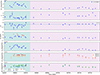 |
Fig. 1. Evolution of spectral parameters and optical–to–X-ray fluxes. From top to bottom: Intrinsic flux in the 0.3–10.0 keV band, photon index, curvature parameter, energy of the SED synchrotron peak and associated flux, and UV (W1, M2 and W2 filters) and optical (V, B and U filters, as well as the VT R and B band) fluxes. The dashed blue line in the β panel represents β = 0.4, considered a threshold value between low and high curvature. The red stars represent unconstrained points whereas red triangle represent 1σ upper limits. The blue and magenta backgrounds highlight periods 1 and 2 respectively. |
We modeled spectra in XSPEC version 12.14.0 using an absorbed log-parabolic model (constant*TBabs*logpar; Wilms et al. 2000; Massaro et al. 2004), where TBabs accounts for Galactic absorption and the log-parabola, describing the intrinsic source spectrum, is defined as
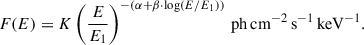 (1)
(1)
We fixed the pivot energy at E1 = 1 keV and the absorption column density at the Galactic value NH = 1.0 × 1021 cm−2 (Kalberla et al. 2005). The log-parabola model is described by three parameters: the photon index at 1 keV (α), the curvature parameter β, and the normalization K. Table B.1 lists the fitted spectral parameters for all observations. Fig. 2 shows an example of a joint fit for the December 16, 2024 observation.
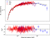 |
Fig. 2. Joint-fit of the XRT, MXT and ECLAIRs spectra for the observations taken on December 16, 2024. Bottom panel: Residuals, computed as the difference between the observed data (D) and the model (M), normalized by the error (σ). |
From these parameters, we followed Massaro et al. (2004) and computed the synchrotron peak energy, Ep, and flux, Sp, as
 (2)
(2)
 (3)
(3)
We propagated uncertainties (68% confidence) on these two parameters from the fit spectral parameters.
Two time periods can be distinguished from the 0.3–10 keV flux and Sp levels. Period 1 (December 6–26, 2024) shows higher fluxes, with weighted means  erg cm−2 s−1 and
  erg cm−2 s−1. Period 2 (January 2–March 1, 2025) shows lower values,
  erg cm−2 s−1 and
  erg cm−2 s−1. We list the weighted mean photon index and curvature,
  and
and  in Table 1, with weights set by the relative uncertainties of the parameters.
Weighted mean values of the curvature parameter and the photon index during periods 1 and 2 and during the total period.
3.2. Spectral analysis
We studied correlations between the parameters using Spearman rank-order correlation coefficients, listed in Table 2. Period 1 is characterized by harder spectra with low curvature ( , the threshold that distinguishes the low- and high-curvature spectra) compared to period 2 (see Table 1). The “harder when brighter” trend noted by Foisseau et al. (2025) is confirmed by the strong anticorrelation between α and the 0.3–10 keV flux (F0.3 − 10 keV) across the full observation campaign (Table 2). Spectra also tend to exhibit lower curvature at higher fluxes, as suggested by an anticorrelation between β and F0.3 − 10 keV. However, this trend is not statistically significant over the two periods.
Spearman correlation coefficients computed for periods 1 and 2 and for the entire period.
A shift of the synchrotron peak energy, Ep, toward higher energies is observed with increasing flux, yielding a positive correlation between Ep and F0.3 − 10 keV in both periods. Such correlations are often accompanied by an anticorrelation between X-ray and radio-to-UV flux, interpreted as a long-term change in the efficiency of the particle acceleration mechanism (Katarzyński et al. 2006; Kapanadze 2018). In our observations, we find no anticorrelation between the X-ray flux and the optical flux in the V band (FV), either within individual periods or in the combined dataset.
The flare does not show significant Ep − β anticorrelation (Table 2) in any period or in the combined dataset. Efficient stochastic acceleration is typically associated with low spectral curvature and a clear Ep − β anticorrelation (Tramacere et al. 2011; Massaro et al. 2011). In our case, only weak indications of this behavior are present, limited to low curvature during period 1 and in the combined dataset (see Table 1).
To further investigate the acceleration processes, we compared the data in the Ep − β plane with theoretical predictions for Fermi I and Fermi II acceleration (Tramacere et al. 2011; Chen 2014), given by ln(Ep) = ln(A)+3/(10β) and ln(Ep) = ln(A)+3/(5β), respectively, with A as a free parameter. Fits to periods 1 and 2 combined yielded poor χ2 values, preventing firm conclusions regarding the dominant acceleration process. Fits on period 1 alone were compatible with both Fermi I and Fermi II scenarios (see Fig. 3). For period 1, the fits resulted in χ2 = 17.9/17 = 1.05 and χ2 = 16.8/17 = 0.99 for the Fermi I and Fermi II scenarios, respectively, while the combined fit to periods 1 and 2 gave χ2 = 104.1/30 = 3.47 and χ2 = 60.9/30 = 2.03 for Fermi I and Fermi II, respectively. We also searched for a positive α − β correlation, expected for Fermi I (Massaro et al. 2004), but found none, either in individual periods or across the full outburst (Table 2).
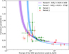 |
Fig. 3. Distribution in the Ep − β plane for the period 1 and 2 combined. Purple and blue lines indicate expectations for Fermi II and Fermi I acceleration, respectively, fit using data from period 1 with an additional multiplicative constant. The colored regions represent 1σ errors. Red stars represent unconstrained points, whereas red triangles represent 1σ upper limits. Errors on Ep at the 1σ level were obtained through error propagation from the 1σ uncertainties on α and β. When the lower bound of the confidence interval included zero, we treated the value as a 1σ upper limit. We also considered values unconstrained when their uncertainties were at least one order of magnitude larger than the measured value itself, and when both limits of the confidence interval were poorly constrained. |
A positive correlation between Ep and Sp is observed (Table 2), which is consistent with stochastic acceleration (Tramacere et al. 2011). Moreover, when the correlation follows Sp ∝ Ep0.6, it further indicates a transition in the turbulence energy spectrum, from a Kraichnan-type regime to a hard-sphere regime (Tramacere et al. 2011; Kapanadze 2018). We fit a power-law model, Sp = C Epq (Fig. 4), finding q = 3.14 ± 2.27, q = 1.17 ± 0.45, and q = 1.29 ± 0.24 for periods 1, 2, and both combined, respectively. Large uncertainties prevent a unique physical interpretation, as the results remain compatible with multiple scenarios (Tramacere et al. 2009).
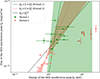 |
Fig. 4. Distribution in the Sp − Ep plane. The dashed line represents Sp ∝ Ep0.6. The orange and green lines represent the model Sp = C × Epq fit to the data from periods 1 and 2, respectively. The colored region represent the 1σ error. Red stars represent unconstrained points, whereas red triangles represent 1σ upper limits. |
Finally, we examined the hardness ratio, HR = F2 − 10 keV/F0.3 − 2 keV (Kapanadze et al. 2018), in the HR − F0.3 − 10 keV plane (Fig. 5). In stochastic acceleration, gradual electron acceleration is expected to produce counter-clockwise (CCW) loops, whereas instantaneous Fermi I acceleration may generate clockwise (CW) loops (see e.g. Cui 2004; Virtanen & Vainio 2005). A visual inspection of Fig. 5 reveals transitions between CW and counterclockwise CCW loops, a behavior commonly observed in HBLs and often interpreted as the result of shocks propagating through jet regions with varying physical conditions (Kapanadze 2018). However, we assessed the statistical significance of these loops (see Appendix C) and found none statistically significant.
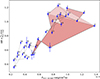 |
Fig. 5. Distribution in the HR − F0.3 − 10 keV plane for the entire follow-up campaign (periods 1 and 2). Numbers near the data points indicate the temporal order (0 to 30). Shaded orange areas represent the three loops initially identified and finally reject by the bootstrap algorithm. The three loops are: 0-6 CW, 0-14 CW, and 0-15 CW. |
4. Discussions and conclusions
On December 6, 2024, the ECLAIRs telescope on board SVOM detected a long X-ray transient spatially coincident with the blazar 1ES 1959+650, marking the first blazar outburst observed by SVOM (Coleiro et al. 2024). Following the trigger, SVOM performed a ToO monitoring campaign until December 26, 2024, capturing the spectral evolution of the source. Swift complemented these observations with 27 pointings from six days after the first detection until March 1, 2025 (Komossa et al. 2024a,b). We modeled the spectral evolution of the source using a log-parabola to identify possible correlations and tentatively probe the flare’s acceleration mechanisms.
The flare exhibits a clear harder-when-brighter trend, along with a shift of the synchrotron peak energy (Ep) toward higher energies, as indicated by the anticorrelation between α and F0.3 − 10 keV and the positive Ep − F0.3 − 10 keV correlation. We detected no corresponding decrease in the optical-to-UV flux during the X-ray rise. We did not clearly detect either Fermi II or Fermi I signatures: fits to theoretical models in the Ep − β plane were inconclusive, and we did not observe a significant α − β correlation. We measured a positive Sp − Ep correlation, consistent with stochastic acceleration, but the exponent remained poorly constrained. Similarly, we identified no significant loops in the HR − F0.3 − 10 keV plane, providing no clear indication of the dominant acceleration process (see Appendix C).
The absence of strong signatures from either Fermi I or Fermi II acceleration suggests that both processes may operate concurrently. Particles could undergo initial shock acceleration followed by stochastic reacceleration downstream, or experience multiple shock crossings (Katarzyński et al. 2006; Petrosian 2012). Consequently, the combination of these mechanisms may weaken individual signatures. Compared to previous flares of 1ES 1959+650, this event does not show clear Fermi-I or Fermi-II dominance, resembling the 2015–2016 outburst (Kapanadze et al. 2016a), whereas other flares showed clearer stochastic acceleration signatures (see e.g. Kapanadze et al. 2018).
This study reports the first blazar outburst detected by SVOM, highlighting the satellite’s and the collaboration’s rapid response, with follow-up observations initiated less than two hours after the trigger. The multiday SVOM campaign, together with Swift, illustrates the potential of the SVOM mission to continuously monitor blazar activity, providing dense temporal and spectral coverage. In particular, the low-energy threshold of ECLAIRs ensures spectral continuity beyond the 10 keV limit covered by XRT and MXT. This yields tighter constraints on physical parameters. Future SVOM observations of 1ES 1959+650, together with multiwavelength facilities will enhance temporal and spectral sampling, offering new opportunities to probe particle acceleration mechanisms in blazar flares.
Acknowledgments
This work was supported by CNES, focused on SVOM. The Space-based multi-band Variable Objects Monitor (SVOM) is a joint Chinese-French mission led by the Chinese National Space Administration (CNSA), the French Space Agency (CNES), and the Chinese Academy of Sciences (CAS). We gratefully acknowledge the unwavering support of NSSC, IAMCAS, XIOPM, NAOC, IHEP, CNES, CEA, CNRS, University of Leicester, and MPE. We would like to thank the Swift team for carrying out the observations we proposed. In addition to our own data, we have also used the Swift archive at https://swift.gsfc.nasa.gov/archive/. SK would like to thank the CAS President’s International Fellowship Initiative for visiting scientists.
References
- Aharonian, F., Akhperjanian, A., Beilicke, M., et al. 2003, A&A, 406, L9 [NASA ADS] [CrossRef] [EDP Sciences] [Google Scholar]
- Baliyan, K. S., Chandra, S., Kaur, N., et al. 2016, ATel, 9070, 1 [Google Scholar]
- Biland, A.& FACT Collaboration 2016, ATel, 9139, 1 [Google Scholar]
- Böttcher, M., Reimer, A., Sweeney, K., & Prakash, A. 2013, ApJ, 768, 54 [Google Scholar]
- Braden, B. 1986, Coll. Math. J., 17, 326 [Google Scholar]
- Buson, S., Magill, J. D., Dorner, D., et al. 2016, ATel, 9010, 1 [Google Scholar]
- Cardelli, J. A., Clayton, G. C., & Mathis, J. S. 1989, ApJ, 345, 245 [Google Scholar]
- Chen, L. 2014, ApJ, 788, 179 [NASA ADS] [CrossRef] [Google Scholar]
- Coleiro, A., Maggi, P., Götz, D., et al. 2024, ATel, 16935, 1 [Google Scholar]
- Cui, W. 2004, ApJ, 605, 662 [Google Scholar]
- Daniel, M. K., Badran, H. M., Bond, I. H., et al. 2005, ApJ, 621, 181 [Google Scholar]
- Dermer, C. D., Schlickeiser, R., & Mastichiadis, A. 1992, A&A, 256, L27 [NASA ADS] [Google Scholar]
- Elvis, M., Plummer, D., Schachter, J., & Fabbiano, G. 1992, ApJS, 80, 257 [CrossRef] [Google Scholar]
- Fan, X., Zou, G., Wei, J., et al. 2020, SPIE Conf. Ser., 11443, 114430Q [Google Scholar]
- Foisseau, A., Cangemi, F., Coleiro, A., et al. 2025, ATel, 16978, 1 [Google Scholar]
- Gehrels, N., Chincarini, G., Giommi, P., et al. 2004, ApJ, 611, 1005 [Google Scholar]
- Godet, O., Nasser, G., Atteia, J., et al. 2014, SPIE Conf. Ser., 9144, 914424 [Google Scholar]
- Götz, D., Boutelier, M., Burwitz, V., et al. 2023, Exp. Astron., 55, 487 [CrossRef] [Google Scholar]
- Gregory, P. C., & Condon, J. J. 1991, ApJS, 75, 1011 [Google Scholar]
- Halzen, F., & Hooper, D. 2005, Astropart. Phys., 23, 537 [Google Scholar]
- Holder, J., Bond, I. H., Boyle, P. J., et al. 2003, ApJ, 583, L9 [Google Scholar]
- Kalberla, P. M. W., Burton, W. B., Hartmann, D., et al. 2005, A&A, 440, 775 [NASA ADS] [CrossRef] [EDP Sciences] [Google Scholar]
- Kapanadze, B. 2018, Galaxies, 6, 125 [Google Scholar]
- Kapanadze, B., Dorner, D., Vercellone, S., et al. 2016a, MNRAS, 461, L26 [NASA ADS] [CrossRef] [Google Scholar]
- Kapanadze, B., Romano, P., Vercellone, S., et al. 2016b, MNRAS, 457, 704 [NASA ADS] [CrossRef] [Google Scholar]
- Kapanadze, B., Dorner, D., Vercellone, S., et al. 2018, ApJS, 238, 13 [NASA ADS] [CrossRef] [Google Scholar]
- Katarzyński, K., Ghisellini, G., Mastichiadis, A., Tavecchio, F., & Maraschi, L. 2006, A&A, 453, 47 [NASA ADS] [CrossRef] [EDP Sciences] [Google Scholar]
- Komossa, S., Grupe, D., Wei, J. Y., & Xu, D. W. 2024a, ATel, 16941, 1 [Google Scholar]
- Komossa, S., Grupe, D., Wei, J. Y., et al. 2024b, ATel, 16955, 1 [Google Scholar]
- Krawczynski, H., Hughes, S. B., Horan, D., et al. 2004, ApJ, 601, 151 [NASA ADS] [CrossRef] [Google Scholar]
- Marscher, A. P., & Gear, W. K. 1985, ApJ, 298, 114 [Google Scholar]
- Massaro, E., Perri, M., Giommi, P., & Nesci, R. 2004, A&A, 413, 489 [NASA ADS] [CrossRef] [EDP Sciences] [Google Scholar]
- Massaro, F., Paggi, A., & Cavaliere, A. 2011, ApJ, 742, L32 [NASA ADS] [CrossRef] [Google Scholar]
- Nishiyama, T. 1999, Int. Cosm. Ray Conf., 3, 370 [Google Scholar]
- Petrosian, V. 2012, Space Sci. Rev., 173, 535 [NASA ADS] [CrossRef] [Google Scholar]
- Tramacere, A., Giommi, P., Perri, M., Verrecchia, F., & Tosti, G. 2009, A&A, 501, 879 [NASA ADS] [CrossRef] [EDP Sciences] [Google Scholar]
- Tramacere, A., Massaro, E., & Taylor, A. M. 2011, ApJ, 739, 66 [Google Scholar]
- Urry, C. M., & Padovani, P. 1995, PASP, 107, 803 [NASA ADS] [CrossRef] [Google Scholar]
- Virtanen, J. J. P., & Vainio, R. 2005, AIP Conf. Ser., 801, 410 [Google Scholar]
- Wei, J., Cordier, B., Antier, S., et al. 2016, arXiv e-prints [arXiv:1610.06892] [Google Scholar]
- Wilms, J., Allen, A., & McCray, R. 2000, ApJ, 542, 914 [Google Scholar]
Appendix A: Instruments and data reduction
A.1. The SVOM space mission
SVOM has discovered 1ES 1959+650 on December 6, 2024, in an outburst phase with the ECLAIRs telescope (Coleiro et al. 2024) onboard the satellite. The outburst phase of 1ES 1959+650 has then been followed through the Target of Opportunity (ToO) program until December 26, 2024 Foisseau et al. (2025), see Table A.1). Because of solar constraints, SVOM has not been able to observe the entire flaring phase. Note that the observations have been performed during the commissioning and verification phase of SVOM.
A.1.1. The ECLAIRs (4–150 keV) instrument
The ECLAIRs telescope (Godet et al. 2014, Godet et al. in prep) is a coded mask instrument with a large field of view (FoV) of ∼2 sr, operating in the 4–150 keV energy band. The data have been reduced using the official pipeline, namely ECPI version 1.15.1 (Goldwurm et al. in prep), with the calibration files from version 20240101.
The ECPI pipeline reduces the ECLAIRs data based on the following steps. Good Time Intervals (GTIs) are defined, and energy calibration of the events is performed by applying a pixel gain and offset, while events that are not valid are flagged. Binned detector images are then created and corrected for efficiency, non-uniformity, and background. Sky images are finally reconstructed through deconvolution and coding-noise cleaning. Based on the source position in the sky images, ECPI builds a specific shadowgram model, which is fitted to the detector maps to extract the flux in each energy bin, while a second-degree polynomial accounts for the background component.
We considered all the observations in which 1ES 1959+650 was detected. For each observation considered, a spectrum was produced with 15 bins logarithmically distributed over the entire ECLAIRs energy band. The response matrix file and the ancillary response file used were respectively ECL-RSP-RMF_20220515T01.fits and ECL-RSP-ARF_20220515T01.fits. To increase the signal-to-noise ratio of the spectrum, we then combined the spectra from observations taken on the same day.
A.1.2. The MXT (0.3–10 keV) instrument
The MXT telescope (Microchannel X-ray Telescope, Götz et al. 2023, Götz et al. in prep) has a 58 × 58 arcmin squared FoV, operating in the 0.3–10 keV energy band. For every observation, the data have been reduced and the spectra produced using the official pipeline, called MXT-pipeline (Maggi et al. in prep), in its 1.9.0 version. The response matrix file and ancillary response file used in the analysis were MXT-GND-MATRIX-ALL_20250206T093900_20240315113300.2.fits and MXT_FM_PANTER_FULL-ALL-1.1.arf. The background file used was produced with the MXT-pipeline task. Because of instrumental calibration issues, we chose to consider the data only above 1.0 keV. Also, to ensure the possibility of using the Gaussian approximation, we binned the spectra with at least 50 cts/bin using ftgrouppha, developed as part of the HEASoft suite.
A.1.3. The VT optical telescope
The VT telescope (Visible Telescope, Fan et al. 2020, Qiu et al. in prep) is an optical telescope (40 cm aperture size) operating with two filters: the VTB (400–650 nm) and VTR (650–1000 nm) bands, with a field of view (FoV) of 26’ in diameter. The data were analyzed following the standard procedure. 1ES 1959+650 has been observed by the VT only for two observations, taken on December 6 and December 26, 2024 (Foisseau et al. 2025).
The magnitudes were measured in the AB reference system. They were corrected for extinction following Cardelli et al. (1989). The corrected magnitudes were then converted into energy fluxes by adopting effective wavelengths of λR = 789.6 ± 94.0 nm and λB = 533.7 ± 78.5 nm for the R and B filters, respectively. Flux uncertainties were computed via error propagation, taking into account the uncertainties on the magnitudes as well as on the reference wavelengths for each filter. An error of 5% has been assumed on the magnitude values (internal communication).
A.2. SVOM trigger and alert system
On Friday, December 6 at 15:08:48 UT (Tb), the on-board trigger software of the ECLAIRs telescope detected and localized a long-duration soft X-ray transient at RA = 300.202°, DEC = 65.182° (J2000). The source position is constrained within a 9.3 arcmin uncertainty radius in the 5–8 keV energy band, during a 22-min exposure starting at Tb. A subsequent alert with SNR = 7.2 was issued in the same band during an 11-minute exposure beginning at 15:14:15 UT. The sub-image transmitted in near real-time via the SVOM VHF network revealed a clear point-like source absent from the on-board catalog.
Following this trigger, a Target of Opportunity (ToO) observation with MXT and VT was carried out at 16:47:41 UT, with an exposure of 3.6 ks. A single source was detected at RA = 300.0125°, DEC = 65.1519° (J2000), with a positional uncertainty of 25 arcsec (90% confidence level). This source lies 22 arcsec from the BL Lac blazar 1ES 1959+650.
A.3. The Swift Neil Gehrels Observatory
1ES 1959+650 was followed up with the Neil Gehrels Swift Observatory (Gehrels et al. 2004) in the period December 12, 2024 to March 01, 2025, starting 6 days after the initial SVOM discovery of the X-ray outburst (Komossa et al. 2024a,b, see Table A.1). In addition to our own Swift follow-ups, we also analyzed archival Swift observations from that epoch. For comparison with the ongoing outburst, we also analyzed earlier Swift observations from August 2024 when the blazar was found to be in its intermediate-to-low state.
A.3.1. The XRT (0.3–10 keV) telescope
The Swift X-ray telescope (XRT) observations were carried out in windowed timing (WT) mode because of the high X-ray count rate. Data were reduced with the XRTPIPELINE 0.13.7, that is part of the HEASoft package 6.35.1. For spectral analysis the response file swxwt0s6_20210101v016.rmf was used. Source counts were extracted in a rectangular region of radius 40x3 pixels. Source spectra of each epoch were produced and fitted with a single powerlaw model with absorption fixed at the Galactic value of 1.0 × 1021 cm−2 (Kalberla et al. 2005), and free photon index Γ.
During the Swift observations, the X-ray count rate varied by a factor ∼4.6 and the peak flux was reached on December 16, 2024. A very strong anticorrelation between X-ray flux and spectral index Γ is immediately evident (see Fig. A.1). For further analysis, the Swift/XRT and SVOM X-ray data were combined. For the following analysis, to ensure the possibility to use a Gaussian approximation, we binned the spectra with at least 50 cts/bin using ftgrouppha.
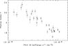 |
Fig. A.1. Power-law photon index Γ as function of the 0.3-10 keV flux of the XRT observations of 1ES 1959+650 between August 2024 and March 2025. The Spearman correlation coefficient ρ = −0.89 determined with a p-value p = 5 × 10⁻¹¹. |
A.3.2. The UVOT (UV/optical) telescope
1ES 1959+650 was also observed with the Swift UV-optical telescope (UVOT) in all three optical and three UV filters in order to ensure good SED coverage of this highly variable blazar. The UVOT data of each segment were co-added using the task UVOTIMSUM. Source counts were extracted in a circular region of radius 5 arcseconds. UVOT magnitudes were measured following standard procedures and were corrected for Galactic extinction based on Cardelli et al. (1989). The optical–UV emission was also found to be in a high state. However, it did not closely follow the X-ray evolution. The optical maximum was reached on January 31, 2025, which is 56 days after the observed X-ray peak on December 6, 2024.
Summary of the joint-observation campaign of SVOM and Swift for the outburst phase of 1ES 1959+650 from December 6, 2024 to March 01, 2025.
Appendix B: Long-term spectral parameter evolution
Table B.1 provides the fitted spectral parameters for each dataset considered in our work. As explained in Section 3.1, the outburst phase can be divided into two distinct periods. The first period (2024 December 6–26), covered by both SVOM and Swift, shows a high flux level in the 0.3–10 keV band ( erg cm−2 s−1), with a hard spectrum combined with low curvature (
 , see Table 1). In contrast, the second period (2025 January 2–March 1), covered solely by Swift, exhibits a lower spectral flux in the same energy band (
 erg cm−2 s−1), along with a softer spectrum and higher curvature (
 ). Meanwhile, the optical and UV fluxes, computed in the V and W1 bands respectively, show slightly higher values during period 2 (
 erg cm−2 s−1 and
  erg cm−2 s−1) compared to period 1 (
 erg cm−2 s−1 and
  erg cm−2 s−1).
Spectral parameters.
Appendix C: Search for hysteresis in the HR − F0.3 − 10 keV plane
To quantify the presence of loops in the HR − F0.3 − 10 keV plane, we computed the area enclosed by successive time-ordered observations. The area was calculated using the Gauss (shoelace) formula (Braden 1986). Each loop was required to contain at least three points. For the i-th loop, defined by observations with indices ranging from kmin to kmax, the enclosed area is given by
 (C.1)
(C.1)
With this convention, negative (positive) areas correspond to CW (CCW) rotations. Applying this method to all possible sequences yielded 435 candidate loops. To assess their statistical significance, we performed 10,000 bootstrap simulations by randomizing the observation indices. The resulting distributions of simulated loop areas showed that none of the observed loops exceed a significance of 3σ.
All Tables
Weighted mean values of the curvature parameter and the photon index during periods 1 and 2 and during the total period.
Spearman correlation coefficients computed for periods 1 and 2 and for the entire period.
Summary of the joint-observation campaign of SVOM and Swift for the outburst phase of 1ES 1959+650 from December 6, 2024 to March 01, 2025.
All Figures
|
Fig. 1. Evolution of spectral parameters and optical–to–X-ray fluxes. From top to bottom: Intrinsic flux in the 0.3–10.0 keV band, photon index, curvature parameter, energy of the SED synchrotron peak and associated flux, and UV (W1, M2 and W2 filters) and optical (V, B and U filters, as well as the VT R and B band) fluxes. The dashed blue line in the β panel represents β = 0.4, considered a threshold value between low and high curvature. The red stars represent unconstrained points whereas red triangle represent 1σ upper limits. The blue and magenta backgrounds highlight periods 1 and 2 respectively. |
| In the text | |
|
Fig. 2. Joint-fit of the XRT, MXT and ECLAIRs spectra for the observations taken on December 16, 2024. Bottom panel: Residuals, computed as the difference between the observed data (D) and the model (M), normalized by the error (σ). |
| In the text | |
|
Fig. 3. Distribution in the Ep − β plane for the period 1 and 2 combined. Purple and blue lines indicate expectations for Fermi II and Fermi I acceleration, respectively, fit using data from period 1 with an additional multiplicative constant. The colored regions represent 1σ errors. Red stars represent unconstrained points, whereas red triangles represent 1σ upper limits. Errors on Ep at the 1σ level were obtained through error propagation from the 1σ uncertainties on α and β. When the lower bound of the confidence interval included zero, we treated the value as a 1σ upper limit. We also considered values unconstrained when their uncertainties were at least one order of magnitude larger than the measured value itself, and when both limits of the confidence interval were poorly constrained. |
| In the text | |
|
Fig. 4. Distribution in the Sp − Ep plane. The dashed line represents Sp ∝ Ep0.6. The orange and green lines represent the model Sp = C × Epq fit to the data from periods 1 and 2, respectively. The colored region represent the 1σ error. Red stars represent unconstrained points, whereas red triangles represent 1σ upper limits. |
| In the text | |
|
Fig. 5. Distribution in the HR − F0.3 − 10 keV plane for the entire follow-up campaign (periods 1 and 2). Numbers near the data points indicate the temporal order (0 to 30). Shaded orange areas represent the three loops initially identified and finally reject by the bootstrap algorithm. The three loops are: 0-6 CW, 0-14 CW, and 0-15 CW. |
| In the text | |
|
Fig. A.1. Power-law photon index Γ as function of the 0.3-10 keV flux of the XRT observations of 1ES 1959+650 between August 2024 and March 2025. The Spearman correlation coefficient ρ = −0.89 determined with a p-value p = 5 × 10⁻¹¹. |
| In the text | |
Current usage metrics show cumulative count of Article Views (full-text article views including HTML views, PDF and ePub downloads, according to the available data) and Abstracts Views on Vision4Press platform.
Data correspond to usage on the plateform after 2015. The current usage metrics is available 48-96 hours after online publication and is updated daily on week days.
Initial download of the metrics may take a while.