| Issue |
A&A
Volume 705, January 2026
|
|
|---|---|---|
| Article Number | A72 | |
| Number of page(s) | 11 | |
| Section | Interstellar and circumstellar matter | |
| DOI | https://doi.org/10.1051/0004-6361/202557102 | |
| Published online | 07 January 2026 | |
CO depletion in infrared dark clouds
1
Institut de Radioastronomie Millimétrique,
300 Rue de la Piscine,
38400
Saint-Martin-d’Hères,
France
2
European Southern Observatory,
Karl-Schwarzschild-Strasse 2,
85748
Garching,
Germany
3
Department of Space, Earth and Environment, Chalmers University of Technology,
412 96
Gothenburg,
Sweden
4
Department of Astronomy, University of Virginia,
530 McCormick Road,
Charlottesville,
VA
22904-4325,
USA
5
Department of Astronomy, Yale University,
New Haven,
CT
06511,
USA
6
INAF Osservatorio Astronomico di Arcetri,
Largo E. Fermi 5,
50125
Florence,
Italy
7
California Institute of Technology,
Pasadena,
CA
91125,
USA
8
Centro de Astrobiología (CSIC/INTA),
Ctra. de Torrejón a Ajalvir km 4,
Madrid,
Spain
9
Laboratory for the study of the Universe and eXtreme phenomena (LUX),
Observatoire de Paris, 5, place Jules Janssen,
92195
Meudon,
France
10
Max Planck Institute for Extraterrestrial Physics,
Giessenbachstrasse 1,
85748
Garching bei München,
Germany
11
Astrophysics Research Institute, Liverpool John Moores University,
146 Brownlow Hill,
Liverpool
L3 5RF,
UK
12
Leiden Observatory, Leiden University,
PO Box 9513,
2300 RA
Leiden,
The Netherlands
★ Corresponding author: This email address is being protected from spambots. You need JavaScript enabled to view it.
Received:
4
September
2025
Accepted:
28
October
2025
Abstract
Context. Infrared dark clouds (IRDCs) are cold, dense structures that are likely representative of the initial conditions of star formation. Many studies of IRDCs employ CO to investigate cloud dynamics, but CO can be highly depleted from the gas phase in IRDCs, which affects its fidelity as tracer. The CO depletion process is also of great interest in astrochemistry because CO ice in dust grain mantles provides the raw material for the formation of complex organic molecules.
Aims. We study CO depletion towards four IRDCs to investigate its correlation with the H2 number density and dust temperature, calculated from Herschel far-infrared images.
Methods. We used 13CO J = 1 → 0 and 2 → 1 maps to measure the CO depletion factor, fD, across IRDCs G23.46-00.53, G24.49-00.70, G24.94-00.15, and G25.16-00.28. We also considered a normalised CO depletion factor, f′D, which takes a value of unity, that is, no depletion, in the outer lower-density and warmer regions of the clouds. We then investigated the dependence of fD and f′D on the gas density, nH, and dust temperature, Tdust.
Results. The CO depletion rises as the density increases and reaches maximum values of f′D ∼ 10 in some regions with nH ≳ 3 × 105 cm−3, although with significant scatter at a given density. We find a tighter, less scattered relation of f′D with temperature that rapidly rise for temperatures ≲18 K. We propose a functional form f′D = exp(T0/[Tdust − T1]) with T0 ≃ 4 K and T1 ≃ 12 K to reproduce this behaviour.
Conclusions. We conclude that CO is strongly depleted from the gas phase in cold, dense regions of IRDCs. This means that if it is not accounted for, CO depletion can lead to an underestimation of the total cloud masses based on CO line fluxes by factors up to ∼5. These results indicate a dominant role for thermal desorption in setting near equilibrium abundances of gas-phase CO in IRDCs and provide important constraints for astrochemical models and the chemodynamical history of gas in the early stages of star formation.
Key words: ISM: abundances / ISM: clouds / ISM: kinematics / dynamics / ISM: lines / bands / ISM: molecules
© The Authors 2026
 Open Access article, published by EDP Sciences, under the terms of the Creative Commons Attribution License (https://creativecommons.org/licenses/by/4.0), which permits unrestricted use, distribution, and reproduction in any medium, provided the original work is properly cited.
This article is published in open access under the Subscribe to Open model. This email address is being protected from spambots. You need JavaScript enabled to view it. to support open access publication.
1 Introduction
Infrared dark clouds (IRDCs) are cold (T ≲ 20 K; Pillai et al. 2006), dense (nH ≳ 104 cm−3; Butler & Tan 2012) and highly extincted (AV ∼ 10–100 mag) regions of the interstellar medium (ISM) that are known to harbour the conditions of star and star cluster formation. First detected as dark features against the mid-infrared (MIR) Galactic background (Perault et al. 1996; Egan et al. 1998), IRDCs show low levels of star formation activity, and their mass surface densities are similar to those of massive star-forming regions (Tan et al. 2014). Furthermore, IRDCs host cold, dense, deuterated pre-stellar cores, that is, the earliest phase of massive star formation (Tan et al. 2013; Kong et al. 2017). For all these reasons, IRDCs have long been regarded as the birth places of massive stars and star clusters (Rathborne et al. 2006; Foster et al. 2014; Pillai et al. 2019; Moser et al. 2020; Yu et al. 2020).
Despite this importance, the mechanisms that trigger star formation in these objects are still unclear (e.g. Tan 2000; Tan et al. 2014; Hernandez & Tan 2015; Peretto et al. 2016; Retes-Romero et al. 2020; Morii et al. 2021). Theoretical models and simulations have suggested that star formation can be efficiently ignited within IRDCs as a consequence of dynamical compression and gravitational instability of the gas. In current theories, IRDCs have been proposed to form as the shock-compressed layer in the collision between pre-existing giant molecular clouds (GMCs; e.g. Tan 2000; Tasker & Tan 2009; Tan 2010; Suwannajak et al. 2014; Wu et al. 2015, 2017; Li et al. 2018; Fortune-Bashee et al. 2024), with the collision being a consequence of the GMC orbital motion in a shearing Galactic disk. Other models also involve the formation from compressive collisions, but driven by momentum from stellar feedback (e.g. Inutsuka et al. 2015). Still other models invoke the IRDCs and dense clump formation as part of the same processes of hierarchical gravitational collapse that forms the surrounding GMCs (e.g. Vázquez-Semadeni et al. 2019). All these mechanisms are expected to leave different imprints on the gas dynamical properties in the formed IRDCs.
Since molecular hydrogen H2, the primary constituent of molecular clouds, is not excited at the low temperatures of these objects, indirect methods of tracing cloud mass have been developed. Among these, CO rotational transitions and its isotopologues have been used to study the structure and kinematics of molecular clouds, assuming a certain CO to H2 abundance ratio. For the conditions that typically prevail in IRDCs, however, CO can be strongly depleted in the gas phase by freeze-out onto dust grains (e.g. Caselli et al. 1999; Crapsi et al. 2005; Fontani et al. 2006; Hernandez et al. 2011; Jiménez-Serra et al. 2014; Sabatini et al. 2019; Entekhabi et al. 2022). This may cause important quantities, such as cloud mass, to be significantly underestimated.
CO depletion also has major implications for the chemistry of star-forming regions. For example, if CO is highly depleted from the gas phase, then the abundance of H2D+ can rise, which leads to high levels of deuteration of the remaining gas-phase species, such as N2H+ and NH3 (e.g. Dalgarno & Lepp 1984; Caselli et al. 2002; Fontani et al. 2006; Caselli et al. 2008; Kong et al. 2015; Sabatini et al. 2020, 2024; Redaelli et al. 2021; Entekhabi et al. 2022; Redaelli et al. 2022). In addition, the formation of many complex organic molecules (COMs) is expected to occur within the CO ice mantles of dust grains (e.g. Herbst & van Dishoeck 2009).
The gas-phase depletion of CO is typically quantified using the so-called CO depletion factor, fD, that is, the ratio of the expected CO column density given a CO-independent measure of the column density of H nuclei, NH, and assuming the standard gas-phase CO abundance along a line of sight to the observed CO column density. Estimates of NH in molecular clouds are typically made via dust continuum emission at sub-millimetre and millimetre wavelengths (e.g. Lim et al. 2016) or via mid- and near-infrared (NIR) dust extinction measurements (e.g. Butler & Tan 2012; Kainulainen & Tan 2013).
On the smaller scales of cores (≲0.1 pc), CO depletion has been investigated towards low- (e.g. Caselli et al. 1999; Kramer et al. 1999; Whittet et al. 2010; Ford & Shirley 2011; Christie et al. 2012) and high-mass (e.g. Fontani et al. 2006; Zhang et al. 2009; Fontani et al. 2012; Sabatini et al. 2019) examples. In both cases, high values of CO depletion factors have been reported. In particular, in high-mass pre-stellar and early-stage cores, Fontani et al. (2012) estimated values up to fD > 80, while Zhang et al. (2009) found fD > 100. High angular resolution observations obtained with the Atacama Large millimeter/sub-millimeter array (ALMA) of massive clumps and cores from the ASHES survey by Sabatini et al. (2022) showed CO depletion factors up to ≳100 that did not decrease from the pre-stellar to the protostellar cores.
On the larger scales of IRDCs, Hernandez et al. (2011) and Hernandez et al. (2012) used multi-transition single-dish observations of the C18O isotope to obtain a parsec-scale CO depletion map of IRDC G35.39-00.33. Under the assumption of local thermodynamic equilibrium (LTE) conditions, they reported values of fD of up to ∼3. Towards the same cloud, Jiménez-Serra et al. (2014) used the LVG approximation and reported CO depletion factors of ∼5, 8, and 12 in three selected positions. Similar results were reported towards IRDC G351.77-0.51 by Sabatini et al. (2019). Towards IRDC G28.37+00.07, Entekhabi et al. (2022) reported values of fD up to ∼10. Feng et al. (2020) investigated CO depletion towards a sample of four IRDCs and presented CO depletion maps with fD values of up to 15. Towards the Serpens filament, Gong et al. (2021) reported widespread CO depletion, suggesting that the filament is young and still accreting. On larger scales, Clarke et al. (2024) reported CO depletion towards the giant molecular filament G214.5−1.8 already at volume densities 2 × 103 cm−3, which translates into a very low cosmic-ray ionisation rate (ζ ≈ 2 × 10⁻¹⁸ s−1). Similarly, Hirata et al. (2024) observed parsec-scale CO depletion towards several star-forming regions associated with Canis Major OB1. The authors showed that C18O(1–0) under-traces dense gas at parsec scales, although it remains unclear to which extent local temperature conditions affect this behaviour. Finally, Socci et al. (2024) investigated the large-scale CO depletion across OMC-2 and OMC-3 and reported values that are consistent with previous measurements obtained in star-forming regions. The authors also suggested CO depletion as a viable proxy of o-H2D+. All these studies have confirmed that depletion of CO from the gas phase is significant not just towards the dense cores and clumps, but also in the inter-clump regions of IRDCs.
While it is generally known that CO depletion is affected by density and temperature variations, only a few previous studies have been dedicated to specific investigation of the dependence of fD on these properties. In particular, Kramer et al. (1999) investigated the dependence of CO depletion on the dust temperature towards the dense core IC 5146. They found that their data were well fitted with the following function:
 (1)
with
(1)
with  and T0 = 14.1 ± 0.6 K. We note, however, that their data covered a relatively modest range of depletion factors, that is, up to fD ∼ 2.5. Furthermore, their dust temperatures were estimated based on the ratio of 1.2 mm flux to NIR dust extinction (with equivalent AV ranging up to about 30 mag, i.e. up to Σ ≃ 0.13 g cm−2), which is relatively sensitive to the choice of dust opacity model.
In this work, we explore CO depletion in a sample of four IRDCs, namely G24.94-00.15, G23.46-00.53, G24.49-00.70, G25.16-00.28, which are part of a larger sample of 26 clouds (Butler & Tan 2009, 2012, Cosentino et al., in prep.). This paper is organised as follows. In Section 2 we present our sample, the data, and the technical details of our observations. In Section 3, we describe the method we adopted and the analysis we performed. In Sections 4 and 5, we present and discuss our results. In Section 6 we draw our conclusions.
2 The IRDC sample
The four IRDCs studied in this work were selected from a larger sample of 16 clouds (K to Z) that will be presented in a forthcoming paper (Cosentino et al. in prep.). They extend the sample of ten IRDCs of Butler & Tan (2009, 2012) (labelled A to J). These 26 sources were identified as dark features against the diffuse MIR Galactic background. They were selected for being located relatively nearby (kinematic distance ≤7 kpc) and for showing the highest levels of contrast against the diffuse Galactic background emission as observed with Spitzer-IRAC at 8 µm (Churchwell et al. 2009).
We selected the four IRDCs, namely G24.94-00.15 (cloud O), G23.46-00.53 (cloud V), G24.49-0.70 (cloud X), and G25.16-0.28 (cloud Y) to probe different regimes of the mass surface density, Σ, and dust temperature, Tdust. In addition, these IRDCs show relatively simple kinematics (Cosentino et al., in prep.). For the four clouds, Σ and Tdust images were obtained from multi-wavelength Herschel images using the method described by Lim et al. (2016). Briefly, Herschel-PACS and SPIRE images at 160, 250, 350, and 500 µm were first re-gridded to match the poorest angular resolution of the 500 µm image (36″). Next, the Galactic Gaussian method of background subtraction was used (see Lim et al. 2016). The effect of this is to remove ∼0.1 g cm2 and ∼2 K from all clouds on average in the Σ and Tdust images, respectively. After this, the multi-wavelength emission, re-gridded to a scale of 18″ pixels (hires method of Lim et al. 2016), was fitted using a grey body function, and Σ and Tdust were estimated. The Σ and Tdust Herschel-derived images of the four clouds are shown in Figure 1. For each cloud, the average subtracted background, average Σ, and Tdust noise values are reported in Table 1. To the best of our knowledge, no previous studies have been dedicated to these clouds.
Noise and background values for the Herschel-derived Σ and Tdust.
3 Observations and data
In May 2021, we used the 30m single-dish antenna at the Instituto de Radioastronomia Millimetrica (IRAM 30m; Pico Veleta, Spain) to map the J = 2 →1 rotational transition of 13CO (ν=220.38 GHz) towards 16 IRDCs as an extension of the A-J sample of Butler & Tan (2012). The observations were performed in on-the-fly observing mode with an angular separation in the direction perpendicular to the scanning direction of 6″. For each cloud, the central map coordinates, the map size, and the off positions are listed in Table 2. For the observations, we used the Fast Fourier transform spectrometer (FTS) set to provide a spectral resolution of 50 kHz, corresponding to a velocity resolution of 0.13 km s−1 at the 13CO(2–1) rest frequency. The intensities were measured in units of antenna temperature,  , and converted into main-beam brightness temperature,
  , using forward and beam efficiencies of Feff and Beff of 0.94 and 0.61, respectively1. The final data cubes were created using the CLASS software within the GILDAS2 package and have a spatial resolution of 11″ and a pixel size of 5.5″ × 5.5″. The achieved rms per channel per pixel is reported in Table 2.
The 13CO(2–1) IRAM30m data were complemented using the 13CO(1–0) cubes from the FOREST Unbiased Galactic plane Imaging survey with the Nobeyama 45-m telescope (FUGIN) survey (Umemoto et al. 2017). This survey uses the 45m antenna at the Nobeyama Radio Observatory (Japan) to map the 12CO, 13CO and C18O J = 1 →0 transitions towards part of the first (10◦ ≤ l ≤ 50◦, |b| ≤ 1◦) and third (198◦ ≤ l ≤ 236◦, |b| ≤ 1◦) quadrants of the Galaxy. The observations were performed in on-the-fly mode with a scanning speed of 100″/s. The publicly available cubes have Beff=0.43, an angular resolution of 20″, a pixel size of 8.5″, a velocity resolution of 0.65 km s−1, and an rms of 0.65 K per channel per pixel. For a more detailed description of the survey, we refer to Umemoto et al. (2017).
4 Results and discussion
4.1 Identification of the 13CO emission velocity
In Figure 2 (left column), we show the 13CO(1–0) (black) and (2–1) (red) spectra averaged across the full map regions of each IRDC. Most spectra show multiple velocity components in both transitions. 13CO is a very abundant species (χ ∼10−6 with respect to H; e.g. Frerking et al. 1982) that probes relatively low-density molecular material in the ISM (the typical critical densities of the J=1–0 transition is ∼103 cm−3; Yang et al. 2010). We now wish to discern which of these components are associated with the clouds and which simply arise from emission along the line of sight. To do this, we visually investigated the spatial correspondence and overlap between the cloud structure seen in the Herschel-derived maps (Figure 1) and each velocity component. From this correspondence, we identified the velocity ranges of the 13CO emission associated with each cloud to be in the ranges 40–60 km s−1 for G24.94-00.15, 58–68 km s−1 for G23.46-00.53, 42–54 km s−1 for G24.49-00.70, and 58–68 km s−1 for G25.16-00.28. The 13CO(1–0) and (2–1) integrated intensity maps obtained over these velocity ranges are also shown in Figure 2. These velocity ranges are reported in Table 2, along with the corresponding integrated noise for both transitions. We note that a more detailed analysis of the gas kinematics towards these sources will be presented in a forthcoming paper.
4.2 Σ13CO and Tex maps
Following the method described by Hernandez et al. (2011), we used the 13CO(1–0) and (2–1) emission to map the CO depletion factor across the four clouds. In particular, we re-gridded the 13CO(2–1) IRAM maps to match the poorer pixel size and the angular and velocity resolution of the corresponding 13CO(1–0) FUGIN maps. We then assumed local thermodynamic equilibrium (LTE) conditions and used the following Equation (see Eq. (A4) of Caselli et al. 2002) to estimate the column density of the species:
![Mathematical equation: ${{d{N^{^{13}{\rm{CO}}}}(v)} \over {dv}} = {{8\pi {v^3}} \over {{c^3}{A_{ul}}}}{{{g_l}} \over {{g_u}}}{{{Q_{{\rm{rot}}}}\left( {{T_{{\rm{ex}}}}} \right)} \over {1 - \exp \left( { - hv/\left[ {k{T_{ex}}} \right]} \right)}}{{{\tau _v}} \over {{g_l}\exp \left( { - {E_l}/\left[ {k{T_{ex}}} \right]} \right)}},$](/articles/aa/full_html/2026/01/aa57102-25/aa57102-25-eq10.png) (2)
where ν is the frequency of the transition, that is, 110.2 GHz and 220.4 GHz for 13CO(1–0) and (2–1) respectively, Aul is the Einstein coefficient for spontaneous emission (6.3324 × 10⁻⁸ s−1 for J = 1 →0 and 6.0745 × 10⁻⁷ s−1 for J = 2 →1), gl and gu are the statistical weights of the lower and upper levels, respectively, Qrot is the rotational partition function, El is the energy of the lower state in the transition, and τ is the optical depth. All spectroscopic parameters were obtained from the catalogue of the Cologne Database for Molecular Spectroscopy3 and are listed in Table 3 (except for gl, which cancels out in Eq. (2)). We used the following expression for Qrot:
(2)
where ν is the frequency of the transition, that is, 110.2 GHz and 220.4 GHz for 13CO(1–0) and (2–1) respectively, Aul is the Einstein coefficient for spontaneous emission (6.3324 × 10⁻⁸ s−1 for J = 1 →0 and 6.0745 × 10⁻⁷ s−1 for J = 2 →1), gl and gu are the statistical weights of the lower and upper levels, respectively, Qrot is the rotational partition function, El is the energy of the lower state in the transition, and τ is the optical depth. All spectroscopic parameters were obtained from the catalogue of the Cologne Database for Molecular Spectroscopy3 and are listed in Table 3 (except for gl, which cancels out in Eq. (2)). We used the following expression for Qrot:
![Mathematical equation: ${Q_{{\rm{rot}}}} = \mathop \sum \limits_{J = 0}^\infty (2J + 1)\exp \left( { - {E_J}/\left[ {k{T_{ex}}} \right]} \right),$](/articles/aa/full_html/2026/01/aa57102-25/aa57102-25-eq11.png) (3)
with EJ = J(J + 1)hB, where B is the 13CO rotational constant 55101.011 MHz4.
(3)
with EJ = J(J + 1)hB, where B is the 13CO rotational constant 55101.011 MHz4.
The optical depth, τν, in Eq. (2) was estimated via
![Mathematical equation: ${T_{B,v}} = {{hv} \over k}\left[ {f\left( {{T_{ex}}} \right) - f\left( {{T_{bg}}} \right)} \right]\left( {1 - {e^{ - {\tau _v}}}} \right).$](/articles/aa/full_html/2026/01/aa57102-25/aa57102-25-eq15.png) (4)
(4)
Here, TB,ν is the main-beam brightness temperature at each velocity (or frequency), f (T) ≡ exp(hν/[kT]) – 1]−1, and Tbg = 2.73 K is the background temperature, which we assumed to be the cosmic microwave background temperature.
In these relations (Equations (2) to (4)), the 13CO column densities estimated from the two transitions independently need to be the same. Furthermore, it is necessary to know the excitation temperature, Tex, which is the same for both transitions in the adopted LTE conditions. Hence, we estimated Tex at each l, b, v element of the data cube (also known as voxel) as the value for which the ratio of the two 13CO column densities converges to unity, that is,  . We first considered all the voxels for which both transitions had emission above three times the rms and calculated their R2,1 assuming Tex = 30 K. Next, we iteratively decreased Tex until R2,1 converged to unity. We calculated the two column densities and also accounted for optical depth. For all voxels in which one or both transitions were below three times the rms threshold, we estimated Tex to be the same as the average of that of the local l, b position, that is, for a fixed l, b, we averaged all the channels in which Tex values were estimated and assigned the obtained mean value to channels (within the same l, b element) for which an estimate was not possible. We thus obtained a cube of Tex that we then used to estimate the 13CO column density towards each voxel. For the subsequent analysis, we used the 13CO column density cubes estimated from the 13CO(2–1) transition. We note, however, that the 13CO column density cubes estimated from the two transitions for each cloud are consistent within the uncertainty, and this choice does not affect the validity of our results.
The 3D column density cubes obtained with the method described above were then converted into 2D maps of N13CO by summing the contributions at each v channel. Finally, we used these N13CO maps to estimate the total mass surface density, Σ13CO using the following equation:
 (5)
where χCO = 1.4 × 10⁻⁴ is the fiducial CO abundance with respect to H nuclei (Frerking et al. 1982), µH = 2.34 × 10⁻²⁴ g is the mass per H nucleus, and 12C/13C=51 is the ratio of these C isotopes. For this ratio, we adopted the following relation from Milam et al. (2005), which assumes dGC,0 = 8.0 kpc:
(5)
where χCO = 1.4 × 10⁻⁴ is the fiducial CO abundance with respect to H nuclei (Frerking et al. 1982), µH = 2.34 × 10⁻²⁴ g is the mass per H nucleus, and 12C/13C=51 is the ratio of these C isotopes. For this ratio, we adopted the following relation from Milam et al. (2005), which assumes dGC,0 = 8.0 kpc:
 (6)
where dGC is the galactocentric distance, estimated from the kinematic distances of the clouds (Simon et al. 2006). As reported in Table 2, we found dGC in the range of 4.9–5.5 kpc and 12C/13C isotopic ratios between 49 and 52. Because these values are similar, we assumed for simplicity that all the clouds had a 12C/13C isotopic ratio 51, that is, that they corresponded to the mean of the derived values. We note that from Equation (6), the uncertainty on the isotopic ratio is ∼25%.
(6)
where dGC is the galactocentric distance, estimated from the kinematic distances of the clouds (Simon et al. 2006). As reported in Table 2, we found dGC in the range of 4.9–5.5 kpc and 12C/13C isotopic ratios between 49 and 52. Because these values are similar, we assumed for simplicity that all the clouds had a 12C/13C isotopic ratio 51, that is, that they corresponded to the mean of the derived values. We note that from Equation (6), the uncertainty on the isotopic ratio is ∼25%.
The 13CO column density map, Tex column density-weighted map, and 13CO-derived mass surface density map for each IRDC are shown in Figure 3. Towards all sources, we found Tex in the range 5–10 K, with average values between 6 and 7 K (see Table 4), N13CO up to 6 × 1016 cm−2, and Σ13CO up to 0.04 g cm−2. These values are similar to those previously obtained towards cloud H by Hernandez et al. (2011) using the same method.
With the above method, we also estimated the optical depth for each 13CO transition, τ10, and τ21. The two transitions have optical depths in the range 0.01–3 overall, with an average τ across the clouds of < τ10 >∼ 0.3–0.4 and < τ21 >∼ 0.5–0.7 for 13CO(1–0) and (2–1), respectively. These values are reported in Table 4.
The uncertainties of the quantities derived above are both statistical due to measurement noise and systematic. For Tex, we assumed its uncertainty to be 1 K at Tex=7 K, which was the level adopted by Hernandez et al. (2011). This corresponds to a ∼15% uncertainty in the τ and, in turn, to an uncertainty of ∼25% in the 13CO column densities. To this, we summed in quadrature an additional ∼3% uncertainty due to the rms, which thus was a very minor contribution, so that the final uncertainty on the column density was ∼25%. Next, we summed in quadrature the uncertainty arising from the adopted isotopic ratio and other quantities needed to derive Σ13CO, for which we then estimated a total overall uncertainty of ∼35%. The Herschel far-infrared (FIR)-derived Σ also has an uncertainty of ∼30%, as reported by Lim et al. (2016).
 |
Fig. 1 Spitzer 8 µm images (left column), Herschel-derived mass surface density maps (Σ; middle column) and dust temperature (Tdust; right column) for the four IRDCs. In the middle and right panels, the Σ=0.1 g cm−2 black contours highlight the shape of each cloud. The beam size (bottom left) and 1 pc scale bar (top right) are also indicated. |
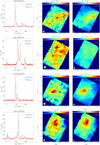 |
Fig. 2 Left column: 13CO(1–0) (black) and 13CO(2–1) (red) spectra averaged towards the full IRDC maps. The velocity ranges considered for each cloud are indicated with vertical dotted magenta lines and are reported in Table 2. Middle and left columns: integrated intensity maps of the 13CO(1–0) and 13CO(2–1) obtained over the defined velocity ranges. In both sets of panels, the beam sizes and 1 pc scale bar are indicated. |
Properties of the four IRDCs and observed maps.
Spectroscopic information for the 13CO(1–0) and (2–1) transitions.
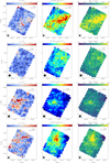 |
Fig. 3 Maps of the column-density-weighted excitation temperature (left column), 13CO column density (middle column), and 13CO-derived mass surface density (right column) obtained for the four IRDCs (the top to bottom rows show G24.94-00.15, G23.46-00.53, G24.49-00.70, and G25.16-00.28). In each panel, the black contour corresponds to the FIR-derived mass surface density of 0.1 g cm−2. |
 |
Fig. 4 CO depletion factor (left column) and corrected CO depletion factor (right column). In each panel, the white contours mark ΣFIR = 0.1 g cm−2. The beam size and 1pc scale are indicated in the bottom left and top right corner, respectively. |
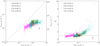 |
Fig. 5 Left: 13CO-derived mass surface density, Σ13CO, as a function of the Herschel-derived mass surface density, ΣFIR, for all clouds in our sample (different colours). The dotted line corresponds to the one-to-one line. Right: normalised CO depletion factor, |


Average values extracted for all four IRDCs.
4.3 CO depletion
In Figure 5, we show a scatter plot of Σ13CO versus ΣFIR for all the pixels in the maps of IRDCs O, V, X, and Y. The 13CO-derived mass surface densities are in the range 0.003–0.05 g cm−2. While Σ13CO increases with ΣFIR, it remains systematically lower by factors of ∼3–25, and this factor grows towards the high-Σ regime. This discrepancy between Σ13CO and ΣFIR might be evidence of CO depletion. Alternatively, other factors might cause a systematic underestimation of Σ via 13CO emission or an overestimation via FIR dust continuum emission.
One potential explanation that was also discussed by Hernandez et al. (2012) is that a strong negative excitation temperature gradient from the more diffuse to the denser regions of the clouds might cause Σ13CO to be underestimated. As shown in Figure 3, however, we observe no such trend in any of the IRDCs. In contrast, we see indications of a rise of Tex towards the denser regions.
Local fractionation of the 13CO isotope might also explain the low values of Σ13CO. Two possible mechanisms might account for this: isotope-selective photo-dissociation, and chemical fractionation. For isotope-selective photo-dissociation, however, the effect is known to be negligible for H volume densities >102 cm−3 (Szűcs et al. 2014), with this limit well below the average IRDC densities in our clouds. Chemical fractionation, on the other hand, is predicted to become effective for 12CO column densities in the range 1015–1017 cm−2. At the considered 12C/13C ratio of 51, this corresponds to 13CO column densities in the range 2 × 10¹³–2 × 1015 cm−2. Towards the four IRDCs, we estimate N13CO ≥ 1016 cm−3, and while chemical fractionation might occur to some extent, it is therefore most likely not the main cause of the low Σ13CO we obtained. Moreover, recent simulations also suggested new exchange reactions that might increase the production of 13CO for molecules produced from atomic C (Colzi et al. 2020).
Finally, the dust opacity assumptions adopted by Lim et al. (2016) might affect the ΣFIR estimates. The effects of these assumptions are already considered in the 30% uncertainty reported by the authors and can only account for a small fraction of the ΣFIR variations. In light of all this, we conclude that the relatively low values of Σ13CO are primarily due to the depletion of CO from the gas phase onto dust grains.
To quantify CO depletion, following previous studies (e.g. Caselli et al. 1999; Fontani et al. 2006; Hernandez et al. 2011; Jiménez-Serra et al. 2014), we defined the CO depletion factor as
 (7)
(7)
The corresponding CO depletion maps are shown in Figure 4. In order to take the systematic uncertainties due to the assumed CO abundance and the Herschel-derived ΣFIR into account, we re-normalised fD, so that it was ∼1 for Tdust ≥20 K, that is, the CO freeze-out temperature (Caselli et al. 1999). We note that this temperature roughly corresponds to a value of Σ ∼ 0.1 g cm−2 for all the clouds. We indicate this normalised CO depletion factor as  and show the obtained maps in Figure 4. For each cloud, the normalisation factors, β, are reported in Table 4, along with the column-density-weighted mean excitation temperatures.
Figure 4 shows that the CO depletion factor takes values fD ∼ 3–25 or  after normalisation. For an average cloud kinematic distance of 3 kpc (Table 2), the 8.5″ pixel scale in our maps corresponds to ∼0.125 pc and contains 7.4 × (Σ13CO/0.1g cm−2) M⊙. Hence, several tens of solar masses per pixel are missed when using CO observations when depletion is not taken into account.
The CO depletion values shown in Figure 4 are consistent with those reported by previous studies of IRDCs within the sample by Butler & Tan (2012). Hernandez et al. (2011) reported normalised CO depletion factors up to 5 towards IRDC G035.39-00.33 (cloud H in Butler & Tan 2012), using C18O emission. Towards the same source, Jiménez-Serra et al. (2014) obtained fD up to 12 from a non-LTE analysis of the 13CO emission. Entekhabi et al. (2022) used astrochemical models to infer the CO depletion factors towards ten massive clumps in IRDC G028.37 (cloud C in Butler & Tan 2012). For these regions, Entekhabi et al. (2022) reported fD up to 10, which is slightly higher than the values reported here. The dust temperatures in the ten clumps we studied in cloud C are colder, however, as discussed further below. Sabatini et al. (2019) reported fD ≤ 6 towards IRDC G351.77-0.51, which is similar to our  values. Our normalised CO depletion estimates are also consistent with those measured towards high-mass star-forming clumps by Feng et al. (2020) (up to 15) and Fontani et al. (2012), that is, ≤10 for a sub-sample of clumps located at distances similar to our sources.
We also investigated how the CO depletion factor varied as a function of the cloud properties of H number density and dust temperature, as shown in Figure 6. Here, we also included the fD values measured by Entekhabi et al. (2022) in IRDC G28.37 (Cloud C). The H number densities shown in Figure 6 were obtained by applying the machine-learning denoising diffusion probabilistic model described by Xu et al. (2023) to the Herschel-derived mass surface density maps. For a detailed description of the method, we refer to Xu et al. (2023). As shown in Figure 6, the CO depletion factor exhibits clear trends as a function of nH and Tdust. In particular, denser and colder regions show higher levels of CO depletion. The scatter in the relation of fD with density is relatively high, especially if the cloud C were also considered. On the other hand, the relation of CO depletion with temperature follows a monotonic relation more tightly.
The correlation between the large-scale CO depletion in IRDCs and the cloud properties was considered in previous works (e.g. Kramer et al. 1999; Fontani et al. 2011; Sabatini et al. 2019). These studies generally reported evidence of a correlation between nH and fD that is broadly consistent with our results. Only Fontani et al. (2011) observed a slight anti-correlation between the two quantities, but also suggested this might be due to beam-dilution effects. Kramer et al. (1999) and Sabatini et al. (2019) also investigated the relation between fD and Tdust for low-mass star-forming regions and IRDCs, respectively, and reported qualitatively similar trends to our results.
In the right panel of Figure 6, we show the functional form of fD(Tdust) derived by Kramer et al. (1999) (see Eq. (1)). It does not track the rapid rise of fD, which occurs at Tdust ≲ 18 K. This might reflect real differences in the molecular cloud environments between the low-mass core IC 5146 and our IRDC sample: especially the range of Σ in the low-mass core is much smaller, that is, Σ ≲ 0.1 g cm−2, than our IRDCs, where 0.1 g cm−2 ≲ Σ ≲ 0.7 g cm−2. Alternatively, as mentioned in §1, systematic uncertainties in measurement of Tdust might be at play.
In Figure 6, we also present a new functional form for  that is a better description of IRDC conditions (taking the uncertainties on
  and Tdust into account),
![Mathematical equation: ${{f'}_D} = \exp \left[ {{{{T_0}} \over {({T_{{\rm{dust}}}} - {T_1})}}} \right].$](/articles/aa/full_html/2026/01/aa57102-25/aa57102-25-eq30.png) (8)
(8)
The example curve shown in Fig. 6 has T0 = 4 K and T1 = 12 K. The validity in the temperature range is ∼15 K ≲ Tdust ≲ 30 K. The main feature of the relation is the rapid rise of the depletion factor at temperatures ≲18 K.
These results suggest overall that the dust temperature and not the density is the most important variable in controlling the CO depletion factor. In addition, the relatively small amount of scatter seen in the  relation might indicate than CO depletion has reached a near equilibrium value, that is, a balance in the rates of freeze-out and desorption, with the latter being dominated by thermal desorption and not by non-thermal (e.g. cosmic-ray induced) desorption processes. We anticipate that these results will be important constraints for astrochemical models of molecular clouds (see also Entekhabi et al. 2022) and for their chemodynamical history (e.g. Hsu et al. 2023).
 |
Fig. 6 Corrected CO depletion factors, |


5 Conclusions
We have used 13CO(1–0) and (2–1) observations to infer the levels of CO depletion towards a sample of four IRDCs. We found normalised CO depletion factors up to 10 that cannot be explained by systematic uncertainties in our analysis or chemical effects alone. We found that CO depletion generally increases with increasing cloud density, although with significant scatter. There is a tighter correlation with the dust temperature, with CO depletion rising rapidly for Tdust ≲ 18 K. To capture this behaviour, we proposed a functional form for the normalised CO depletion factor of ![Mathematical equation: ${f'_D} = A\exp \left( {{T_0}/\left[ {{T_{{\rm{dust}}}} - {T_1}} \right]} \right)$](/articles/aa/full_html/2026/01/aa57102-25/aa57102-25-eq32.png) with values of the coefficients T0 ≃ 4 K and T1 ≃ 12 K. These results indicate overall that the dust temperature is the most important variable in controlling the CO depletion factor. The relatively small amount of scatter might indicate that the level of gas-phase CO has reached near equilibrium values, with thermal desorption playing a dominant role in balancing freeze-out. These results provide important constraints for astrochemical models and for the chemodynamical history of gas during the early stages of star formation.
with values of the coefficients T0 ≃ 4 K and T1 ≃ 12 K. These results indicate overall that the dust temperature is the most important variable in controlling the CO depletion factor. The relatively small amount of scatter might indicate that the level of gas-phase CO has reached near equilibrium values, with thermal desorption playing a dominant role in balancing freeze-out. These results provide important constraints for astrochemical models and for the chemodynamical history of gas during the early stages of star formation.
Acknowledgements
G.C. acknowledges support from the Swedish Research Council (VR Grant; Project: 2021-05589). J.C.T. acknowledges support from ERC project 788829 (MSTAR). I.J.-S. acknowledges funding from grant PID2022-136814NB-I00 funded by the Spanish Ministry of Science, Innovation and Universities/State Agency of Research MICIU/AEI/10.13039/501100011033 and by “ERDF/EU”. J.D.H. gratefully acknowledges financial support from the Royal Society (University Research Fellowship; URF/R1/221620). S.V. acknowledges partial funding from the European Research Council (ERC) Advanced Grant MOPPEX 833460. This work is based on observations carried out under project number 013-20 with the IRAM 30m telescope. IRAM is supported by INSU/CNRS (France), MPG (Germany) and IGN (Spain). This publication makes use of data from FUGIN, FOREST Unbiased Galactic plane Imaging survey with the Nobeyama 45-m telescope, a legacy project in the Nobeyama 45-m radio telescope.
References
- Butler, M. J., & Tan, J. C. 2009, ApJ, 696, 484 [NASA ADS] [CrossRef] [Google Scholar]
- Butler, M. J., & Tan, J. C. 2012, ApJ, 754, 5 [Google Scholar]
- Caselli, P., Walmsley, C. M., Tafalla, M., Dore, L., & Myers, P. C. 1999, ApJ, 523, L165 [Google Scholar]
- Caselli, P., Benson, P. J., Myers, P. C., & Tafalla, M. 2002, ApJ, 572, 238 [Google Scholar]
- Caselli, P., Vastel, C., Ceccarelli, C., et al. 2008, A&A, 492, 703 [NASA ADS] [CrossRef] [EDP Sciences] [Google Scholar]
- Christie, H., Viti, S., Yates, J., et al. 2012, MNRAS, 422, 968 [NASA ADS] [CrossRef] [Google Scholar]
- Churchwell, E., Babler, B. L., Meade, M. R., et al. 2009, PASP, 121, 213 [Google Scholar]
- Clarke, S. D., Makeev, V. A., Sánchez-Monge, Á., et al. 2024, MNRAS, 528, 1555 [Google Scholar]
- Colzi, L., Sipilä, O., Roueff, E., Caselli, P., & Fontani, F. 2020, A&A, 640, A51 [NASA ADS] [CrossRef] [EDP Sciences] [Google Scholar]
- Crapsi, A., Caselli, P., Walmsley, C. M., et al. 2005, ApJ, 619, 379 [Google Scholar]
- Dalgarno, A., & Lepp, S. 1984, ApJ, 287, L47 [NASA ADS] [CrossRef] [Google Scholar]
- Egan, M. P., Shipman, R. F., Price, S. D., et al. 1998, ApJ, 494, L199 [Google Scholar]
- Entekhabi, N., Tan, J. C., Cosentino, G., et al. 2022, A&A, 662, A39 [NASA ADS] [CrossRef] [EDP Sciences] [Google Scholar]
- Feng, S., Li, D., Caselli, P., et al. 2020, ApJ, 901, 145 [Google Scholar]
- Fontani, F., Caselli, P., Crapsi, A., et al. 2006, A&A, 460, 709 [NASA ADS] [CrossRef] [EDP Sciences] [Google Scholar]
- Fontani, F., Palau, A., Caselli, P., et al. 2011, A&A, 529, L7 [NASA ADS] [CrossRef] [EDP Sciences] [Google Scholar]
- Fontani, F., Giannetti, A., Beltrán, M. T., et al. 2012, MNRAS, 423, 2342 [NASA ADS] [CrossRef] [Google Scholar]
- Ford, A. B., & Shirley, Y. L. 2011, ApJ, 728, 144 [NASA ADS] [CrossRef] [Google Scholar]
- Fortune-Bashee, X., Sun, J., & Tan, J. C. 2024, ApJ, 977, L6 [Google Scholar]
- Foster, J. B., Arce, H. G., Kassis, M., et al. 2014, ApJ, 791, 108 [NASA ADS] [CrossRef] [Google Scholar]
- Frerking, M. A., Langer, W. D., & Wilson, R. W. 1982, ApJ, 262, 590 [Google Scholar]
- Gong, Y., Belloche, A., Du, F. J., et al. 2021, A&A, 646, A170 [NASA ADS] [CrossRef] [EDP Sciences] [Google Scholar]
- Herbst, E., & van Dishoeck, E. F. 2009, ARA&A, 47, 427 [Google Scholar]
- Hernandez, A. K., & Tan, J. C. 2015, ApJ, 809, 154 [NASA ADS] [CrossRef] [Google Scholar]
- Hernandez, A. K., Tan, J. C., Caselli, P., et al. 2011, ApJ, 738, 11 [NASA ADS] [CrossRef] [Google Scholar]
- Hernandez, A. K., Tan, J. C., Kainulainen, J., et al. 2012, ApJ, 756, L13 [NASA ADS] [CrossRef] [Google Scholar]
- Hirata, Y., Kawamura, A., Nishimura, A., et al. 2024, PASJ, 76, 65 [Google Scholar]
- Hsu, C.-J., Tan, J. C., Holdship, J., et al. 2023, arXiv e-prints [arXiv:2308.11803] [Google Scholar]
- Inutsuka, S.-i., Inoue, T., Iwasaki, K., & Hosokawa, T. 2015, A&A, 580, A49 [NASA ADS] [CrossRef] [EDP Sciences] [Google Scholar]
- Jiménez-Serra, I., Caselli, P., Fontani, F., et al. 2014, MNRAS, 439, 1996 [Google Scholar]
- Kainulainen, J., & Tan, J. C. 2013, A&A, 549, A53 [NASA ADS] [CrossRef] [EDP Sciences] [Google Scholar]
- Kong, S., Caselli, P., Tan, J. C., Wakelam, V., & Sipilä, O. 2015, ApJ, 804, 98 [NASA ADS] [CrossRef] [Google Scholar]
- Kong, S., Tan, J. C., Caselli, P., et al. 2017, ApJ, 834, 193 [NASA ADS] [CrossRef] [Google Scholar]
- Kramer, C., Alves, J., Lada, C. J., et al. 1999, A&A, 342, 257 [NASA ADS] [Google Scholar]
- Li, Q., Tan, J. C., Christie, D., Bisbas, T. G., & Wu, B. 2018, PASJ, 70, S56 [NASA ADS] [Google Scholar]
- Lim, W., Tan, J. C., Kainulainen, J., Ma, B., & Butler, M. J. 2016, ApJ, 829, L19 [NASA ADS] [CrossRef] [Google Scholar]
- Milam, S. N., Savage, C., Brewster, M. A., Ziurys, L. M., & Wyckoff, S. 2005, ApJ, 634, 1126 [Google Scholar]
- Morii, K., Sanhueza, P., Nakamura, F., et al. 2021, ApJ, 923, 147 [NASA ADS] [CrossRef] [Google Scholar]
- Moser, E., Liu, M., Tan, J. C., et al. 2020, ApJ, 897, 136 [NASA ADS] [CrossRef] [Google Scholar]
- Perault, M., Omont, A., Simon, G., et al. 1996, A&A, 315, L165 [NASA ADS] [Google Scholar]
- Peretto, N., Lenfestey, C., Fuller, G. A., et al. 2016, A&A, 590, A72 [NASA ADS] [CrossRef] [EDP Sciences] [Google Scholar]
- Pillai, T., Wyrowski, F., Carey, S. J., & Menten, K. M. 2006, A&A, 450, 569 [NASA ADS] [CrossRef] [EDP Sciences] [Google Scholar]
- Pillai, T., Kauffmann, J., Zhang, Q., et al. 2019, A&A, 622, A54 [NASA ADS] [CrossRef] [EDP Sciences] [Google Scholar]
- Rathborne, J. M., Jackson, J. M., & Simon, R. 2006, ApJ, 641, 389 [Google Scholar]
- Redaelli, E., Bovino, S., Giannetti, A., et al. 2021, A&A, 650, A202 [NASA ADS] [CrossRef] [EDP Sciences] [Google Scholar]
- Redaelli, E., Bovino, S., Sanhueza, P., et al. 2022, ApJ, 936, 169 [NASA ADS] [CrossRef] [Google Scholar]
- Retes-Romero, R., Mayya, Y. D., Luna, A., & Carrasco, L. 2020, ApJ, 897, 53 [NASA ADS] [CrossRef] [Google Scholar]
- Sabatini, G., Giannetti, A., Bovino, S., et al. 2019, MNRAS, 490, 4489 [Google Scholar]
- Sabatini, G., Bovino, S., Giannetti, A., et al. 2020, A&A, 644, A34 [EDP Sciences] [Google Scholar]
- Sabatini, G., Bovino, S., Sanhueza, P., et al. 2022, ApJ, 936, 80 [NASA ADS] [CrossRef] [Google Scholar]
- Sabatini, G., Bovino, S., Redaelli, E., et al. 2024, A&A, 692, A265 [NASA ADS] [CrossRef] [EDP Sciences] [Google Scholar]
- Simon, R., Rathborne, J. M., Shah, R. Y., Jackson, J. M., & Chambers, E. T. 2006, ApJ, 653, 1325 [NASA ADS] [CrossRef] [Google Scholar]
- Socci, A., Caselli, P., Sipilä, O., et al. 2024, A&A, 687, A70 [NASA ADS] [CrossRef] [EDP Sciences] [Google Scholar]
- Suwannajak, C., Tan, J. C., & Leroy, A. K. 2014, ApJ, 787, 68 [Google Scholar]
- Szűcs, L., Glover, S. C. O., & Klessen, R. S. 2014, MNRAS, 445, 4055 [CrossRef] [Google Scholar]
- Tan, J. C. 2000, ApJ, 536, 173 [NASA ADS] [CrossRef] [Google Scholar]
- Tan, J. C. 2010, ApJ, 710, L88 [Google Scholar]
- Tan, J. C., Kong, S., Butler, M. J., Caselli, P., & Fontani, F. 2013, ApJ, 779, 96 [Google Scholar]
- Tan, J. C., Beltrán, M. T., Caselli, P., et al. 2014, in Protostars and Planets VI, eds. H. Beuther, R. S. Klessen, C. P. Dullemond, & T. Henning, 149 [Google Scholar]
- Tasker, E. J., & Tan, J. C. 2009, ApJ, 700, 358 [NASA ADS] [CrossRef] [Google Scholar]
- Umemoto, T., Minamidani, T., Kuno, N., et al. 2017, PASJ, 69, 78 [Google Scholar]
- Vázquez-Semadeni, E., Palau, A., Ballesteros-Paredes, J., Gómez, G. C., & Zamora-Avilés, M. 2019, MNRAS, 490, 3061 [Google Scholar]
- Whittet, D. C. B., Goldsmith, P. F., & Pineda, J. L. 2010, ApJ, 720, 259 [NASA ADS] [CrossRef] [Google Scholar]
- Wu, B., Van Loo, S., Tan, J. C., & Bruderer, S. 2015, ApJ, 811, 56 [NASA ADS] [CrossRef] [Google Scholar]
- Wu, B., Tan, J. C., Nakamura, F., et al. 2017, ApJ, 835, 137 [NASA ADS] [CrossRef] [Google Scholar]
- Xu, D., Tan, J. C., Hsu, C.-J., & Zhu, Y. 2023, ApJ, 950, 146 [Google Scholar]
- Yang, B., Stancil, P. C., Balakrishnan, N., & Forrey, R. C. 2010, ApJS, 188, 581 [Google Scholar]
- Yu, H., Wang, J., & Tan, J. C. 2020, ApJ, 905, 78 [Google Scholar]
- Zhang, Q., Wang, Y., Pillai, T., & Rathborne, J. 2009, ApJ, 696, 268 [Google Scholar]
All Tables
All Figures
|
Fig. 1 Spitzer 8 µm images (left column), Herschel-derived mass surface density maps (Σ; middle column) and dust temperature (Tdust; right column) for the four IRDCs. In the middle and right panels, the Σ=0.1 g cm−2 black contours highlight the shape of each cloud. The beam size (bottom left) and 1 pc scale bar (top right) are also indicated. |
| In the text | |
|
Fig. 2 Left column: 13CO(1–0) (black) and 13CO(2–1) (red) spectra averaged towards the full IRDC maps. The velocity ranges considered for each cloud are indicated with vertical dotted magenta lines and are reported in Table 2. Middle and left columns: integrated intensity maps of the 13CO(1–0) and 13CO(2–1) obtained over the defined velocity ranges. In both sets of panels, the beam sizes and 1 pc scale bar are indicated. |
| In the text | |
|
Fig. 3 Maps of the column-density-weighted excitation temperature (left column), 13CO column density (middle column), and 13CO-derived mass surface density (right column) obtained for the four IRDCs (the top to bottom rows show G24.94-00.15, G23.46-00.53, G24.49-00.70, and G25.16-00.28). In each panel, the black contour corresponds to the FIR-derived mass surface density of 0.1 g cm−2. |
| In the text | |
|
Fig. 4 CO depletion factor (left column) and corrected CO depletion factor (right column). In each panel, the white contours mark ΣFIR = 0.1 g cm−2. The beam size and 1pc scale are indicated in the bottom left and top right corner, respectively. |
| In the text | |
|
Fig. 5 Left: 13CO-derived mass surface density, Σ13CO, as a function of the Herschel-derived mass surface density, ΣFIR, for all clouds in our sample (different colours). The dotted line corresponds to the one-to-one line. Right: normalised CO depletion factor, |
| In the text | |
|
Fig. 6 Corrected CO depletion factors, |
| In the text | |
Current usage metrics show cumulative count of Article Views (full-text article views including HTML views, PDF and ePub downloads, according to the available data) and Abstracts Views on Vision4Press platform.
Data correspond to usage on the plateform after 2015. The current usage metrics is available 48-96 hours after online publication and is updated daily on week days.
Initial download of the metrics may take a while.