| Issue |
A&A
Volume 699, July 2025
|
|
|---|---|---|
| Article Number | A268 | |
| Number of page(s) | 8 | |
| Section | Astrophysical processes | |
| DOI | https://doi.org/10.1051/0004-6361/202555202 | |
| Published online | 11 July 2025 | |
Fine-structure excitation of C2O by He: Rate coefficients and astrophysical modeling
1
Departamento de Química Física, University of Salamanca, Plaza Caídos s/n, E-37008 Salamanca, Spain
2
Univ. Rennes, CNRS, IPR (Institut de Physique de Rennes) – UMR 6251, 35000 Rennes, France
3
Physics Department, Khalifa University, Abu-Dhabi, United Arab Emirates
4
Nantes Université, CNRS, CEISAM, UMR 6230, F-44000 Nantes, France
⋆ Corresponding authors: This email address is being protected from spambots. You need JavaScript enabled to view it.
, This email address is being protected from spambots. You need JavaScript enabled to view it.
Received:
18
April
2025
Accepted:
16
May
2025
Abstract
Context. C2O molecules are very good probes of oxygen chemistry in interstellar molecular clouds. The accurate derivation of their abundance requires non-local thermodynamic equilibrium (LTE) modeling of their emission spectra.
Aims. This study aims to provide highly accurate fine-structure resolved excitation rate coefficients of C2O induced by collisions with He, enabling the improvement of the modeling of C2O emission spectra in (cold) molecular clouds.
Methods. A new potential energy surface for the C2O–He system was calculated using the spin-restricted coupled-cluster method together with a complete atomic basis set extrapolation. Quantum scattering calculations were performed using the exact close-coupling approach, explicitly accounting for the fine structure of C2O. Excitation calculations using a radiative transfer model were conducted in order to interpret observations of C2O in TMC-1.
Results. Rate coefficients for transitions up to the rotational state N = 20 and temperatures up to 70 K were obtained. The analysis of the excitation calculations revealed non-LTE effects of C2O emission lines at typical densities of TMC-1 (n(H2)∼104 cm−3), reflecting a balance between collisional excitation and radiative relaxation. These effects significantly influence the derived physical conditions. The column density of C2O in TMC-1 was estimated to be NC2O ≈ 9 · 1011 cm−2. This refined value, derived using the newly calculated rate coefficients, highlights the limitations of previous LTE-based estimates and underscores the importance of non-LTE modeling.
Conclusions. The new accurate collisional data enable a more confident modeling of C2O excitation in interstellar clouds and improve the interpretation of C2O emission spectra in molecular clouds, highlighting again the necessity of having accurate molecular data in astrochemical studies.
Key words: astrochemistry / radiative transfer / scattering / ISM: abundances / ISM: molecules
© The Authors 2025
 Open Access article, published by EDP Sciences, under the terms of the Creative Commons Attribution License (https://creativecommons.org/licenses/by/4.0), which permits unrestricted use, distribution, and reproduction in any medium, provided the original work is properly cited.
This article is published in open access under the Subscribe to Open model. This email address is being protected from spambots. You need JavaScript enabled to view it. to support open access publication.
1. Introduction
Oxygen-bearing carbon chains (CnO), such as C2O, are essential probes of oxygen chemistry in interstellar molecular clouds. They provide critical insights into the role of oxygen chemistry in astrophysical processes, such as the synthesis of complex molecules and the thermal regulation of interstellar clouds (Agúndez & Wakelam 2013).
C2O was first detected in TMC-1 by Ohishi et al. (1991). Urso et al. (2019) reported the first detection of the C2O in the L1544 prestellar core and in the Elias 18 protostar, revealing the presence of C2O in other molecular clouds than TMC-1. More recently, C2O was again observed by Cernicharo et al. (2020, 2021) in TMC-1, further confirming it is an important constituent of molecular clouds. In particular, Cernicharo et al. (2020) reported the detection of C2O along with other oxygen-bearing carbon chains, using observations from the Yebes 40m and IRAM 30m telescopes. They also provided rotational temperatures and column densities for the detected species derived from spectral line analysis. Subsequently, Cernicharo et al. (2021) enhanced the observational data by using the Q-band Ultrasensitive Inspection Journey to the Obscure TMC-1 Environment (QUIJOTE) line survey, providing a more accurate determination of column densities for C2O and related species (HCnO and CnO).
The lack of accurate collisional rate coefficients for C2O under specific physical conditions of (cold) molecular clouds is a significant limitation for the accurate modeling of the C2O observations. Indeed, in TMC-1 and similar molecular clouds, the low densities prevent local thermodynamic equilibrium (LTE) from being achieved. As a result, modeling the observational spectra requires excitation calculations using radiative transfer models that include both radiative and collisional processes. To overcome this limitation, Cernicharo et al. (2021) estimated rate coefficients for C2O using collisional data for the OCS(1Σ+) molecule and employing the infinite-order-sudden (IOS) approximation to model collisional transitions between fine-structure levels of C2O. Indeed, we remind the reader that C2O is a 3Σ− electronic state molecule exhibiting a fine structure due to the coupling between the rotational levels, N, and the electronic spin, S. Although this approach allows for a preliminary analysis, it does not provide the required level of accuracy, as has previously been shown for systems such as C2S (Palluet & Lique 2023).
The aim of this paper is to overcome this limitation and to provide collisional rate coefficients for the C2O molecules that are essential for understanding the excitation processes occurring in interstellar molecular clouds. Projectiles like H2 and He play a crucial role in the excitation processes that take place in such an environment. Scattering calculations involving H2 are challenging because of its internal rotational structure. As a result, He is often used as a proxy for para-H2 (the main constituent of cold molecular clouds such as TMC-1) due to their similar electronic structures and the fact that each possesses two valence electrons and exhibits spherical symmetry (Roueff & Lique 2013).
Recently, Khadri et al. (2022) performed the first scattering calculations for the C2O−He collisional system. Their work included the calculation of the first potential energy surface (PES) for the C2O−He interacting system as well as scattering data, such as cross sections and rate coefficients, obtained for rotational levels up to N = 10 (e.g., neglecting the fine-structure splitting). Additionally, they employed the recoupling technique proposed by Corey et al. (1986) to account for the fine-structure of C2O and to provide fine-structure resolved collisional rate coefficients. While the PES developed by Khadri et al. (2022) is accurate, their scattering calculations exhibit some limitations. Specifically, the recoupling approximation used to derive fine-structure cross sections and rate coefficients, while computationally efficient, is moderately accurate for systems with significant fine-structure splittings, particularly at low collision energies and for transitions involving low rotational levels (Orlikowski 1985; Lique et al. 2005). Furthermore, their study included a limited number of rotational levels (N) (up to N = 10) at kinetic temperatures up to T = 80 K, whereas it has been established that higher rotational levels could be significantly populated at such temperatures.
To the best of our knowledge, the study by Khadri et al. (2022) is the only investigation of the C2O−He collisional system to date. Hence, in this paper, we update the previous study and present a new C2O−He PES calculated using a single-reference coupled-cluster method that is used after to study the fine-structure (de-)excitations of C2O induced by collisions with He. The excitation cross sections of C2O induced by He were computed using the close-coupling (CC) quantum approach, explicitly accounting for the C2O fine structure. Then, fine-structure resolved rate coefficients were obtained for temperatures up to 70 K and for fine-structure levels up to N = 20. As a first astrophysical application, we used these refined data to improve the interpretation of C2O observations in TMC-1. To achieve this, the new rate coefficients were used in radiative transfer models performed with the RADEX code (van der Tak et al. 2007) and the predictions were compared to the first C2O detection in TMC-1 in order to derive the column density of the molecule.
This paper is structured as follows. Section 2 contains the computational methods used to obtain the PES and a description of the methods used to calculate the scattering data for the C2O−He system. In Section 3.1 we present the new calculated PES. In Section 3.2 we provide the cross sections and rate coefficients for C2O−He collisional system. In Section 4 the results and interpretations of the astrophysical modeling are shown. Section 5 contains the final concluding remarks.
2. Methods
2.1. Potential energy surface
The interaction potential of the C2O−He system was calculated using the spin restricted coupled-cluster single double and perturbative triple excitations ab initio method [RCCSD(T)] (Knowles et al. 1993, 2000). The basis set considered for these electronic structure calculations were the aug-cc-pVXZ (Dunning 1989), with X=T,Q,5, in order to perform a complete basis set (CBS) extrapolation. All the calculations were carried out with the MOLPRO 2020 suite of programs (Werner et al. 2020). The coupled-cluster method together with the CBS extrapolation is widely recognized as the gold standard for describing weak van der Waals interactions such as the ones occurring in the C2O−He complex. Hence, we expect the new C2O−He PES to be highly accurate.
The interaction potential of C2O with He was computed using the Jacobi coordinates (R,θ), where R is the distance between the He atom and the center of mass of the C2O molecule, and θ is the angle between the Jacobi vector, R, and the internuclear axis of the C2O molecule (see Figure 1). The C2O(3Σ−) molecule was treated as a linear rigid rotor with equilibrium bond lengths taken from Ohshima et al. (1995). We have considered 46 different values of R between 4.5 a0 and 30 a0, and 26 values for θ. To effectively describe the most significant interaction parts, we used a nonuniform step for R distances. For the angular component, we used a 5° step for θ in the θ = 65−125° range and a 10° step for the θ = 0−60° and θ = 130−180° intervals.
 |
Fig. 1. Definition of the C2O−He Jacobi coordinate system (R,θ). The center of mass (COM) is indicated in yellow. |
The extrapolation to the CBS limit was performed using the extrapolation scheme of Peterson et al. (1994):
 (1)
(1)
where EX is the interaction energy obtained with the aug-cc-pVXZ basis set, and A and B are the parameters to be adjusted for all geometries of the C2O−He complex. This system of equations lead to ECBS, which is the interaction energy extrapolated to the complet basis set limit. Additionally, we corrected the BSSE (basis set superposition error) at each (R,θ) geometry using the Boys and Bernardi counterpoise procedure (Boys & Bernardi 1970):
 (2)
(2)
where V(R,θ) is the interaction potential, and  ,
,  , and EHe(R,θ) are the total electronic energies of the complex, and the C2O and He monomers, respectively, computed using the full basis set of the complex.
2.2. Fitting procedure
The construction of the analytical PES was performed using the recently developed Radial Angular Network with Gradual Expansion (RANGE) method (Bop & Lique 2024), specifically developed for systems with high angular anisotropy, such as carbon-chain molecules. The use of RANGE makes it possible to obtain an accurate fit of the PES, while limiting the number of angular functions, which is important for speeding up the scattering calculations.
The RANGE procedure starts by gradually expanding the angular grid from the T-shaped geometry (90°) to the collinear configurations (0° and 180°), but it explicitly avoids extremely repulsive potential values in these regions. In particular, the method avoids small (θ near to 0°) and large (θ near to 180°) values of θ, where the interaction potential becomes highly repulsive. The angular expansion is done for each R distance. Considering this grid, the ab initio points were fit via the usual Legendre polynomials Pl(cos(θ)):
 (3)
(3)
where lmax is the maximum value of angular functions. The lmax depends on the distance and corresponds to the number of value of θ that has been considered for a given R. In this work, lmax was set to 17.
2.3. Fine structure for the C2O(3Σ−) molecule
The C2O molecule in its ground electronic state, 3Σ− state, is an open-shell molecule. As a result, the electronic spin (S) of the molecule couples with its rotational angular momentum (N), leading to the splitting of the rotational energy levels into fine-structure levels. The rotational energy levels are then described using the intermediate coupling scheme (Lique et al. 2005), where the total angular momentum (j) is determined by the coupling between both momenta, N and S, as:
 (4)
(4)
For a 3Σ− electronic state molecule, where S = 1, the rotational wave function, |Fi jm〉, is expressed as
 (5)
(5)
where |N,Sjm〉 represents the wave function in a pure Hund’s case (b) (Corey et al. 1986) and α is the mixing angle obtained from diagonalization of the molecular Hamiltonian. When α→0, the energy levels can be described by the pure Hund’s case (b) limit and the fine rotational levels, Fi, will correspond to
 (6)
(6)
Hereafter, we use the astrophysical notation, Nj, corresponding to the pure Hund’s case (b). However, it is important to note that all scattering calculations were performed using the intermediate coupling scheme. The fine-structure levels for the C2O(3Σ−) were computed with the spectroscopic constants reported by Abusara et al. (2003) and are presented in Table 1. For N<13, for a given fine-structure manifold, the F3 level lies below F1, while for N≥13, the order is reversed. The F2 level is always the highest energy level of the manifold, regardless of the value of N.
Fine-structure energy levels of the C2O(3Σ−) diradical.
2.4. Quantum dynamics
The determination of the excitation cross section ( ) of C2O(3Σ−) induced by He was performed using the standard CC (Arthurs & Dalgarno 1960; Lique et al. 2005) approach. All the scattering calculations were performed with the MOLSCAT (Hutson & Le Sueur 2019) computer code. The propagator of (Manolopoulos 1986) was used in all calculations. We aimed to determine excitation cross sections between the first N = 20 rotational levels of C2O for collision energies up to at least 300 cm−1. We performed convergence tests to achieve an accuracy of the cross sections of ≃1−2%. For total energies between 300 and 500 cm−1, Rmin was set to 4.2 a0, while for all other total energies, Rmin = 4.5 a0 was used. For all total energies, Rmax was set to at least 50 a0. The number of energy levels included in the calculations (defined by Nmax) and the step of propagation of the wave function (which depends on the STEPS parameter) depend on the total energy and are reported in Table 2. The MOLSCAT code automatically set the total angular momentum (Jmax) required for convergence. The total energy spacing (in cm−1) for cross section calculations was set at 0.2 between 1−100 cm−1, 0.5 between 100 and 300 cm−1, and 2 between 300 and 500 cm−1.
Parameters used in the MOLSCAT scattering calculations as a function of the total energy (E).
The rate coefficients were obtained by averaging the cross sections over a Maxwell-Boltzmann distribution of the relative kinetic energy values ( ) between partners:
 (7)
(7)
where E is the total energy and  is the energy of the fine-structure level (Nj). The reduced mass, μ, for the C2O−He system is 3.6385 amu. The cross section calculations of up to at least Ek = 300 cm−1 allow one to derive rate coefficients up to 70 K.
3. Results
3.1. Potential energy surface
We present in Figure 2 the contour plot of the C2O−He PES. The global minimum is at V=−41.09 cm−1 for R = 6.20 a0 and in a nearly T-shaped configuration (θ = 81°). The PES exhibits a strong angular anisotropy. The anisotropy is even stronger when the He atom approaches the terminal carbon atom (θ = 100−180°). In comparison, the PES calculated by Khadri et al. (2022) using the explicitly correlated variant of the RCCSD(T) approach and the aug-cc-pVTZ atomic basis predicts the global minimum with a well depth of −42.376 cm−1 at R = 6.20 a0 and θ = 78°. Their minimum is very similar to the one of the new PES, both in terms of well depth and equilibrium distance. The small difference could easily be attributed to differences in the computational methods and the fitting procedures employed. However, we do not expect these differences in the two PESs to induce significant differences in the scattering calculations.
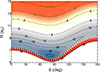 |
Fig. 2. Potential energy contours for the C2O−He system. The energy is in cm−1 and the zero is set at infinite R. |
3.2. Inelastic cross sections and rate coefficients
We computed the integral cross sections and rate coefficients for rotational (de-)excitation of C2O induced by collisions with He using the methodologies described in previous sections. In Figure 3, we present the collisional energy dependence of the cross sections and the temperature dependence of the rate coefficients for several fine-rotational transitions.
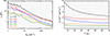 |
Fig. 3. De-excitation cross-sections (left) and rates coefficients (right) for ΔN=Δj transitions. |
The left panel of Figure 3 shows the calculated de-excitation cross sections for several ΔN=Δj transitions with the same final state, the ground fine-structure level,  . As was expected, the cross sections decrease with increasing kinetic energy, reflecting a reduced probability of an effective interaction between C2O and He at higher relative energies. At low collision energies (Ek<20−30 cm−1) some oscillations are observed in the cross sections. They can be attributed to the presence of quantum resonance effects due to bound and quasi-bound states in the C2O−He interaction potential.
The right panel of Figure 3 shows the temperature dependence of the corresponding rate coefficients. At higher temperatures, the rate coefficients are weakly dependent on the temperature, which is characteristic of collisional processes dominated by attractive interactions. The 12→01 transition presents the highest rate coefficients. This trend is directly related to their larger cross sections at low kinetic energies. Consequently, the propensity in favor of ΔN=Δj = 1 transitions, already observed in Khadri et al. (2022), is also seen in our results, showing that these transitions are faster than the others in the temperature range considered in this work.
In order to have a further look at the propensity rules, Figure 4 presents the C2O–He de-excitation rate coefficients at 10 K from Nj = 56, 55, and 54 to all possible final states. This plot highlights a clear propensity rule in favor of ΔN=Δj transitions explained by the fact that ΔN=Δj transitions do not involve a reorientation of the electronic spin projection during the collisional process. In contrast, transitions with ΔN≠Δj, that require a reorientation of the electronic spin projection, are much slower. Such a propensity rules was previously observed in other 3Σ collisional systems, such as NH(3Σ−)−He (Tobola et al. 2011), SO(3Σ−)−He (Lique et al. 2005), SO(3Σ−)−H2 (Lique et al. 2007), OH+(3Σ−)−He (González-Sánchez et al. 2007a), NH(3Σ−)−Rb/Cs (Tacconi et al. 2007), and Li2(3Σ+)−He (González-Sánchez et al. 2007b).
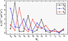 |
Fig. 4. Rate coefficients for de-excitation transitions starting from the 56, 55, and 54 levels at 10 K. |
3.3. Comparison with previous data
The only theoretical study on the excitation of C2O available to date is that of Khadri et al. (2022). We compare our newly calculated rate coefficients to their data. Table 3 presents a comparison of the two sets of rate coefficients for ΔN = 1,2,3 transitions, considering both Δj=ΔN and Δj≠ΔN transitions at 10 and 50 K. While some differences could be expected due to methodological differences, the discrepancies observed between the two datasets are much larger than what could have been anticipated.
Comparison of rate coefficients at 10 and 50 K.
These discrepancies could be due to the use of different PESs and different scattering methods to consider the fine structure of C2O. As was previously discussed, the two PES are qualitatively and quantitatively similar, so we do not expect that they can explain more than 5 to 10% of difference for the dominant transitions. At the opposite end, the recoupling approach (Corey et al. 1986) used by Khadri et al. (2022) to derive fine-structure-resolved rate coefficients is known to introduce inaccuracies (Orlikowski 1985) for systems with significant fine-structure splittings at low energies. However, the inaccuracies are on the order of 20−30% compared to an exact close coupling approach. Therefore, the deviations between the two sets of data do not seem to simply originate from the different methodological approaches used. Given the magnitude of the differences, we contacted the authors of Khadri et al. (2022) to clarify the origin of the discrepancies. Following a thorough review of their calculations, they acknowledged the presence of an error in their reported rate coefficients. Therefore, the new rate coefficients presented in this work should be considered as a more accurate reference for modeling the collisional excitation of C2O in astrophysical environments.
4. Astrophysical applications
In order to estimate the impact of the new collisional data on the astrophysical modeling, we performed excitation calculations, determined the brightness temperatures of emission lines, and compared them to observational data in TMC-1. Radiative transfer calculations for the C2O molecule were performed using the RADEX code (van der Tak et al. 2007). The kinetic temperature was fixed at Tkin = 10 K, which corresponds to the typical temperature in cold molecular clouds such as TMC-1. The background radiation temperature was set at TCMB = 2.73 K. Einstein coefficients for the radiative transitions were taken from the CDMS database (Müller et al. 2001, 2005). We included the state-to-state collisional rate coefficients of C2O−He obtained in this work. These coefficients were scaled to approximate collisions with H2 using the following relation (Lique et al. 2008):
 (8)
(8)
where μX represents the reduced mass of the colliding system, X. Such an approximation has been shown to be reasonable for relatively heavy targets with a weak to moderate dipole moment such as C2O (Roueff & Lique 2013) and usually preserves the correct propensity rules.
Figure 5 shows the variation in the excitation temperature (Tex) as a function of the H2 density ( ) for several observed transitions of the C2O molecule. Each panel corresponds to a specific transition. The calculations were performed for a column density of
  cm−2. As was expected, the excitation temperatures tend to be equal to the adopted value of the background radiation field (2.73 K) at very low volume densities of molecular hydrogen. The excitation temperatures rise to higher values as collisional excitation becomes more important. At volume densities above a critical value, the excitation temperature approaches the kinetic temperature, at which point the LTE approximation may be used. For C2O lines, the critical density lies at
  cm−3.
cm−3.
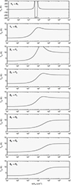 |
Fig. 5. Excitation temperature as a function of n(H2) for the transitions detected by Ohishi et al. (1991) and Cernicharo et al. (2021) at |

It is interesting to note that the upper panels (low-energy transitions) exhibit a pronounced suprathermal behavior at intermediate densities, particularly around  cm−3, the typical density in cold molecular clouds. In fact, for the lowest-energy transition (12→01), a maser effect where population inversion occurs is even observed. The opacities of these lines are low (τ<1) so that we do not expect very strong line intensities for these transitions. In contrast, the lower panels (high-energy transitions) display smoother curves dominated by subthermal behavior around
  cm−3. These results demonstrate the relevance of non-LTE effects in the excitation of C2O for
  cm−3.
cm−3.
We were then interested in reanalyzing the observations of Ohishi et al. (1991) in order to see the impact of non-LTE models on the determination of C2O column density in TMC-1. Figure 6 shows the brightness temperature (Tb in K) dependence with de H2 density and the C2O column density for the 12→01 and 23→12 transitions, the two transitions detected by Ohishi et al. (1991). We used a line width of 0.32 km s−1, in agreement with the C2O observations reported by Ohishi et al. (1991). We remind the reader that the kinetic temperature was fixed at 10 K. The dashed black isocontours in Figure 6 correspond to the observed data (33 mK for 12→01 and 50 mK for 23→12).
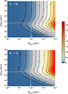 |
Fig. 6. Dependence of the 12→01 (top) and 23→12 (bottom) transition intensities (K) on column density (x axis) and n(H2) (y axis). With dashed black lines, we reproduce the isocurves of the intensities observed by Ohishi et al. (1991), and with dashed white lines the estimated column density ( |

By using the ratio of the observed brightness temperature of the two lines (Tb(12→01)/Tb(23→12) = 0.66), we can constrain the H2 density that would be able to reproduce the observations (see Figure 7). This density is around  cm−3. Although the estimated H2 density is slightly lower than the commonly reported value for TMC-1 (
 cm−3) (Fuente et al. 2019), this value is reasonable.
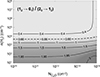 |
Fig. 7. Dependence of the intensity ratio (12→01)/(23→12) on column density (x axis) and n(H2) (y axis). The isocurve corresponding to the intensity ratio observed by Ohishi et al. (1991) is shown with dashed black lines. |
Hence, using a H2 density of approximately 7·103 cm−3, the observed line intensities point to a C2O column density of  cm−2, as is indicated by the arrows in Figure 6. Adopting the commonly reported H2 density of
  cm−3 for TMC-1 would slightly increase the derived C2O column density by 10−20%. Ohishi et al. (1991) obtained a column density of
  cm−2, approximately 1.5 times lower than our estimate. Their calculations were based on a simplified LTE model, which does not incorporate collisional rate coefficients. Such an approach often leads to the overestimation of the populations at higher-energy levels, which lead to a lower column density to reproduce the observed line intensities. This discrepancy arises because LTE models assume that the population of molecular energy levels is solely driven by the local kinetic temperature, and that collisional processes dominate over radiative ones. In environments such as TMC-1, where the gas density is relatively low, the critical densities for many transitions are not reached.
More recently, Cernicharo et al. (2021) used a non-LTE models and rate coefficients derived from the analogous OCS(1Σ+) molecule to model C2O observations in TMC-1. Their estimate  cm−2 is about 1.2 times lower than our new value, the difference being simply explained by the use of different rate coefficients.
5. Conclusions
We have presented a theoretical study of the fine-structure resolved collisional excitation of C2O by He in the interstellar molecular clouds. Using a newly computed C2O-He PES and a quantum close coupling approach, we have derived accurate cross sections and rate coefficients for transitions up to N = 20 and temperatures up to 70 K. The results confirm clear propensity rules in favor of ΔN=Δj=±1 transitions.
Astrophysical modeling of C2O emission spectra from molecular clouds using these new rate coefficients has revealed the importance of considering non-LTE effects when interpreting the observations. The improved column density estimation for C2O ( cm−2) highlights the limitations of previous LTE-based approaches.
Overall, this study provides critical data for the accurate modeling of C2O excitation in interstellar environments. However, while He is useful for simplifying calculations, it does not automatically fully capture the interaction mechanisms with H2, which is much more abundant in interstellar environments. Looking ahead, we plan to extend this study to perform a complete theoretical treatment of C2O excitation, considering collisions with H2.
Data availability
The PES computed in this study is openly available on Zenodo at https://doi.org/10.5281/zenodo.15505121
Acknowledgments
A.V. acknowledges grant no. EDU/1508/2020 (Junta de Castilla y León and European Social Fund). A.V. also acknowledges the School of Doctoral Studies of the University of Salamanca and the French Embassy in Spain for their support during the international stay that led to this publication. A.V., L.G.S. and P.G.J. acknowledge Grant No. PID2020-113147GA-I00 and PID2023-147215NB-I00 funded by MCIN/AEI/10.13039/501100011033 Spanish Ministry of Science and Innovation, and FEDER, UE. L.G.S. acknowledges funding by MCIN, Grant No. PID2021-122839NB-I00. F.L. acknowledges the European Research Council (ERC) for funding the COLLEXISM project No. 811363 and the Institut Universitaire de France.
References
- Abusara, Z., Sorensen, T. S., & Moazzen-Ahmadi, N. 2003, J. Phys. Chem., 119, 9491 [Google Scholar]
- Agúndez, M., & Wakelam, V. 2013, Chem. Rev., 113, 8710 [Google Scholar]
- Arthurs, A. M., & Dalgarno, A. 1960, Proc. R. Soc. London Ser. A, 256, 540 [Google Scholar]
- Bop, C. T., & Lique, F. 2024, J. Chem. Phys., 161, 124113 [NASA ADS] [CrossRef] [Google Scholar]
- Boys, S., & Bernardi, F. 1970, Mol. Phys., 19, 553 [NASA ADS] [CrossRef] [Google Scholar]
- Cernicharo, J., Marcelino, N., Agúndez, M., et al. 2020, A&A, 642, L17 [NASA ADS] [CrossRef] [EDP Sciences] [Google Scholar]
- Cernicharo, J., Agúndez, M., Cabezas, C., et al. 2021, A&A, 656, L21 [NASA ADS] [CrossRef] [EDP Sciences] [Google Scholar]
- Corey, G. C., Alexander, M. H., & Schaefer, J. 1986, J. Chem. Phys., 85, 2726 [Google Scholar]
- Dunning, T. H. 1989, J. Chem. Phys., 90, 1007 [Google Scholar]
- Fuente, A., Navarro, D. G., Caselli, P., et al. 2019, A&A, 624, A105 [NASA ADS] [CrossRef] [EDP Sciences] [Google Scholar]
- González-Sánchez, L., Bodo, E., & Gianturco, F. 2007a, Eur. Phys. J. D, 44, 65 [Google Scholar]
- González-Sánchez, L., Bodo, E., & Gianturco, F. 2007b, J. Chem. Phys., 127, 244315 [Google Scholar]
- Hutson, J., & Le Sueur, R. 2019, Comput. Phys. Commun., 241, 9 [NASA ADS] [CrossRef] [Google Scholar]
- Khadri, F., Hachani, L., Elabidi, H., & Hammami, K. 2022, MNRAS, 513, 6152 [Google Scholar]
- Knowles, P. J., Hampel, C., & Werner, H. J. 1993, J. Chem. Phys., 99, 5219 [NASA ADS] [CrossRef] [Google Scholar]
- Knowles, P. J., Hampel, C., & Werner, H. J. 2000, J. Chem. Phys., 112, 3106 [NASA ADS] [CrossRef] [Google Scholar]
- Lique, F., Spielfiedel, A., Dubernet, M. L., & Feautrier, N. 2005, J. Chem. Phys., 123, 134316 [NASA ADS] [CrossRef] [Google Scholar]
- Lique, F., Senent, M., Spielfiedel, A., & Feautrier, N. 2007, J. Chem. Phys., 126, 164312 [NASA ADS] [CrossRef] [Google Scholar]
- Lique, F., Toboła, R., Kłos, J., et al. 2008, A&A, 478, 567 [NASA ADS] [CrossRef] [EDP Sciences] [Google Scholar]
- Manolopoulos, D. E. 1986, J. Chem. Phys., 85, 6425 [Google Scholar]
- Müller, H. S. P., Thorwirth, S., Roth, D. A., & Winnewisser, G. 2001, A&A, 370, L49 [Google Scholar]
- Müller, H. S. P., Schltextöder, F., Stutzki, J., & Winnewisser, G. 2005, J. Mol. Struct., 742, 215 [CrossRef] [Google Scholar]
- Ohishi, M., Suzuki, H., Ishikawa, S. -I., et al. 1991, ApJ, 380, L39 [NASA ADS] [CrossRef] [Google Scholar]
- Ohshima, Y., Endo, Y., & Ogata, T. 1995, J. Chem. Phys., 102, 1493 [NASA ADS] [CrossRef] [Google Scholar]
- Orlikowski, T. 1985, Mol. Phys., 56, 35 [NASA ADS] [CrossRef] [Google Scholar]
- Palluet, A. G., & Lique, F. 2023, MNRAS, 527, 6702 [CrossRef] [Google Scholar]
- Peterson, K. A., Woon, D. E., & Dunning, T. H. 1994, J. Chem. Phys., 100, 7410 [NASA ADS] [CrossRef] [Google Scholar]
- Roueff, E., & Lique, F. 2013, Chem. Rev., 113, 8906 [Google Scholar]
- Tacconi, M., González-Sánchez, L., Bodo, E., & Gianturco, F. 2007, Phys. Rev. A, 76, 032702 [Google Scholar]
- Tobola, R., Dumouchel, G., Klos, J., & Lique, F. 2011, J. Chem. Phys., 134, 024305 [CrossRef] [Google Scholar]
- Urso, R. G., Palumbo, M. E., Ceccarelli, C., et al. 2019, A&A, 628, A72 [NASA ADS] [CrossRef] [EDP Sciences] [Google Scholar]
- van der Tak, F. F. S., Black, J. H., Schtextöier, F. L., Jansen, D. J., & van Dishoeck, E. F. 2007, A&A, 468, 627 [NASA ADS] [CrossRef] [EDP Sciences] [Google Scholar]
- Werner, H. J., Knowles, P. J., Knizia, G., & Manby, F. R. 2020, MOLPRO: A Package of ab initio Programs, Version 2020 [Google Scholar]
All Tables
Parameters used in the MOLSCAT scattering calculations as a function of the total energy (E).
All Figures
|
Fig. 1. Definition of the C2O−He Jacobi coordinate system (R,θ). The center of mass (COM) is indicated in yellow. |
| In the text | |
|
Fig. 2. Potential energy contours for the C2O−He system. The energy is in cm−1 and the zero is set at infinite R. |
| In the text | |
|
Fig. 3. De-excitation cross-sections (left) and rates coefficients (right) for ΔN=Δj transitions. |
| In the text | |
|
Fig. 4. Rate coefficients for de-excitation transitions starting from the 56, 55, and 54 levels at 10 K. |
| In the text | |
|
Fig. 5. Excitation temperature as a function of n(H2) for the transitions detected by Ohishi et al. (1991) and Cernicharo et al. (2021) at |
| In the text | |
|
Fig. 6. Dependence of the 12→01 (top) and 23→12 (bottom) transition intensities (K) on column density (x axis) and n(H2) (y axis). With dashed black lines, we reproduce the isocurves of the intensities observed by Ohishi et al. (1991), and with dashed white lines the estimated column density ( |
| In the text | |
|
Fig. 7. Dependence of the intensity ratio (12→01)/(23→12) on column density (x axis) and n(H2) (y axis). The isocurve corresponding to the intensity ratio observed by Ohishi et al. (1991) is shown with dashed black lines. |
| In the text | |
Current usage metrics show cumulative count of Article Views (full-text article views including HTML views, PDF and ePub downloads, according to the available data) and Abstracts Views on Vision4Press platform.
Data correspond to usage on the plateform after 2015. The current usage metrics is available 48-96 hours after online publication and is updated daily on week days.
Initial download of the metrics may take a while.