| Issue |
A&A
Volume 699, July 2025
|
|
|---|---|---|
| Article Number | A288 | |
| Number of page(s) | 8 | |
| Section | Stellar structure and evolution | |
| DOI | https://doi.org/10.1051/0004-6361/202554075 | |
| Published online | 14 July 2025 | |
Disk reflection and energetics from the accreting millisecond pulsar SRGA J144459.2−604207
1
INAF-Osservatorio Astronomico di Roma, Via Frascati 33, 00076 Monte Porzio Catone, (RM), Italy
2
INAF-Osservatorio Astronomico di Brera, Via Emilio Bianchi 46, 23807 Merate, (LC), Italy
3
INAF Istituto di Astrofisica e Planetologia Spaziali, Via del Fosso del Cavaliere 100, 00133 Roma, Italy
4
Dipartimento di Fisica e Chimica – Emilio Segrè, Università di Palermo, Via Archirafi 36, 90123 Palermo, Italy
5
ASI – Agenzia Spaziale Italiana, Via del Politecnico snc, 00133 Rome, (RM), Italy
6
INAF/OAC, Via della Scienza 5, I-09047 Selargius, (CA), Italy
7
Department of Physics and Astronomy, 20014 University of Turku, Finland
8
Space Research Institute, Russian Academy of Sciences, Profsoyuznaya 84/32, Moscow 117997, Russia
9
Department of Physics, PO Box 64 00014 University of Helsinki, Finland
10
University of Cagliari, SP Monserrato-Sestu km 0.7, 09042 Monserrato, Sardinia, Italy
11
Midnapore City College, Kuturia, Bhadutala, Paschim Medinipur, West Bengal 721129, India
12
Astronomy and Astrophysics Division, Physical Research Laboratory, Navrangpura, Ahmedabad, 380009 Gujarat, India
⋆ Corresponding author: christian.malacaria@inaf.it
Received:
7
February
2025
Accepted:
19
April
2025
Context. Accreting millisecond pulsars (AMSPs) are excellent laboratories to study reflection spectra and their features as emission is reflected off an accretion disk truncated by a rapidly rotating magnetosphere near the neutron star surface. These systems also exhibit thermonuclear (type-I) bursts that can provide insights into accretion physics and fuel composition.
Aims. We explore spectral properties of the AMSP SRGA J144459.2−604207 observed during the outburst that recently led to its discovery in February 2024. We aim to characterize the spectral shape of the persistent emission as well as both its continuum and discrete features, and to analyze type-I burst properties.
Methods. We employed XMM-Newton and NuSTAR overlapping observations taken during the most recent outburst from SRGA J144459.2−604207. We performed spectral analysis of the time-averaged persistent (i.e., non-bursting) emission. For this, we first employed a semi-phenomenological continuum model composed of a dominant thermal Comptonization plus two thermal contributions. A separate fit was also performed employing a physical reflection model. We also performed time-resolved spectral analysis of the type-I bursts employing a blackbody model.
Results. We observe a broadened iron emission line, thus suggesting relativistic effects, supported by the physical model accounting for relativistically blurred reflection. The resulting accretion disk extends down to 6 gravitational radii, it is observed at an inclination of ∼53°, and is only moderately ionized (log ξ ≃ 2.3). We observe an absorption edge at ∼9.7 keV that can be interpreted as an Fe XXVI edge blueshifted by an ultrafast (≃0.04c) outflow. Our observations of type-I bursts also allowed us to characterize the broadband emission evolution during the burst. We do not find evidence of photospheric radius expansion. Regarding the burst recurrence time we observe a dependence on the count rate that has the steepest slope ever observed in these systems. We also observe a discrepancy by a factor ∼3 between the observed burst recurrence time and its theoretical expected value, which we discuss in the framework of fuel composition and high neutron star mass scenarios.
Key words: accretion / accretion disks / line: formation / magnetic fields / stars: neutron / pulsars: individual: SRGA J144459.2-604207
© The Authors 2025
 Open Access article, published by EDP Sciences, under the terms of the Creative Commons Attribution License (https://creativecommons.org/licenses/by/4.0), which permits unrestricted use, distribution, and reproduction in any medium, provided the original work is properly cited.
This article is published in open access under the Subscribe to Open model. Subscribe to A&A to support open access publication.
1. Introduction
Accreting millisecond pulsars (AMSPs) are neutron stars (NSs) rotating with a spin frequency of > 100 Hz found in tight binary systems (orbital periods Porb∼ hours) with low-mass companion stars (see, e.g., Patruno & Watts 2021; Di Salvo & Sanna 2022 for recent reviews). AMSPs show X-ray outbursts driven by an unsteady accretion of matter when the X-ray flux increases by orders of magnitude. The source SRGA J144459.2−604207 (SRGA J1444 hereafter) is the most recently discovered AMSP at the time of writing. First discovered as a new X-ray source (Mereminskiy et al. 2024) with the Mikhail Pavlinsky ART-XC telescope (Pavlinsky et al. 2021) on board of the Spectrum-Roentgen-Gamma observatory (Sunyaev et al. 2021), the source was then identified as a 447.9 Hz AMSP with the Neutron star Interior Composition Explorer (NICER) in a binary system with the orbital period of 5.2 h and a 0.2–0.7 M⊙ donor companion (Ng et al. 2024). Analysis of the ART-XC also returned a wealth of information about spectral and energetic characteristics of the source, including the estimation of the distance as 8–9 kpc (Molkov et al. 2024). No optical or near-infrared counterparts are known within the accurate Chandra localization (Illiano et al. 2024a). SRGA J1444 was also recently reported as the first AMSP to show polarized emission at an average polarization degree of 2.3%±0.4%, as observed by the Imaging X-ray Polarimetry Explorer (IXPE; Papitto et al. 2025). The energy spectrum from an AMSP is typically described by a Comptonized component with an electron temperature of tens of keV plus a relatively hot (∼0.5–1 keV) blackbody component interpreted as thermal emission from the NS hotspot or from the boundary layer, to which sometimes a colder blackbody component representing emission from the accretion disk is added (see, e.g., Gierliński et al. 2002; Falanga et al. 2012; Illiano et al. 2024b). A reflection component may also arise from the accretion disk illumination, showing up in the spectrum as an iron Kα complex around 6.4 keV and a hump in the hard X-ray band (Fabian et al. 1989; Barret et al. 2000; Di Salvo et al. 2015). When the iron line is present, its shape shows signs of relativistic broadening, with an asymmetric profile covering the range up to 4–8 keV (Illiano et al. 2024b, and references therein), although alternative explanations for the unusual profile have been also proposed (see, e.g., Di Salvo et al. 2009 for a discussion of relevant works). During outbursting episodes, recurrent type-I bursts are observed, interpreted as unstable thermonuclear burning flashes ignited at the magnetic polar caps on the NS surface (Strohmayer et al. 2006; Galloway et al. 2008).
For this work, we analyzed the broadband spectral properties of the newly discovered AMSP SRGA J1444 observed with XMM-Newton and NuSTAR. We adopted semi-phenomenological and physically motivated models to describe the source spectrum in order to infer physical properties of the system. We report on the discovery of a relativistically broadened iron line in this source. We also analyzed the spectral evolution over one of the several type-I bursts observed from the source and report on the burst energetics.
2. Observations
2.1. NuSTAR observations
NuSTAR (Harrison et al. 2013) observed SRGA J1444 starting from 2024-02-26T11:01:09 for about 157 ks (ObsID 80901307002). Source events were extracted from circular regions centered on the source with an extraction radius of 100″, while background events were extracted from an empty circular region with a similar radius on the same detector where the source lies. Source spectra were rebinned with the ftgrouppha tool with the “optimal” grouping option following the Kaastra & Bleeker (2016) binning algorithm plus a minimum of 40 counts per grouped bin, while background spectra have been rebinned to contain at least three counts per bin in order to avoid background biases (similarly to, e.g., Snios et al. 2020). NuSTAR CALDB version 20240729 was used. The final exposure is about 124 ks for each FPM.
2.2. XMM-Newton observations
XMM-Newton observed SRGA J1444 starting from 2024-02-28T02:26:21 for about 128 ks (ObsID 0923171501) with EPIC-pn in the Timing mode (30 μs resolution) and with the Reflection Grating Spectrograph (RGS). XMM-Newton data were reduced using the XMM-Newton Science Analysis System (SAS) v21.0.0 and the latest available calibration files (XMM-CCF-REL-403). The standard procedure described in the SAS Data Analysis Threads was followed for the data reduction1, resulting in a final exposure of about 107 ks.
Given the timing observation mode, the source is visible on the EPIC-pn detector as a bright strip instead of the usual circular shape. After the standard cleaning of raw data, events were extracted from a 20-pixel wide box-shaped region centered at the source. Background events were extracted from a 3-pixel width box far from the source. After obtaining a light curve, times around the bursts activity (that is, between 50 s before and 100 s after the peak) were excluded from the GTIs to generate a spectrum of the persistent emission. Spectral response files were generated using the tasks rmfgen and arfgen. Although the observation count rate (≃150 cnt s−1) is well below the nominal limit for pile-up contamination (i.e., 800 cnt s−1), we ran tests for the presence of pile-up. We compared the epatplot verification plot and found a non-negligible pile-up. We therefore compared pile-up effects, obtaining verification plots for events in which one, three, five, and seven central pixels were excised. The most effective pile-up reduction was obtained by excising the three central pixels, and therefore we adjusted our cleaning procedure to reflect that.
RGS data were processed using the rgsproc pipeline, obtaining first and second order source and background spectra, and response matrices. After careful checking that the selection regions are centered on the prime source, we excluded the background light curve time displaying particle flaring events, and obtained new GTIs for a suitable data reprocessing. RGS1 and RGS2 data were merged using the tool rgscombine, keeping separate the first and second order spectra. However, in the following only the first order resulting spectrum will be considered.
EPIC-pn and RGS spectra were rebinned using the SAS specgroup tool in order to have at least 25 counts per bin and not to oversample the intrinsic instrumental energy resolution by a factor larger than three.
3. Spectral analysis of the persistent emission
Spectral data were analyzed using XSPEC v12.14.0 (Arnaud 1996) as part of HEASOFT v6.33.1. To test the origin of the X-ray persistent emission from SRGA J1444, we selected GTIs such that type-I bursts are ignored at this stage (see Sect. 4 for more details). In all tested models, the photoelectric absorption component (with column density NH) was modeled according to Wilms et al. (2000, tbabs in XSPEC) and we assumed wilm Solar abundances. To derive best-fit spectral parameters, we employed the Cash statistics (Cash 1979) with Poissonian background (W-stat) as a fit statistic while we used the χ2 test statistic to evaluate the best-fit model. Spectral fits were performed using broadband data in the 0.5–50 keV range. In the following, we describe the fitting procedure first using a phenomenological model (Sect. 3.1) and then with a physical reflection model (Sect. 3.2).
3.1. Semi-phenomenological spectral modeling
Relativistically broadened iron emission lines are observed in AMSPs (Illiano et al. 2024b, and references therein). To investigate such a feature in SRGA J1444 we adopted a semi-phenomenological continuum spectral model consisting of an absorbed Comptonized component modified by additional components in the softer energy domain (Di Salvo et al. 2009; Papitto et al. 2009, 2010; Di Salvo et al. 2019). The employed Comptonized component is nthComp with photon index, electron temperature, seed photon temperature, and normalization as free parameters (Zdziarski et al. 1996; Życki et al. 1999). Two thermal components are required to account for the soft spectrum, a hotter bbodyrad component, typically interpreted as originating from the NS surface, and a colder diskbb component, typically interpreted as emission from the inner regions of the accretion disk. Moreover, residual emission features are evident along the soft energy coverage of XMM-Newton. Although some of those features might be of astrophysical origin, some others are likely instrumental. The Si-K line at 1.84 keV and the Au-M line at 2.2 keV are reported by the XMM-Newton team as known artificial features due to instrumental edges that are not perfectly calibrated (see the official XMM-Newton user guide23). We modeled these components with a gauss profile. Besides, we find evidence of additional features: one emission line with centroid energy of 3.3 keV and three edges at 0.82, 1.32, and 9.68 keV. Several of these features are also observed in other RGS and EPIC-pn observations and are, at least in part, likely of instrumental origin. Following Pintore et al. (2016) we identify the emission line at 3.3 keV with Ar XVIII, and the first two edge features with Ne and Mg, respectively. Alternatively, these can be identified as redshifted OVIII (0.871 keV) e NeX (1.362 keV) edges, or as blushifted OVII (0.739 keV) e Ne IX (1.196 keV). The edge at 9.68 keV is consistent with an iron K-edge of high ionization state (Makishima 1986) or, alternatively, with a Zn edge (nominally at 9.65 keV). We modeled these edges with edge profile.
Joint spectral fits of EPIC-pn spectra obtained in timing mode with NuSTAR spectra are known to exhibit inconsistencies probably due to calibration uncertainties (Di Salvo et al. 2019; Diez et al. 2023). To mitigate those, we also employed a cross-normalization constant among all detectors, which resulted about 16% off between EPIC-pn and the FPMs (consistently with recent calibration results, see e.g., Saavedra et al. 2023 and the 2022 IACHEC report4). Following the latest XMM-Newton calibration results5 we also tested that the photon index Γ for the EPIC-pn spectrum, when left independent from NuSTAR during the joint fit, results in a difference of less than 10%, which is well within the expected values.
Adopting the components of the spectral model mentioned above, clear residuals appear around the iron Kα energy at 6.4 keV, as indicated by the broad residuals in Fig. 1. We model this feature with a diskline component. The parameters of the diskline component are the emissivity index Betor, that is the power-law index of the illuminated disk emissivity (scaling as rBetor), inner and outer disk radius, and disk inclination (Fabian et al. 1989). Moreover, as the Ar line is broad and likely originating in the disk (thus participating of the same relativistic effect that shapes the iron line), we also model the Ar line using a diskline component whose inclination and inner disk radius were linked to those of the iron line. When fitting the iron diskline component, if all line parameters are let free then the best-fit line energy is  keV (at 1σ c.l.). The remaining best-fit parameters of the line are the Betor parameter,
  , inner disk radius
  (where Rg = GMNS/c2 is the gravitational radius), and the inclination
  deg.
deg.
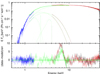 |
Fig. 1. Unfolded average spectrum (0.5–50 keV) of the persistent emission from SRGA J1444. Top panel: merged XMM-Newton RGS (blue points), EPIC-pn (green points) and NuSTAR FPMA and FPMB (black and red points, respectively) are shown as fitted to the semi-phenomenological best-fit model constant*tbabs (bbodyrad + diskbb + nthComp + gauSi + gauAu+ disklineAr + disklineFe)*edge*edge*edge (see Sect. 3.1). Bottom panel: residuals in units of χ with respect to the best-fit model but with the disklineFe component at 6.4 keV removed. |
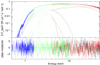 |
Fig. 2. Similar to Fig. 1, but for the reflection model (see text). Top panel: data and spectra for the best-fit continuum model composed of constant*tbabs(bbodyrad + diskbb + nthComp + gauSi+ gauAu+ rdblur*gauAr + rdblur*rfxconv*nthComp)*edge*edge *edge (see Table 1). Bottom panel: residuals in units of χ. |
Alternatively, to retrieve an iron line energy that falls in the Kα iron energy range (i.e., 6.40–6.97 keV) we freeze the inclination parameter of the diskline components to the value obtained by fitting the reflection spectrum, that is 53° (see Sect. 3.2). The remaining best-fit parameters of the iron line model component are the energy of the line,  keV, the Betor parameter,
  , and the inner disk radius, 6.0+0.3 Rg, where the lower value is pegged to the model limit of 6 Rg (see, e.g., Cackett et al. 2010). Employing this iron diskline component brings the test statistic to χ2/d.o.f. = 1329/722 (where d.o.f. refers to the degrees of freedom) with respect to a fit statistic of χ2/d.o.f. = 1735/724 where the iron diskline component was not taken into account in the model.
3.2. Modeling reflection
We fit XMM-Newton and NuSTAR spectral data with a reflection model modified by several components. The dominant components are those described in Sect. 3.1 to which, motivated by the presence of a broadened iron line, we added a reflection component. We account for the reflected component using the convolution model rfxconv (Done & Gierliński 2006) with the relativistic blurring kernel rdblur. The rfxconv model parameters are the relative normalization of the reflection component, the iron abundance (relative to solar ones), the cosine of the disk inclination angle, and the ionization parameter, while the rdblur parameters are, similarly to the diskline component described in Sect. 3.1, the parameter Betor, the inner and outer disk radii, and the disk inclination. We therefore modeled the Ar XVIII line at 3.3 keV with a rdblur*gauss model, which is equivalent to the diskline component, linking the rdblur parameters to those of the reflection component. The inclusion of this component implies a further reduction with respect to the semi-phenomenological model to χ2/d.o.f. = 881/719. A visualization of the reflection features accounted by this component is shown in Fig. 3. Based on the F-test, the probability of chance improvement due to the inclusion of the rfxconv component is 10−63. The resulting best-fit model is thus constant*tbabs(bbodyrad + diskbb + nthComp + gauSi+ gauAu+ rdblur*gauAr + rdblur*rfxconv*nthComp)*edge*edge*edge in XSPEC terminology.
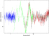 |
Fig. 3. Residuals of the model shown in Fig. 2 with the reflection component removed. Several spectral features are evident, including the iron line at 6.4 keV (see text). |
As a sanity check, we also tested the spectral fit results by ignoring the data in the iron Kα energy band (4.5–8.0 keV) and refitting the data. The resulting iron abundance remains low (on the order of 20%), although the high-energy hump due to reflection remains important. This is in agreement with results from García et al. (2022) of X-ray reflection spectra explored at different iron abundances, which show that the high-energy hump is almost insensitive to the iron abundance, especially for low abundances and low ionization parameter values. For completeness, we also checked the alternative procedure in which we freeze the iron abundance to the Solar one and repeated the fitting procedure excluding spectral data in the iron Kα energy band. This fit gives χ2/d.o.f. = 769/623, but the Ar line around 3.3 keV shows a width of σ ∼ 0.8 keV, too large to be an atomic spectral feature. Also, the Betor parameter is pegged at its minimum value of −10. If data around the iron line energy are included back then χ2 = 9234, with significant negative residuals showing up, indicating that the model over-predicts the line intensity due to the fixed abundance and the high (absolute) value of Betor, which makes the emissivity of the inner disk drastically growing. Upon re-fitting the spectra we obtain χ2/d.o.f. = 1038/720, and the reflected fraction drops to −0.2, while the parameter Betor settles at −2.5. We therefore adopted the best-fit model described above. Our best-fit spectral analysis results are reported in Table 1.
Best-fit parameters of SRGA J1444 data from XMM-Newton (RGS and PN) +NuSTAR observations of the persistent emission fit jointly.
4. X-ray type-I bursts and time-resolved analysis
AMSPs typically exhibit thermonuclear (type-I) X-ray bursts by unstable burning of accreted matter on the NS surface. To search for type-I bursts in our observations, we extracted 10 s-bin light curves from the barycentered XMM-Newton EPIC-pn and NuSTAR events. XMM-Newton light curve was then corrected using the epiclccorr task to correct for energy- and time-dependent loss of events. We found 23 bursts in NuSTAR and 13 in XMM-Newton data. Of these, 9 bursts were observed with both instruments (see Fig. 4). We then performed time-resolved spectroscopy of the brightest burst observed simultaneously with XMM-Newton EPIC-pn and NuSTAR that, at the same time, happens far from the NuSTAR GTI borders. This is burst number 4 in Fig. 4, although we notice here that all bursts throughout the observations considered in this work have similar brightness and recurrence times within ∼10%. For this, we generated variable-length GTIs according to the burst stage, with shorter GTIs around the peak and longer GTIs during the rise and decay phase. More specifically, to ensure comparable statistics in all bins, we extracted 4-s length GTIs in the first and last two bins, 3-s GTIs in the third and fourth to last bins, and 2-s GTIs in all others. We then proceeded to extract source spectra, while we used the persistent source emission spectrum of each instrument obtained in Sect. 3 as a background spectrum. For EPIC-pn spectra, we minimized pile-up effects adopting the same method as described in Sect. 2.2.
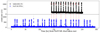 |
Fig. 4. Light curve of SRGA J1444 as observed by NuSTAR (bottom) and XMM-Newton PN (top) at a time binning of 10 s. Contemporaneously observed type-I bursts are marked with a red vertical dashed line and numbered in the top panel for clarity. |
Time-resolved spectra over the burst were modeled with an absorbed blackbody component with variable temperature and radius over the burst evolution (see Fig. 5), similar to Molkov et al. (2024). The persistent emission modeled in Sect. 3.2 was employed as the background spectrum. This model describes the spectra with reduced χ2 ≈ 1.0 for all time-resolved bins. The burst reaches a peak flux of 1.2 × 10⁻⁸ erg cm−2 s−1 in the 0.5–60 keV band, corresponding to a luminosity of 9.3 × 1037 erg s−1 (assuming a distance of 8 kpc). The blackbody temperature evolves rapidly peaking at about 2.7 keV around the peak of the burst flux and then decreasing steadily. The blackbody radius increases from about 5 km to about 7.5 km around 20 s after the outburst onset (similar to that obtained by Molkov et al. 2024). The data do not show evidence of photospheric radius expansion (PRE). Assuming the empirical Eddington luminosity for hydrogen-poor material of 3.8 × 1038 erg s−1 (Kuulkers et al. 2003), we estimated an upper limit on the source distance of about 11.5 kpc (in accordance with the upper limit of 10.6 kpc, Ng et al. 2024).
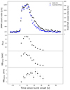 |
Fig. 5. Top panel: light curve of the type-I X-ray burst number 4 (see Fig. 4) observed by EPIC-pn (0.3–10 keV, black dots) and NuSTAR (3–79 keV, blue dots). The unabsorbed flux is traced in the panel below in units of 10−8 erg cm−2 s−1 (0.01–15 keV). The burst onset took place at MJD 60368.49178. The temperature and the apparent radius (for a source distance of 8 kpc) of the blackbody component are plotted in the two bottom panels. |
In the peak of the outburst of SRGA J1444 the burst recurrence time Δt was increasing with the simultaneously decreasing persistent flux from ∼1.6 h to ∼2.9 h (Molkov et al. 2024; Sanchez-Fernandez et al. 2024a,b). Successively, the recurrence time was measured to increase up to ∼8 h at the end of the IXPE observation (Papitto et al. 2025). It is typically observed that

where C is the persistent count rate observed right before the burst, K is a proportionality constant, while β is the power-law index. Typical measured values of the power-law index are β ∼ 1 (Falanga et al. 2011; Bagnoli et al. 2013). Observations of SRGA J1444 also have resulted in β ∼ 0.8–1.0 (Molkov et al. 2024; Papitto et al. 2025; Takeda et al. 2024). With the continuous XMM-Newton observation of SRGA J1444 we are able to infer the best-fit parameters of Eq. (1) without any assumption on the observed quantities (Δt and C) deriving from data gaps that can sometimes affect other instruments. Our results are shown in Fig. 6. Contrary to previous works, we find a power-law index value of β ∼ 0.5. We compare our best-fit results to those obtained by Papitto et al. (2025) by fitting our data with Eq. (1). For this, in Fig. 6 we also plot the power-law index derived in their work (fitting only the proportional constant K).
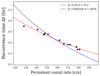 |
Fig. 6. Variation of the recurrence time as a function of the XMM-Newton EPIC-pn persistent count rate. The red dashed line represents a fit of data points to Eq. (1). The blue dashed line represents the fit with β value fixed to 0.8 (see text). |
5. Discussion and conclusions
We have analyzed XMM-Newton and NuSTAR observations of the ASMP SRGA J1444 during its 2024 outburst. Our main findings are summarized and discussed in the following sections.
5.1. Discovery of a relativistic iron line
We fitted the persistent emission employing a semi-phenomenological continuum spectral model consisting of a Comptonized component plus two blackbody components, without modeling the reflection component. This model suggests the presence of a relativistically broadened iron emission line, observed for the first time in this source. When this feature is modeled with a diskline component and all line parameters are let free, the best-fit energy of the line is 6.2 keV. This is only marginally consistent with neutral iron, contrary to the higher ionization regime implied by the identification of a possible Fe XXVI edge in the spectrum. Nonetheless, low-state iron lines at 6.2 keV have been reported in other systems, such as the black holes Cyg X-1 and XTE J1720−318 (Barr et al. 1985; Markwardt 2003), and in the double pulsar system J0737−3039 (Egron et al. 2017). In any case, by freezing the inclination value parameter of the model used to fit the iron line to the same value obtained by the reflection best-fit model (that is 53°) we recover the best-fit energy of the line at 6.4 keV. We identify this line with the iron Kα line of FeI-XV. This is consistent with the relatively low ionization parameter (log ξ ≃ 2.3) obtained from the reflection model employed in Sect. 3.2, although it is in contrast with the possible detection of a Fe XXVI edge discussed more in detail in Sect. 5.2. The best-fit parameters of the blurred line component imply a truncated accretion disk at 6 Rg when the inclination of the system is frozen at 53°, which is the inclination value obtained by fitting the reflection spectrum (see Sect. 3.2), and employed in order to obtain a best-fit value of the iron line energy that is consistent with the Kα iron energy range. Alternatively, a fit where the system inclination is let as a free parameter returns  deg, in broad agreement with polarization measurements of the source which find
  deg (Papitto et al. 2025), and an inner disk radius of
  . A possible, qualitative scenario to ease the tension is that of a disk being more inclined in the inner region, where the polarization measurements come from, with the reflection contribution being more relevant from more distant, less inclined parts of the disk. On the other hand, the discrepancy in the values of the inner disk radius derived from the two fitting procedures is likely a result of the parameters degeneracy. In fact, both inclination and inner disk radius play a major role in shaping the resulting iron line flux and shape (Fabian et al. 1989; George & Fabian 1991), and the observed discrepancy is rather due to the model-driven dependence of the two parameters.
5.2. The reflection spectrum
The persistent source emission can also be fitted with a Comptonized spectrum modified by a reflection component deriving from the accretion disk. A number of discrete features, both instrumental and physical, are observed in the broadband spectrum, supporting the interpretation of a highly ionized reflecting medium. The best-fit parameters reveal a moderately hot (kTe ≈ 20 keV) medium with a thermal component at kTseed ≈ 1 keV emitted by a region on the NS with 11 d8 km radius (where d8 is the source distance in units of 8 kpc), and a hard component interpreted as reflection by the accretion disk at an apparent inner radius of  km, that is
  km (where Ndiskbb is the normalization of the diskbb spectral component, and i = 53°, see Table 1). This is significantly larger than the internal radius value of the accretion disk pegged at the lower limit of 6Rg as obtained from the best fit of the reflection model, considering that the definition of the gravitational radius adopted in the model is Rg = GMNS/c2 ≃ 2 km for a NS mass of 1.4 M⊙. However, such inconsistency between the two methods of retrieving the inner disk radius is often observed throughout the literature (see, e.g., Cackett et al. 2010; Ludlam et al. 2017). This is typically attributed to possible boundary layer corrections and other factors (Kubota et al. 2001), including the scattering of photons off the line of sight by the accretion disk, with the net effect of reducing the contribution of the blackbody component of the disk and thus the inferred apparent radius. We also notice that the relatively low plasma temperature (kTe ≃ 20 keV) observed here is consistent with polarimetric predictions by Bobrikova et al. (2023), as measured by Papitto et al. (2025).
The reflected component implies a subsolar iron abundance (despite a prominent iron emission line, see also later), with a blurring convolution that returns an inclination of 53°. This is in agreement with previous results obtained by modeling of the pulsed emission, which gives an inclination of 58° and an internal disk radius of 24.6 km (Molkov et al. 2024), for which they estimate an error of less than 10%, but significantly deviating from the value obtained by modeling of the phase-resolved polarized emission which returned an inclination of  deg (Papitto et al. 2025). Moreover, assuming that the emitting region distance is coincident with the inner disk radius, we can use the definition of ξ to infer the inner disk radius, that is ξ = LX/(nH Rin2) (Tarter et al. 1969). The bolometric LX luminosity can be obtained by the bolometric flux reported in Table 1 as 2.5 × 1037 erg s−1 at a distance of 8 kpc. A typical Shakura-Sunyaev disk has density nH ∼ 5 × 1020 cm−3 (see, e.g., Ross & Fabian 2007). This results in an inner radius of about 150 km, much larger than the value estimated above. This difference can be mitigated considering that the luminosity irradiating the disk is inferior to bolometric luminosity by a geometry-dependent factor ζ (Zdziarski & De Marco 2020), and assuming a slightly higher disk density, e.g., nH = 6 × 1020 cm−3, which results in an inner radius of 40 ± 4 km. However, we notice that the inner disk radius for a 447.9 Hz pulsar cannot be significantly larger than the corotation radius of 28.6
 km.
km.
The fit also requires a broad gaussian emission line at a centroid energy of about 3.3 keV, which we identify with Ar XVIII. Its large width is likely due to relativistic smearing, as supported by the iron emission line shape (see Sect. 3.1). However, the reflection component should already account for emission lines from ionized elements, such as the Ar XVIII, but also those corresponding to typically more abundant elements such as Si XIV and S XVI. The fact that our best-fit model requires an additional gaussian emission component only for the Ar XVIII is therefore unexpected. We interpret this as probably due to the relatively low best-fit ionization parameter, which makes the Ar line computed from the reflection component alone not intrinsically strong enough to account for the actual observed line, thus requiring an additional component. We also notice the peculiar absorption edge at 9.68 keV. Nominally, this energy value would be consistent with a Zn edge at 9.65 keV. However, the low abundance of Zn makes it highly unlikely. On the other hand, the presence of Ar XVIII argues for highly ionized elements and is therefore in agreement with the presence of Fe XXVI. If the feature actually originates from Fe XXVI, the difference between the nominal (9.278 keV) and the observed (9.68 keV) energy can be interpreted in terms of a blueshifted wind feature. Similar features characteristic of an outflowing wind have been observed in other AMSPs as well (Degenaar et al. 2017; Allen et al. 2018; Nowak et al. 2019), and in other high-inclination systems (see, e.g., Reeves et al. 2004). The resulting outflow speed of ∼13 000 km s−1, that is ∼4% the speed of light, would place such a wind in the regime of ultrafast outflows (Miller et al. 2015, 2016). This is in agreement with the observed low ionization parameter of the reflecting medium, which facilitates radiation pressure acceleration, although it clashes with the very interpretation of a fully ionized iron state. The low iron abundance derived by the reflection model may resolve this tension if iron has a subsolar abundance, but other elements do not. This is especially interesting given the preliminary evidence for the non-solar elemental composition in SRGA J1444 (Dohi et al. 2024). In particular, Dohi et al. (2024) provide evidence of high ZCNO abundances compared to solar values. Carbon-enhanced metal poor (CEMP) stars are a distinct population of stars in their main sequence or giant phase, often found in binary systems (Cooke & Madau 2014; Hirai et al. 2025). This is consistent with the M-type main-sequence companion star suggested for SRGA J1444 (Ng et al. 2024). If confirmed, this would be the first time a CEMP star is observed feeding a compact object.
5.3. Burst energetics
The broadband time-resolved analysis of type-I bursts does not show evidence of photospheric expansion. The recurrence time Δt, which can be accurately estimated thanks to XMM-Newton continuous observation, reveals a dependence on the persistent count rate that is milder than previously observed. We ascribe the observed difference to different factors. First, the narrow interval of Δt covered by our observations can affect the best-fit results. Second, we notice the hysteresis in Fig. 10 of Papitto et al. (2025), where similar count rate values exhibit Δt values that are sensibly different (up to ∼1 h), a condition that can heavily drive the fit results, especially given the above-described factor. Third, there might be a physical reason behind the power-law index difference due to the different energy bands explored and a possible evolution of the spectrum over the outburst, although no clear evidence for this has been observed so far (Gilfanov et al. 1998; Gierliński & Poutanen 2005; Poutanen 2006).
By combining the observed parameters of persistent and burst emission, our data set allows us to obtain the α-value (see Galloway et al. 2022 for the definitions employed below), that is, the ratio of accretion to thermonuclear burning energy:

where Fpers is the bolometric flux of the persistent emission, Eburst is the burst fluence (i.e., the burst flux integrated over the burst time), and Δt is the burst recurrence time. This is important to evaluate the composition of the bursting fuel in terms of the mean hydrogen mass fraction at ignition  . For burst number 4 (see Fig. 4), the total unabsorbed flux (0.01–100 keV) is ∼1.5 × 10⁻⁸ erg cm−2 s−1, which gives a burst fluence of
  erg cm−2, calculated from the time-resolved spectroscopy fluxes (see Sect. 4). We therefore estimate
  for burst number 4. In comparison, Molkov et al. (2024) derive α ≃ 105, although at a different outburst stage, when the composition of the fuel was likely different. On the other hand, the α-value can also be calculated as:
where ξb and ξp are the burst and persistent anisotropy factors accounting for any beaming effects. Qgrav and Qnucl are the accretion and burst energy generation per unit mass, respectively. Following Galloway et al. (2022), Qgrav = c2z(1 + z)≈GMNS/RNS, with z being gravitational redshift that, for a typical NS of mass MNS = 1.4 M⊙ and radius RNS = 11.2 km, is z = 0.259. Thus Qgrav ≈ 190 MeV nucleon−1. On the other hand, the exact value of Qnucl depends on the fuel composition and, for a mixed H/He layer, the approximate expression  MeV nucleon−1 has been recently adopted (Goodwin et al. 2019). Provided that the α-value is known by observational means as done above through Eq. (2), then by substituting the approximate expression for Qnucl in Eq. (3) one can obtain the following (Galloway et al. 2022):
Assuming ξb/ξp on the order of unity, we thus obtain  . This would imply a heavily H-depleted fuel (with respect to solar abundances
  ). The resulting burst energy generation is therefore Qnucl = 3.16 MeV nucleon−1. While the burst is likely burning a mix of H/He, during the persistent emission steady H-burning via hot-CNO cycle is happening. The time scale for this is (10–15 h)(X0/0.7)(ZCNO/0.02)−1(1 + z), where X0 is the fraction of the accreted hydrogen mass (Lampe et al. 2016). This is significantly longer than the burst observed recurrence time, consistent with observations of He bursts taking place in a medium where H has not been completely depleted. However, the H abundance we observed (X = 0.3) is much lower than what would be expected after a ≥2 hours recurrence time. This might hint at a subsolar H fraction of the accreted material.
We can also estimate the burst ignition depth (see Galloway et al. 2022, Eq. 4):
obtaining a value of yign = 0.17 ξb d82 108 g cm−2. We can then evaluate the expected value of the recurrence time as  , where
 ![$ \dot{m}=L_{\mathrm{pers}}(1+z)/[4\pi R_{\mathrm{NS}}^2(GM_{\mathrm{NS}}/R_{\mathrm{NS}})] $](/articles/aa/full_html/2025/07/aa54075-25/aa54075-25-eq57.gif) is the local accretion rate. We obtain
is the local accretion rate. We obtain  g s−1 which, in turn, returns an expected recurrence time of Δt = 2765 s. This is about a factor of three smaller than the observed average value of 2.4 h. A similar discrepancy between the expected and observed value of the recurrence time was also obtained by Falanga et al. (2012) for the AMSP system IGR J17498−2921, attributed to peculiar fuel composition (decreased CNO or X0) combined with an overestimation of the isotropic luminosity. An even lower H fraction than indicated by the burst energetics would increase the burst energy generation rate and the burst ignition depth, so leading to a longer expected burst recurrence rate. If the bursts were taking place in a pure He environment (i.e., X = 0), the expected recurrence time at the observed count rate would amount to ∼1.85 h, much closer to the observed value. Alternatively, such a discrepancy can be mitigated if the persistent emission is beamed toward the observer (that is, ξp < 0.5), or if a larger gravitational redshift is taken into account due to a massive NS as suggested for SRGA J1444 (Takeda et al. 2024).
Acknowledgments
C.M., A.P., G.I., and R.L.P are supported by INAF (Research Grant ‘Uncovering the optical beat of the fastest magnetised neutron stars 620 (FANS)’) and the Italian Ministry of University and Research (MUR) (PRIN 2020, Grant 2020BRP57Z, ‘Gravitational and Electromagnetic-wave Sources in the Universe with current and next-generation detectors (GEMS)’). A.P. acknowledges support from the Fondazione Cariplo/Cassa Depositi e Prestiti, grant no. 2023-2560. J.P. was supported by the Ministry of Science and Higher Education grant 075-15-2024-647. ADM contribution is supported by the Istituto Nazionale di Astrofisica (INAF) and the Italian Space Agency (Agenzia Spaziale Italiana, ASI) through contract ASI-INAF-2022-19-HH.0.
References
- Allen, J. L., Schulz, N. S., Homan, J., et al. 2018, ApJ, 861, 26 [Google Scholar]
- Arnaud, K. A. 1996, ASP Conf. Ser., 101, 17 [Google Scholar]
- Bagnoli, T., in’t Zand, J. J. M., Galloway, D. K., & Watts, A. L. 2013, MNRAS, 431, 1947 [Google Scholar]
- Barr, P., White, N. E., & Page, C. G. 1985, MNRAS, 216, 65P [Google Scholar]
- Barret, D., Olive, J. F., Boirin, L., et al. 2000, ApJ, 533, 329 [Google Scholar]
- Bobrikova, A., Loktev, V., Salmi, T., & Poutanen, J. 2023, A&A, 678, A99 [NASA ADS] [CrossRef] [EDP Sciences] [Google Scholar]
- Cackett, E. M., Miller, J. M., Ballantyne, D. R., et al. 2010, ApJ, 720, 205 [Google Scholar]
- Cash, W. 1979, ApJ, 228, 939 [Google Scholar]
- Cooke, R. J., & Madau, P. 2014, ApJ, 791, 116 [Google Scholar]
- Degenaar, N., Pinto, C., Miller, J. M., et al. 2017, MNRAS, 464, 398 [NASA ADS] [CrossRef] [Google Scholar]
- Di Salvo, T., & Sanna, A. 2022, Astrophys. Space Sci. Libr., 465, 87 [Google Scholar]
- Di Salvo, T., D’Aí, A., Iaria, R., et al. 2009, MNRAS, 398, 2022 [NASA ADS] [CrossRef] [Google Scholar]
- Di Salvo, T., Iaria, R., Matranga, M., et al. 2015, MNRAS, 449, 2794 [NASA ADS] [CrossRef] [Google Scholar]
- Di Salvo, T., Sanna, A., Burderi, L., et al. 2019, MNRAS, 483, 767 [NASA ADS] [CrossRef] [Google Scholar]
- Diez, C. M., Grinberg, V., Fürst, F., et al. 2023, A&A, 674, A147 [NASA ADS] [CrossRef] [EDP Sciences] [Google Scholar]
- Dohi, A., Nishimura, N., Hirai, R., et al. 2024, PASJ, in press [arXiv:2411.10993] [Google Scholar]
- Done, C., & Gierliński, M. 2006, MNRAS, 367, 659 [NASA ADS] [CrossRef] [Google Scholar]
- Egron, E., Pellizzoni, A., Pollock, A., et al. 2017, ApJ, 838, 120 [Google Scholar]
- Fabian, A. C., Rees, M. J., Stella, L., & White, N. E. 1989, MNRAS, 238, 729 [Google Scholar]
- Falanga, M., Kuiper, L., Poutanen, J., et al. 2011, A&A, 529, A68 [NASA ADS] [CrossRef] [EDP Sciences] [Google Scholar]
- Falanga, M., Kuiper, L., Poutanen, J., et al. 2012, A&A, 545, A26 [NASA ADS] [CrossRef] [EDP Sciences] [Google Scholar]
- Galloway, D. K., Muno, M. P., Hartman, J. M., Psaltis, D., & Chakrabarty, D. 2008, ApJS, 179, 360 [NASA ADS] [CrossRef] [Google Scholar]
- Galloway, D. K., Johnston, Z., Goodwin, A., & He, C.-C. 2022, ApJS, 263, 30 [NASA ADS] [CrossRef] [Google Scholar]
- García, J. A., Dauser, T., Ludlam, R., et al. 2022, ApJ, 926, 13 [CrossRef] [Google Scholar]
- George, I. M., & Fabian, A. C. 1991, MNRAS, 249, 352 [Google Scholar]
- Gierliński, M., & Poutanen, J. 2005, MNRAS, 359, 1261 [Google Scholar]
- Gierliński, M., Done, C., & Barret, D. 2002, MNRAS, 331, 141 [CrossRef] [Google Scholar]
- Gilfanov, M., Revnivtsev, M., Sunyaev, R., & Churazov, E. 1998, A&A, 338, L83 [NASA ADS] [Google Scholar]
- Goodwin, A. J., Heger, A., & Galloway, D. K. 2019, ApJ, 870, 64 [NASA ADS] [CrossRef] [Google Scholar]
- Harrison, F. A., Craig, W. W., Christensen, F. E., et al. 2013, ApJ, 770, 103 [Google Scholar]
- Hirai, Y., Saitoh, T. R., Fujii, M. S., Kaneko, K., & Beers, T. C. 2025, ApJ, 980, L25 [Google Scholar]
- Illiano, G., Coti Zelati, F., Marino, A., et al. 2024a, ATel., 16510, 1 [Google Scholar]
- Illiano, G., Papitto, A., Marino, A., et al. 2024b, A&A, 691, A189 [NASA ADS] [CrossRef] [EDP Sciences] [Google Scholar]
- Kaastra, J. S., & Bleeker, J. A. M. 2016, A&A, 587, A151 [NASA ADS] [CrossRef] [EDP Sciences] [Google Scholar]
- Kubota, A., Makishima, K., & Ebisawa, K. 2001, ApJ, 560, L147 [NASA ADS] [CrossRef] [Google Scholar]
- Kuulkers, E., den Hartog, P. R., in’t Zand, J. J. M., et al. 2003, A&A, 399, 663 [NASA ADS] [CrossRef] [EDP Sciences] [Google Scholar]
- Lampe, N., Heger, A., & Galloway, D. K. 2016, ApJ, 819, 46 [NASA ADS] [CrossRef] [Google Scholar]
- Ludlam, R. M., Miller, J. M., Degenaar, N., et al. 2017, ApJ, 847, 135 [NASA ADS] [CrossRef] [Google Scholar]
- Makishima, K. 1986, Lecture Notes Phys., 266, 249 [Google Scholar]
- Markwardt, C. B. 2003, ATel., 115, 1 [Google Scholar]
- Mereminskiy, I. A., Semena, A. N., Molkov, S. V., et al. 2024, ATel., 16464, 1 [Google Scholar]
- Miller, J. M., Fabian, A. C., Kaastra, J., et al. 2015, ApJ, 814, 87 [NASA ADS] [CrossRef] [Google Scholar]
- Miller, J. M., Raymond, J., Cackett, E., Grinberg, V., & Nowak, M. 2016, ApJ, 822, L18 [NASA ADS] [CrossRef] [Google Scholar]
- Molkov, S. V., Lutovinov, A. A., Tsygankov, S. S., et al. 2024, A&A, 690, A353 [NASA ADS] [CrossRef] [EDP Sciences] [Google Scholar]
- Ng, M., Ray, P. S., Sanna, A., et al. 2024, ApJ, 968, L7 [NASA ADS] [CrossRef] [Google Scholar]
- Nowak, M. A., Paizis, A., Jaisawal, G. K., et al. 2019, ApJ, 874, 69 [NASA ADS] [CrossRef] [Google Scholar]
- Papitto, A., Di Salvo, T., D’Aì, A., et al. 2009, A&A, 493, L39 [NASA ADS] [CrossRef] [EDP Sciences] [Google Scholar]
- Papitto, A., Riggio, A., di Salvo, T., et al. 2010, MNRAS, 407, 2575 [Google Scholar]
- Papitto, A., Di Marco, A., Poutanen, J., et al. 2025, A&A, 694, A37 [NASA ADS] [CrossRef] [EDP Sciences] [Google Scholar]
- Patruno, A., & Watts, A. L. 2021, ASSL, 461, 143 [NASA ADS] [Google Scholar]
- Pavlinsky, M., Tkachenko, A., Levin, V., et al. 2021, A&A, 650, A42 [EDP Sciences] [Google Scholar]
- Pintore, F., Sanna, A., Di Salvo, T., et al. 2016, MNRAS, 457, 2988 [NASA ADS] [CrossRef] [Google Scholar]
- Poutanen, J. 2006, Adv. Space Res., 38, 2697 [Google Scholar]
- Reeves, J. N., Porquet, D., & Turner, T. J. 2004, ApJ, 615, 150 [Google Scholar]
- Ross, R. R., & Fabian, A. C. 2007, MNRAS, 381, 1697 [NASA ADS] [CrossRef] [Google Scholar]
- Saavedra, E. A., Fogantini, F. A., Escobar, G. J., et al. 2023, A&A, 680, A88 [NASA ADS] [CrossRef] [EDP Sciences] [Google Scholar]
- Sanchez-Fernandez, C., Kuulkers, E., Ferrigno, C., & Chenevez, J. 2024a, ATel., 16485, 1 [Google Scholar]
- Sanchez-Fernandez, C., Kuulkers, E., Ferrigno, C., Chenevez, J., & Del Santo, M. 2024b, ATel., 16507, 1 [Google Scholar]
- Snios, B., Siemiginowska, A., Sobolewska, M., et al. 2020, ApJ, 899, 127 [NASA ADS] [CrossRef] [Google Scholar]
- Strohmayer, T., & Bildsten, L. 2006, in Compact stellar X-ray sources, Cambridge Astrophysics Series, eds. W. Lewin, & M. van der Klis, 39 (Cambridge: Cambridge University Press), 113 [NASA ADS] [Google Scholar]
- Sunyaev, R., Arefiev, V., Babyshkin, V., et al. 2021, A&A, 656, A132 [NASA ADS] [CrossRef] [EDP Sciences] [Google Scholar]
- Takeda, T., Tamagawa, T., Enoto, T., et al. 2024, PASJ, 77, L24 [Google Scholar]
- Tarter, C. B., Tucker, W. H., & Salpeter, E. E. 1969, ApJ, 156, 943 [Google Scholar]
- Wilms, J., Allen, A., & McCray, R. 2000, ApJ, 542, 914 [Google Scholar]
- Zdziarski, A. A., & De Marco, B. 2020, ApJ, 896, L36 [NASA ADS] [CrossRef] [Google Scholar]
- Zdziarski, A. A., Johnson, W. N., & Magdziarz, P. 1996, MNRAS, 283, 193 [NASA ADS] [CrossRef] [Google Scholar]
- Życki, P. T., Done, C., & Smith, D. A. 1999, MNRAS, 309, 561 [Google Scholar]
All Tables
Best-fit parameters of SRGA J1444 data from XMM-Newton (RGS and PN) +NuSTAR observations of the persistent emission fit jointly.
All Figures
|
Fig. 1. Unfolded average spectrum (0.5–50 keV) of the persistent emission from SRGA J1444. Top panel: merged XMM-Newton RGS (blue points), EPIC-pn (green points) and NuSTAR FPMA and FPMB (black and red points, respectively) are shown as fitted to the semi-phenomenological best-fit model constant*tbabs (bbodyrad + diskbb + nthComp + gauSi + gauAu+ disklineAr + disklineFe)*edge*edge*edge (see Sect. 3.1). Bottom panel: residuals in units of χ with respect to the best-fit model but with the disklineFe component at 6.4 keV removed. |
| In the text | |
|
Fig. 2. Similar to Fig. 1, but for the reflection model (see text). Top panel: data and spectra for the best-fit continuum model composed of constant*tbabs(bbodyrad + diskbb + nthComp + gauSi+ gauAu+ rdblur*gauAr + rdblur*rfxconv*nthComp)*edge*edge *edge (see Table 1). Bottom panel: residuals in units of χ. |
| In the text | |
|
Fig. 3. Residuals of the model shown in Fig. 2 with the reflection component removed. Several spectral features are evident, including the iron line at 6.4 keV (see text). |
| In the text | |
|
Fig. 4. Light curve of SRGA J1444 as observed by NuSTAR (bottom) and XMM-Newton PN (top) at a time binning of 10 s. Contemporaneously observed type-I bursts are marked with a red vertical dashed line and numbered in the top panel for clarity. |
| In the text | |
|
Fig. 5. Top panel: light curve of the type-I X-ray burst number 4 (see Fig. 4) observed by EPIC-pn (0.3–10 keV, black dots) and NuSTAR (3–79 keV, blue dots). The unabsorbed flux is traced in the panel below in units of 10−8 erg cm−2 s−1 (0.01–15 keV). The burst onset took place at MJD 60368.49178. The temperature and the apparent radius (for a source distance of 8 kpc) of the blackbody component are plotted in the two bottom panels. |
| In the text | |
|
Fig. 6. Variation of the recurrence time as a function of the XMM-Newton EPIC-pn persistent count rate. The red dashed line represents a fit of data points to Eq. (1). The blue dashed line represents the fit with β value fixed to 0.8 (see text). |
| In the text | |
Current usage metrics show cumulative count of Article Views (full-text article views including HTML views, PDF and ePub downloads, according to the available data) and Abstracts Views on Vision4Press platform.
Data correspond to usage on the plateform after 2015. The current usage metrics is available 48-96 hours after online publication and is updated daily on week days.
Initial download of the metrics may take a while.