| Issue |
A&A
Volume 698, June 2025
|
|
|---|---|---|
| Article Number | A199 | |
| Number of page(s) | 11 | |
| Section | Planets, planetary systems, and small bodies | |
| DOI | https://doi.org/10.1051/0004-6361/202555145 | |
| Published online | 17 June 2025 | |
Modeling helium in exoplanet atmospheres. A revised network with photoelectron-driven processes
Université Paris-Saclay, Université Paris Cité, CEA, CNRS, AIM,
91191,
Gif-sur-Yvette,
France
★ Corresponding author: This email address is being protected from spambots. You need JavaScript enabled to view it.
Received:
13
April
2025
Accepted:
15
May
2025
Abstract
Context. The He I line at 1.08 μm is a valuable tracer of atmospheric escape in exoplanet atmospheres.
Aims. We expand past networks used to predict the absorbing He(23S) by including, firstly, processes that involve H2 and some molecular ions, and secondly, the interaction of photoelectrons with the atmosphere.
Methods. We survey the literature on the chemical-collisional-radiative processes that govern the production-loss of He(23S). We simulate the atmospheric outflow from the Neptune-sized GJ 436 b by coupling a hydrodynamic model that solves the bulk properties of the gas and a Monte Carlo model that tracks the energy degradation of the photoelectrons.
Results. We identify Penning ionization of H as a key He(23S) loss process at GJ 436 b and update its rate coefficient to a value consistent with the most recent available cross sections. The update significantly affects the predicted strength of the He I line. For GJ 436 b, photoelectron-driven processes (mainly ionization and excitation) modify the He(23S) population in layers too deep to affect the in-transit spectrum. The situation might be different for other atmospheres though. The spectral energy distribution of the host star GJ 436 has a strong effect on the predicted in-transit signal. The published nondetections of the He I line for GJ 436 b are reasonably consistent with our model predictions for a solar-metallicity atmosphere when the model adopts a recently proposed spectral energy distribution for the star.
Conclusions. The interpretation of the He I line at 1.08 μm is model dependent. Our revised network provides a general framework for extracting more robust conclusions from measurements of this line, especially in atmospheres where H2 remains abundant to high altitudes. We will explore additional, previously ignored processes in future work.
Key words: planets and satellites: atmospheres
© The Authors 2025
 Open Access article, published by EDP Sciences, under the terms of the Creative Commons Attribution License (https://creativecommons.org/licenses/by/4.0), which permits unrestricted use, distribution, and reproduction in any medium, provided the original work is properly cited.
This article is published in open access under the Subscribe to Open model. This email address is being protected from spambots. You need JavaScript enabled to view it. to support open access publication.
1 Introduction
Atmospheric escape plays a key role in the evolution of exoplanets (Owen 2019; Bean et al. 2021). Diagnostic lines that trace the escaping gas and that can be probed with current technology, such as those in the H I Balmer series (Yan & Henning 2018) or the He I line at 1.08 μm, are enormously advancing our understanding of atmospheric escape. The history of the latter is particularly interesting. Modeling by Seager & Sasselov (2000) and Turner et al. (2016) suggests that it was detectable at some close-in exoplanets. However, it took almost two decades for the first detection in the in-transit spectrum of an exoplanet to be reported (Spake et al. 2018). Since then, the He I line at 1.08 μm has been identified at ~20 exoplanets and remains a priority in spectroscopic surveys (Vissapragada et al. 2022; Fossati et al. 2023; Guilluy et al. 2024; Masson et al. 2024; Sanz-Forcada et al. 2025). As observations of this line continue, it becomes more important to assess its diagnostic value and how its strength is affected by the planet-star properties.
Oklopčić & Hirata (2018) lay out a network of processes that populate the metastable state absorbing in the He(23S)+hν (1.08 μm)→He(23P) line. In short, photoionization by energetic stellar photons creates He+ ions that recombine with the thermal electrons. A fraction of the recombinations end up as He(23S) that, not being connected with the ground state through dipole emission, builds up to potentially detectable amounts. Subsequent models adopted this network with little variation (e.g., Oklopčić 2019; Czesla et al. 2022; Dos Santos et al. 2022; Yan et al. 2022; Lampón et al. 2023; Rumenskikh et al. 2023; Biassoni et al. 2024; Allan et al. 2024; Schreyer et al. 2024; Ballabio & Owen 2025). Taking a step back, we aim to assess the completeness of the network. In particular, in this first work, we expand the network to accommodate interactions with H2 and some molecular ions, and explore to what extent photoelectrondriven processes affect the He(23S) population, directly or indirectly. In later work, we will explore other aspects of the modeling, such as the importance of in-detail radiative transfer in the lines and the continuum, or the role of chemical reactions with a variety of elements.
We define by photoelectrons or primaries the electrons formed from photoionization, and by secondaries the electrons formed as the primaries slow down in ionizing collisions with atoms and molecules. Various works have explored the role of photoelectrons in the energy budget and chemistry of exoplanets (Cecchi-Pestellini et al. 2009; Shematovich et al. 2014; García Muñoz 2023b; Gillet et al. 2023; Locci et al. 2024). However, their effect on diagnostic lines remains largely unexplored (García Muñoz 2023a; Gillet et al. 2025). To our knowledge, and save for some qualitative statements in García Muñoz (2023a), there has been no quantitative study of the effect of photoelectrons on the He I line at 1.08 μm.
We focus on GJ 436 b, a Neptune-sized exoplanet orbiting an M2.5V-type star. The planet has been a recurrent target of observations to characterize its atmosphere and of modeling for their interpretation (e.g., Madhusudhan & Seager 2011; Moses et al. 2013; Knutson et al. 2014; Morley et al. 2017; Grasser et al. 2024; Mukherjee et al. 2025). Given its low density and equilibrium temperature, Teq~ 700 K, the atmospheric layers probed by visible-infrared radiation are likely dominated by H2. Photodissociaton will lead to an H-atom-dominated gas at high altitudes. It is unclear whether the transition from H2- to H-dominated has implications for other aspects of atmospheric chemistry, which remains a path to be explored. The evidence at GJ 436 b for any molecules, such as H2O, CO, CO2, CH4, or SO2, that have been found at other warm exoplanets, remains weak (Grasser et al. 2024; Mukherjee et al. 2025). The nondetection of molecular features can be attributed to the atmosphere having a high metallicity, and therefore a small scale height, or to the occurrence of high-altitude clouds or a combination of both conditions. Identifying the main reason remains an open problem that, once solved, should help us better understand the generality of exoplanet atmospheres. Like other Neptune-sized planets such as HAT-P-11 b and GJ 3470 b, GJ 436 b is enshrouded by a cloud of H atoms escaping the planet and that can be probed by H I Lyman-α absorption spectroscopy (Kulow et al. 2014; Ehrenreich et al. 2015; Bourrier et al. 2018; Ben-Jaffel et al. 2022). Unlike for the other planets, the attempts to detect the He I line at 1.08 μm at GJ 436 b have so far failed (Nortmann et al. 2018; Guilluy et al. 2024; Masson et al. 2024). The nondetection of the He I line is intriguing because the available models predict a strong absorption signal (Oklopčić & Hirata 2018; Dos Santos et al. 2022; Rumenskikh et al. 2023).
2 General formulation
To simulate the escaping atmosphere, we solved the equations of mass, momentum, and energy conservation for the multi-species gas in a spherical-shell geometry. The helium signal peaks relatively close to the planet; therefore, this simplified geometry should be adequate to model the absorbing region. Our numerical model builds upon methods presented previously (García Muñoz 2007; García Muñoz et al. 2021) and those currently under redevelopment to incorporate additional disequilibrium processes (García Muñoz, in prep.). In what follows, we give a brief account of the helium modeling.
The model solves the mass conservation equation
![Mathematical equation: $\[\frac{\partial n_s}{\partial t}+\nabla \cdot \Phi_s=\frac{\delta n_s}{\delta t},\]$](/articles/aa/full_html/2025/06/aa55145-25/aa55145-25-eq1.png) (1)
(1)
where ns [cm−3] is the number density of the species (or particle type) specified by s, Φs [cm−2 s−1] is the flux, and δns/δt [cm−3s−1] is the production or loss rate (if >0 or <0, respectively) due to chemical, collisional, and radiative (Ch-C-R, hereafter) processes. We omitted photoexcitation between bound states driven by absorption of radiation. The implications of this simplification will be investigated in future work on the detailed treatment of radiative transfer. In its current implementation, the network includes about 200 Ch-C-R processes. The momentum conservation equation was treated in a standard way. Energy conservation was formulated by consistently tracking the radiative exchanges (for bound-bound, bound-free, free-bound, and free-free interactions) of the gas with its surroundings (García Muñoz & Schneider 2019).
We focused on purely hydrogen-helium atmospheres made of e− (thermal electrons), ![Mathematical equation: $\[\mathrm{H}(i), \mathrm{H}_2, \mathrm{H}^{+}, \mathrm{H}_2^{+}, \mathrm{H}_3^{+}, \mathrm{He}(i), \mathrm{He}^{+}\]$](/articles/aa/full_html/2025/06/aa55145-25/aa55145-25-eq2.png) , and HeH+. The index, i, specifies the electronic excitation state. The hydrogen chemistry implemented in the model was relatively standard (García Muñoz & Schneider 2019; García Muñoz et al. 2021) and will not be discussed further. The He(i) states are listed in Table A.1. The He(23S) and He(21S) states are metastable. Truncating the He(i) atom model at i≤5 was a reasonable trade-off between expediency and an accurate representation of the cascade that forms upon radiative recombination. We omitted the doubly charged ion He2+ because its density is low under most conditions. A separate form of Eq. (1) was solved for each species.
, and HeH+. The index, i, specifies the electronic excitation state. The hydrogen chemistry implemented in the model was relatively standard (García Muñoz & Schneider 2019; García Muñoz et al. 2021) and will not be discussed further. The He(i) states are listed in Table A.1. The He(23S) and He(21S) states are metastable. Truncating the He(i) atom model at i≤5 was a reasonable trade-off between expediency and an accurate representation of the cascade that forms upon radiative recombination. We omitted the doubly charged ion He2+ because its density is low under most conditions. A separate form of Eq. (1) was solved for each species.
We made a significant effort to revise the Ch-C-R processes relevant to the species listed above, in particular those that contain helium. For example, our network incorporates a variety of processes in which they interact with H2 and the ![Mathematical equation: $\[\mathrm{H}_{2}^{+}, \mathrm{H}_{3}^{+}\]$](/articles/aa/full_html/2025/06/aa55145-25/aa55145-25-eq3.png) , and HeH+ molecular ions that appear as by-products of the H2 chemistry. This was essential for simulating the warm atmospheres of Neptune- and sub-Neptune-sized planets that are likely to retain H2 up to high altitudes. Next, we elaborated on our choices for the Ch-C-R processes participated in by helium-bearing species.
, and HeH+ molecular ions that appear as by-products of the H2 chemistry. This was essential for simulating the warm atmospheres of Neptune- and sub-Neptune-sized planets that are likely to retain H2 up to high altitudes. Next, we elaborated on our choices for the Ch-C-R processes participated in by helium-bearing species.
Photoionization was considered for the He ground and metastable states, with cross sections from the NORAD database (Nahar 2010, 2020). These are presented in Fig. A.1. The structure at 100–400 Å is true and arises from resonances. For the inverse process of radiative recombination, He++e−→He(i)+hν, we calculated effective rate coefficients, αi,eff [cm3s−1], ourselves. Each αi,eff included the contribution, αi, from direct radiative recombination into state i plus the contribution from the cascade that forms from the higher-energy states not explicitly resolved in our atom model and that eventually radiate into state i. Formally, αi,eff=αi+∑j>5αjpji, where pji=Aji/∑i,i≠1 Aji is the probability that emission from state j leads into state i, with the assumption that line opacity prevents radiative decay into the ground state. For the cascade, we borrowed αi and Aji from NORAD. For states with principal quantum number >10, NORAD reports the joint contribution of recombination into singlets and triplets. We assumed a 1:3 partitioning between them and assigned their rates to the states with principal quantum number =10. Table A.2 shows the αi,eff at various temperatures. Recombination into the higher-energy (lower-energy) states becomes prevalent at low (high) temperatures. For implementation, we fitted αi,eff to analytical expressions between 100 and 30 000 K. These fits and others described later are made available in an SI file.
We took the transition probabilities, Aji, for bound-bound transitions from Wiese & Fuhr (2009). Exceptionally, Aji for two-photon He(21S)→He(11S)+hν1+hν2 was from Drake (1986). See Table A.3 for details.
We formed the rate coefficients for (de)excitation of the He(i) states in collisions with thermal electrons from the effective collision strengths, Υji(T), of Berrington & Kingston (1987) at temperatures, T, between 1000 and 5000 K and Bray et al. (2000) between 5600 and 20 000 K. The latter calculations were expected to be more accurate. However, an accurate description of the low temperatures is critical because the He(23S) absorption often occurs in relatively cool layers of the atmosphere. Coincidentally or not, the Υji(T) for deexcitation of the He metastables from both works is consistent. Confirmation of the low-temperature Υji(T) by new calculations is welcomed, to minimize the model uncertainties. Table A.4 shows the rate coefficients at various temperatures. The collisions of charged particles such as H+ or He+ with the He(i) states might conceivably contribute to their (de)excitation. Unfortunately, there seems to be no quantitative information on these collisions at the relevant energies or temperatures. Calculations of this type are also welcomed.
The loss of the He metastables in collisions with neutrals typically proceeds via ionization. Table A.5 lists the dominant processes (Miller et al. 1972; West et al. 1975; Preston & Cohen 1976), as implemented here. For collisions with H and H2, we calculated the rate coefficients from the total ionization cross sections reported in the quoted references to ensure they are reliable from 200 to 10 000 K. For the partitioning of Penning and associative ionization (the latter leads to HeH+), we used an average 0.9:0.1. We note that the literature contains different prescriptions for Penning ionization. For example, Roberge & Dalgarno (1982) quoted a T-independent rate coefficient of 5 × 10⁻¹⁰ cm3 s−1 for Penning ionization of H atoms, while Fassia et al. (1998) proposed 7.5×10⁻¹⁰(T/300)1/2 cm3 s−1 for the same process. For a temperature T=5000 K, representative of exoplanet conditions, the two prescriptions differ by a factor of six. Table A.6 lists additional processes that control the HeH+population.
We consider the charge-exchange processes in Table A.7. These include the loss of He metastables in collisions with H+, with rate coefficients from Loreau et al. (2018) extrapolated to T<3000 K (J. Loreau, priv. comm.). For He++H2, we adopted a rate coefficient based on the Schauer et al. (1989) experiment and assumed that the process leads to H2 dissociation.
The spectral energy distribution (SED) of the host star partly dictates the rate at which photoelectrons are released. Prescriptions of GJ 436’s SED have been presented via the HAbitable Zones and M dwarf Activity across Time (HAZMAT; Peacock et al. 2019), Measurements of the Ultraviolet Spectral Characteristics of Low-mass Exoplanetary Systems (MUSCLES; France et al. 2016) and X-Exoplanets (Sanz-Forcada et al. 2025) programs. There are notable differences among them, and we refer to those references to understand their origin. The HAZMAT SED includes no X-ray information and thus we omit it from our discussion. We repeated all our calculations with both the MUSCLES and the X-Exoplanets SEDs. We extended the X-Exoplanets SED above its original long-wavelength limit of 2800 Å by assuming blackbody emission from the star. The extension introduces an unphysical discontinuity in the SED. As our calculations for GJ 436 b show that photoionization does not dominate the He(21S) loss (the metastable that photoionizes at these wavelengths), we did not attempt an alternative reconstruction. Figure 1 shows both the MUSCLES and X-Exoplanets SEDs at the spectral resolution at which our model calculations were performed.
The boundary conditions in the hydrodynamic model that solves the atmospheric outflow were standard (García Muñoz 2007). The lower boundary was set at a radial distance, Rp, that we took as the planet’s optical radius. We fixed the pressure there to p=1 dyn cm−2, the temperature to Teq, and the volume mixing ratios to values appropriate to solar composition (0.163 for He, a somewhat arbitrary 10−3 for H, and 0 for the other species except H2, which makes up the bulk of the gas). We explored the impact of setting the lower boundary at pressures as high as 100 dyn cm−2. We find this to be relatively minor because, for a temperate planet such as GJ 436 b, the geometric size of the region between 100 and 1 dyn cm−2 is notably less than that of the layer masked by the He I line core.
The hydrodynamic model was coupled to a Monte Carlo model, with which the photoelectron-driven rates for excitation, dissociation, and ionization were calculated (García Muñoz 2023a; García Muñoz & Bataille 2024). Both models communicate with each other until a steady state is attained. In our experience, only a few Monte Carlo calculations are needed to accurately describe the photoelectron effects.
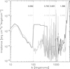 |
Fig. 1 MUSCLES SED (black) and X-Exoplanets SED (gray) at 1 AU and the spectral resolution adopted here. The quoted numbers refer, from left to right, to the integration over the intervals 0→100 Å; 0→503 Å; 0→911 Å; 0→2600 Å, in units of erg cm−2 s−1. |
3 Photoelectron-driven processes
Based on energy considerations, it is apparent that photoelectrons can drive numerous processes that are inaccessible to thermal electrons. Exploring this idea, García Muñoz (2023a) studied some aspects of the photoelectron-driven production and loss of the H(2s) and H(2p) states that are probed via the H I Balmer lines in the in-transit spectra of ultrahot Jupiters (Yan & Henning 2018; Cauley et al. 2021; Czesla et al. 2022). That work finds that, for the exoplanet HAT-P-32 b: i) photoelectron-driven excitation of the H ground state does not dominate the H(2s, 2p) formation where the H I Balmer lines form; ii) the collisions of photoelectrons with H(2s, 2p), whether leading to deexcitation or ionization, affect the lifetimes of these excited states only negligibly; and iii) secondary electrons potentially modify the ionization balance in the atmosphere at altitudes where the H I Balmer lines and the He I line at 1.08 μm are formed. García Muñoz (2023a) does not solve the simultaneous hydrodynamic and photoelectron energy degradation problems, and therefore does not quantify the implications of point iii).
For the present study we revisited and expanded on the above ideas, focusing on the He I line at 1.08 μm at GJ 436 b. In particular, we aimed to quantify the contribution of photoelectrons to: (Q1) the ionization balance of an H2-H-He atmosphere, and how this propagates into the He(23S) population, (Q2) the production of He(23S), either directly from the He ground state or indirectly through excitation of higher-energy states that cascade through bound-bound radiation, (Q3) the He(23S) loss through ionization or deexcitation.
To address these questions, we newly included in the Ch-C-R network the relevant processes for photoelectron-driven (de)excitation, dissociation, and ionization of H2, H, and He. The treatment of H and H2 has been described before (García Muñoz 2023a; García Muñoz & Bataille 2024). The photoelectron-driven processes for He are listed in Table A.8. The cross sections for He excitation and ionization are from Ralchenko et al. (2008) and we inferred the deexcitation ones from detailed balancing. Figure A.2 shows these. Recent experiments by Génévriez et al. (2017) confirm that the adopted He(23S) ionization cross sections are reliable.
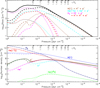 |
Fig. 2 Top: production rates of primary (dashed lines) and secondary (dotted lines) electrons from the MUS-a and -b models. Colors separate the contributions by donor. The dashed black line refers to the primaries summed over all donors. The solid black line refers to the total of primaries and secondaries summed over all donors. Bottom: number densities. Dashed and solid lines refer to MUS-a and -b, respectively. Each panel provides, based on the MUS-b model, the conversion between pressure and radial distance normalized to the planet’s optical radius (r/Rp; =1 at the model’s lower boundary). |
4 Results
To address Q1-Q3, we first ran four models of GJ 436 b. Two models used the MUSCLES SED, the other two used the X-Exoplanets SED. These are identified as MUS-a and MUS-b, and X-Exo-a and X-Exo-b, respectively. Models with the label ‘-a’ (‘-b’) omit (include) the effect of photoelectrons. The MUSCLES SED describes a more strongly emitting star, thereby further enhancing the action of photoelectrons. That is the reason why we prioritize the MUS-a and -b models in the discussion below.
To address Q1, Fig. 2 (top) shows, for the MUS-a and -b models, the rates at which the primary and secondary electrons are released. The dashed colored lines refer to the primaries, separated by process; the dotted colored lines refer to the secondaries, also separated by process; the dashed black line refers to the primaries summed over all processes; and lastly the solid black line refers to the primaries plus secondaries summed over all processes. The relative contribution of the secondaries becomes significant or dominant at p≳10−2 dyn cm−2 (r/Rp≤1.07), where the main donors of primaries are H2 and He and the mean energies of the primaries are 100–300 eV.
For comparison, Fig. 2 (bottom) shows the e−, H2, H, H+, He, He+, and He(23S) densities. Enhanced ionization by the secondaries leads to lower densities of neutrals and higher densities of charged particles. However, the differences in electron densities between the MUS-a and MUS-b models never exceed 50% and they occur preferentially at r/Rp<1.1. At r/Rp~1.1, neutralization proceeds mainly through (fast) dissociative recombination, ![Mathematical equation: $\[\mathrm{H}_{3}^{+}+\mathrm{e}^{-} \rightarrow 3 \mathrm{H}, \rightarrow \mathrm{H}_{2}+\mathrm{H}\]$](/articles/aa/full_html/2025/06/aa55145-25/aa55145-25-eq4.png) , ensuring that the newly formed ions are rapidly replaced by neutrals and thus undoing the initial ionization step. It is likely that the mild atmospheric response to photoelectron-driven ionization seen in Fig. 2 is specific to atmospheres in which molecules remain abundant. Foreseeably, if the atmospheric gas is in atomic form, neutralization will be less efficient because it must proceed through (slow) radiative recombination.
, ensuring that the newly formed ions are rapidly replaced by neutrals and thus undoing the initial ionization step. It is likely that the mild atmospheric response to photoelectron-driven ionization seen in Fig. 2 is specific to atmospheres in which molecules remain abundant. Foreseeably, if the atmospheric gas is in atomic form, neutralization will be less efficient because it must proceed through (slow) radiative recombination.
For reference, Fig. 3 shows the temperature and velocity profiles for both the MUS-b and X-Exo-b models. They are generally lower for the latter, as expected from a weaker stellar irradiation. T~5000 K at the peaks of the He(23S) density.
To address Q2, Fig. 4 (top) shows, for the MUS-b model, the rates of the main He(23S) production processes. Near the He(23S) density peak at p~1.5×10⁻³ dyn cm−2 (r/Rp~1.21), radiative recombination dominates, either directly or indirectly (initially populating He(23P), which decays promptly into He(23S)). Toward the model’s lower boundary, photoelectrondriven excitation from the He ground state dominates. The latter occurs either by direct excitation into He(23S) or by excitation into and subsequent radiative decay from He(23P). The borderline between photoelectron-driven excitation and radiative recombination as the dominant He(23S) production processes is at p~10−2 dyn cm−2. The distinction is important because it defines the source of the He(23S) probed during transit.
Similarly, and to address Q3, Fig. 4 (bottom) shows the rates of the main He(23S) loss processes. Penning ionization of H2 toward the model’s lower boundary and of H near the He(23S) density peak set the He metastable’s lifetime at p≳5×10⁻⁴ dyn cm−2. At lower pressures, aided by temperatures of ~5000 K, excitation into He(21S) and He(23P) in collisions with thermal electrons becomes competitive at removing He(23S). Most He(23P) formed this way will decay back into He(23S). Excitation into He(21S) ensures some singlet-triplet mixing, thus opening new possibilities for the ultimate removal of He(23S). The layers at p~5×10⁻⁴ dyn cm−2 (based on the MUS-a and MUS-b models, see below) are very important because they set the planet’s size at the core of the He I line. It follows that competition between He(23S)+H→ionization and He(23S)+e−→excitation at removing He(23S) introduces a complex dependence on temperature and the H and e− densities in the formation of the line. We note that neither photoionization nor the photoelectron-driven processes (for excitation, deexcitation, or ionization) seem to really affect the He(23S) loss at these low pressures. In the atmospheric layers that contribute to the in-transit spectrum, the lifetime of He(23S) remains <1 s, much shorter than its radiative lifetime. As a consequence, the He(23S) chemistry in the layers probed by in-transit spectroscopy is strongly coupled to the local gas conditions.
The above discussion helps rationalize the differences in He(23S) densities between the -a and -b models. The relative differences in the He(23S) population are large, at p≳10−2 dyn cm−2, where photoelectron-driven excitation of He(11S) into He(23S) is strong. The differences in the He(23S) population are barely ~10% near the He(23S) density peak where photoelectron effects are weak.
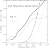 |
Fig. 3 Temperature and velocity profiles from the MUS-b and X-Exo-b models. |
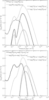 |
Fig. 4 Rates from the MUS-b model. Top: rates of the dominant He(23S) production processes. Bottom: rates of the destruction processes. e− refers to thermal electrons and e* to photoelectrons. |
5 Sensitivity analysis. In-transit spectrum
The preceding analysis confirms the importance of Penning ionization for the loss of the He metastable in He(23S)+H collisions, possibly together with excitation into higher-energy states through He(23S)+e−collisions. It is instructive to compare the simulations based on the rate coefficient for Penning ionization calculated by us (Table A.5), which is consistent with the available experimental and numerical evidence, with simulations based on other prescriptions of the rate coefficient.
The MUS-b-RD82 model is identical to the MUS-b model except that it uses a T-independent rate coefficient of 5 × 10⁻¹⁰ cm3 s−1 for the total of Penning and associative ionization He(23S)+H→He(11S)+H++e−, →HeH++e−. This is the value quoted by Roberge & Dalgarno (1982), who in turn quoted Fort et al. (1978), Neynaber & Tang (1978), and Morgner & Niehaus (1979). We reviewed the original references to track the significant discrepancy between the Roberge & Dalgarno (1982) rate coefficient and ours. It appears that the cross sections reported in the aforementioned references are generally consistent with the Movre & Meyer (1997) cross sections that we used, and with other cross section determinations such as those of Waibel et al. (1988). Figure 5 elaborates further on the comparison with these and other sources. As a consequence, the moderate differences between cross sections cannot explain the large discrepancy in the rate coefficients. We speculate that the Roberge & Dalgarno (1982) value was determined at very low temperature (our calculations yield ~7 × 10⁻¹⁰ cm3 s−1 at 100 K) or that the authors mistakenly adopted the cross sections for He(23S)+D→ionization from Neynaber & Tang (1978). For Penning ionization of H atoms, the MUS-b-FA98 model adopts the ∝T1/2 law noted earlier. No details are given by Fassia et al. (1998) to motivate this extrapolation law.
Figure 6 presents synthetic in-transit spectra of the He I line at 1.08 μm for the MUS-a, MUS-b, X-Exo-a, X-Exo-b, MUS-b-RD82, and MUS-b-FA98 models of GJ 436 b. They were prepared with routines developed by García Muñoz & Schneider (2019) and expressed in the form of excess absorptions. The line optical properties are from the NIST database (Kramida 2010; Kramida et al. 2018). The figure includes the upper limit on the excess absorption inferred by Masson et al. (2024) from their nondetection of the He I line at GJ 436 b. The strength of the in-transit signal is connected to the capacity of the stellar irradiation to drive a vigorous outflow and, therefore, to the planet’s mass loss rate. We obtain (integrated over a solid angle of 4π) mass loss rates of ~2.3×10¹⁰ g/s for the simulations based on the MUSCLES SED and ~7.4×10⁹ g/s for the simulations based on the X-Exoplanets SED. Taking into account the effect of photoelectrons reduces the mass loss rates by ~5–10%.
The MUS-a and -b spectra are barely distinguishable. Similarly, the X-Exo-a and -b spectra are nearly identical. The reason is that the effects of photoelectrons on He(23S) are confined to atmospheric layers that are too deep and contribute little to the in-transit spectra. In contrast, the He(23S) produced by radiative recombination is formed at higher altitudes and effectively sets the stellar area masked by the He I line during transit. It is difficult to anticipate how general this finding is and whether the He(23S) formed from photoelectron-driven excitation makes a greater difference at other planets. We will test this idea in future work by simulating additional planet-star systems.
The comparison of the MUS-b and X-Exo-b spectra demonstrates the importance of the adopted SED. Whereas the MUS-a and -b spectra are clearly inconsistent with the published nondetections, the X-Exo-a and -b spectra are notably closer to the reported upper limits (Nortmann et al. 2018; Guilluy et al. 2024; Masson et al. 2024). The choice of SED may partly explain the problems encountered by past models in explaining the nondetections for GJ 436 b (Oklopčić & Hirata 2018; Dos Santos et al. 2022; Rumenskikh et al. 2023). Taken at face value, the better match obtained with the X-Exoplanets SED suggests that this may be a closer representation of the true stellar SED. This possibility could in principle be tested only with an empirical representation of the SED.
Lastly, we describe the comparison between the MUS-b, MUS-b-RD82, and MUS-b-FA98 models. The He(23S) peak densities (not shown) differ by a factor of approximately three between the MUS-b-RD82 and MUS-b-FA98 models, somewhat less than the factor of six in the adopted rate coefficients at T=5000 K. The corresponding difference in the excess absorption of the in-transit spectra (Fig. 6) is smaller, but larger than the errors often quoted in this type of measurement. As expected, the predicted in-transit spectrum based on our recommended rate coefficient for Penning ionization of H atoms sits somewhere in between. The comparison clearly conveys that significant biases can be introduced by describing some of the key Ch-C-R processes in ways that are not physically motivated.
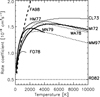 |
Fig. 5 Rate coefficients for total ionization through the processes He(23S)+H→He(11S)+H++e−, →HeH++e−. We calculated these from the (scanned) cross sections reported in the quoted references over a range of temperatures commensurate with the range of energies at which they were reported. The calculations were performed by means of standard expressions and assumed a Maxwellian distribution for the relative velocities between the colliders. Occasionally, we extrapolated the cross sections toward low energies with a ∝E−0.2 law (E is the center-of-mass kinetic energy) and toward high energies with a ∝E−1 law. (References: MI72, Miller et al. (1972); CL73, Cohen & Lane (1973); HM77, Hickman & Morgner (1977); FO78, Fort et al. (1978); MN79, Morgner & Niehaus (1979); WA88, Waibel et al. (1988); MM97, Movre & Meyer (1997)). Also included is the value quoted by Roberge & Dalgarno (1982) and the temperature-dependent expression utilized by Fassia et al. (1998). The expression k [cm3s−1]=10−9 exp(c/T + d1 ln T + d2(ln T)2 + d3(ln T)3) (c=−8.64804E+01; d1=−2.86766E−01; d2=+8.68445E−02; d3=−5.73001E−03) fits the rate coefficient based on the Movre & Meyer (1997) cross sections with errors of <2% from 200 to 10 000 K. |
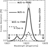 |
Fig. 6 Synthetic in-transit spectra based on the MUS-a, MUS-b, X-Exo-a, X-Exo-b, MUS-b-RD82, and MUS-b-FA98 models. Thin and thick lines refer to -a and -b models, respectively (see text for details). The spectra were calculated following standard methods (García Muñoz & Schneider 2019), with which we obtain the wavelength-dependent effective radius, Rλ. The excess absorption is defined as EA=((Rλ/R⋆)2−(Rp/R⋆)2)×100, with Rp being the planet’s optical radius and R⋆ the stellar radius. Also shown is the nondetection upper limit reported by Masson et al. (2024). Nortmann et al. (2018) and Guilluy et al. (2024) report upper limits of 0.41 and 0.42%, respectively. |
6 Summary
We propose a revised network of chemical-collisional-radiative processes for modeling He(23S) in exoplanet atmospheres. It generalizes past approaches in that it enables the simulation of outflows in which H2 remains undissociated to high altitudes, a valuable addition toward the study of Neptune- and sub-Neptune-sized planets. In our simulations of GJ 436 b, we identify Penning ionization of H atoms as a key process in removing the high-altitude He(23S) that sets the planet’s size at the core of the He I line at 1.08 μm. We calculated the rate coefficient for this process from published cross sections. It differs by factors of a few with respect to other rate coefficient prescriptions found in the literature. A sensitivity analysis shows that the misrepresentation of Penning ionization significantly biases the strength of the He I line at its core. More generally, the misrepresentation of this process may have implications on the He/H2 abundance ratio constrained from observation-model comparisons of other exoplanets.
Large changes in ionization rates driven by photoelectrons do not lead to similarly large changes in the densities of the charged particles. This may be a property of atmospheres in which the background gas remains in molecular form where most of the secondary electrons are released. The idea merits further attention by testing it at other planet-star systems. At GJ 436 b, photoelectron-driven excitation from the He ground state into He(23S) dominates the production of He metastable at p≳10−2 dyn cm−2. However, these layers are too deep to make a difference in the in-transit spectrum. Our finding does not rule out the possibility that photoelectron-driven processes may have a stronger effect in other atmospheres, especially those in which the transition from molecules to atoms occurs in deeper layers.
Lastly, our investigation reveals that the He(23S) population at GJ 436 b is very sensitive to the adopted stellar SED. We tested two SEDs and found that the simulated outflows result in very different in-transit signals. The simulation based on the weakest of the two SED is nearly consistent with the non-detections of the He I line at 1.08 μm from three independent groups.
Data availability
Fits to the rate coefficients can be found via the link.
Acknowledgements
Thanks are due to I. Bray, D. De Fazio, M. Génévriez, J. Loreau, S. Nahar and X. Urbain for feedback on different aspects of the collisional-radiative processes in helium. After acceptance and posting of the current manuscript, Dr. Tommi Koskinen has informed me that his group is also revising the helium network, that some of their findings specific to planet HD 209458 b were presented in a poster at the Exoplanets V conference (Leiden, the Netherlands, 2024), and that their final results have been submitted for publication (Taylor et al., in prep.). Since I was not aware of those efforts, it appears that the two revisions of the helium network have been done independently.
Appendix A Helium network
For reference, Tables A.1–A.8 list information that describes the species and Ch-C-R processes specific to helium in our model. In these tables and throughout the paper, we follow the notation XE+Y=X×10+Y. When appropriate, the rate coefficients have been fitted to expressions of the form aTb exp (c/T)Υ(T), with ln ![Mathematical equation: $\[\Upsilon={\sum}_{t=0}^{3} d_{t}(\ln T)^{t}\]$](/articles/aa/full_html/2025/06/aa55145-25/aa55145-25-eq5.png) and where a, b, c and dt are fit coefficients. Only 5 of the 7 fit coefficients are independent. A SI file contains the details of the expressions.
and where a, b, c and dt are fit coefficients. Only 5 of the 7 fit coefficients are independent. A SI file contains the details of the expressions.
Atom model for helium.
Effective rate coefficients αi,eff [cm3s−1] at selected temperatures for radiative recombination, He++e−→He(i)+hν.
Adopted transition probabilities Aji [s−1] between He states.
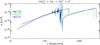 |
Fig. A.1 He photoionization cross sections adopted in the network. From the NORAD database (Nahar 2010, 2020). |
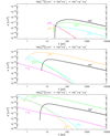 |
Fig. A.2 Excitation, deexcitation and ionization cross sections for collisions of electrons of the specified energies with He atoms. Based on Ralchenko et al. (2008). |
Rate coefficients at selected temperatures for (de)excitation in collisions with thermal electrons, He(i)+e−→He(j)+e−.
Rate coefficients [cm3s−1] at selected temperatures for loss processes of metastable He in collisions with neutrals.
Rate coefficients [cm3s−1] at selected temperatures for some processes involving HeH+.
Rate coefficients [cm3s−1] at selected temperatures for charge exchange.
Photoelectron-driven processes in the network.
References
- Allan, A. P., Vidotto, A. A., Villarreal D’Angelo, C., Dos Santos, L. A., & Driessen, F. A. 2024, MNRAS, 527, 4657 [Google Scholar]
- Ballabio, G., & Owen, J. E. 2025, MNRAS, 537, 1305 [Google Scholar]
- Bean, J. L., Raymond, S. N., & Owen, J. E. 2021, J. Geophys. Res. (Planets), 126, e06639 [NASA ADS] [Google Scholar]
- Ben-Jaffel, L., Ballester, G. E., García Muñoz, A., et al. 2022, Nat. Astron., 6, 141 [NASA ADS] [CrossRef] [Google Scholar]
- Berrington, K. A., & Kingston, A. E. 1987, J. Phys. B At. Mol. Phys., 20, 6631 [NASA ADS] [CrossRef] [Google Scholar]
- Biassoni, F., Caldiroli, A., Gallo, E., et al. 2024, A&A, 682, A115 [NASA ADS] [CrossRef] [EDP Sciences] [Google Scholar]
- Black, J. H. 1978, ApJ, 222, 125 [NASA ADS] [CrossRef] [Google Scholar]
- Bourrier, V., Lecavelier des Etangs, A., Ehrenreich, D., et al. 2018, A&A, 620, A147 [NASA ADS] [CrossRef] [EDP Sciences] [Google Scholar]
- Bray, I., Burgess, A., Fursa, D. V., & Tully, J. A. 2000, A&AS, 146, 481 [NASA ADS] [CrossRef] [EDP Sciences] [Google Scholar]
- Cauley, P. W., Wang, J., Shkolnik, E. L., et al. 2021, AJ, 161, 152 [Google Scholar]
- Cecchi-Pestellini, C., Ciaravella, A., Micela, G., & Penz, T. 2009, A&A, 496, 863 [NASA ADS] [CrossRef] [EDP Sciences] [Google Scholar]
- Cohen, J. S., & Lane, N. F. 1973, J. Phys. B At. Mol. Phys., 6, L113 [Google Scholar]
- Cohen, J. S., & Lane, N. F. 1977, J. Chem. Phys., 66, 586 [Google Scholar]
- Courtney, E. D. S., Forrey, R. C., McArdle, R. T., Stancil, P. C., & Babb, J. F. 2021, ApJ, 919, 70 [Google Scholar]
- Czesla, S., Lampón, M., Sanz-Forcada, J., et al. 2022, A&A, 657, A6 [NASA ADS] [CrossRef] [EDP Sciences] [Google Scholar]
- De Fazio, D. 2014, Phys. Chem. Chem. Phys. (Incorp. Faraday Trans.), 16, 11662 [Google Scholar]
- Dos Santos, L. A., Vidotto, A. A., Vissapragada, S., et al. 2022, A&A, 659, A62 [NASA ADS] [CrossRef] [EDP Sciences] [Google Scholar]
- Drake, G. W. F. 1986, Phys. Rev. A, 34, 2871 [NASA ADS] [CrossRef] [Google Scholar]
- Ehrenreich, D., Bourrier, V., Wheatley, P. J., et al. 2015, Nature, 522, 459 [Google Scholar]
- Fassia, A., Meikle, W. P. S., Geballe, T. R., et al. 1998, MNRAS, 299, 150 [Google Scholar]
- Florescu-Mitchell, A. I., & Mitchell, J. B. A. 2006, Phys. Rep., 430, 277 [Google Scholar]
- Fort, J., Laucagne, J. J., Pesnelle, A., & Watel, G. 1978, Phys. Rev. A, 18, 2063 [Google Scholar]
- Fossati, L., Pillitteri, I., Shaikhislamov, I. F., et al. 2023, A&A, 673, A37 [NASA ADS] [CrossRef] [EDP Sciences] [Google Scholar]
- France, K., Loyd, R. O. P., Youngblood, A., et al. 2016, ApJ, 820, 89 [NASA ADS] [CrossRef] [Google Scholar]
- García Muñoz, A. 2007, Planet. Space Sci., 55, 1426 [Google Scholar]
- García Muñoz, A. 2023a, Icarus, 392, 115373 [CrossRef] [Google Scholar]
- García Muñoz, A. 2023b, A&A, 672, A77 [NASA ADS] [CrossRef] [EDP Sciences] [Google Scholar]
- García Muñoz, A., & Bataille, E. 2024, ACS Earth Space Chem., 8, 2652 [Google Scholar]
- García Muñoz, A., & Schneider, P. C. 2019, ApJ, 884, L43 [Google Scholar]
- García Muñoz, A., Fossati, L., Youngblood, A., et al. 2021, ApJ, 907, L36 [Google Scholar]
- Génévriez, M., Jureta, J. J., Defrance, P., & Urbain, X. 2017, Phys. Rev. A, 96, 010701 [Google Scholar]
- Gillet, A., García Muñoz, A., & Strugarek, A. 2023, A&A, 680, A33 [NASA ADS] [CrossRef] [EDP Sciences] [Google Scholar]
- Gillet, A., Strugarek, A., & García Muñoz, A. 2025, A&A, 696, A64 [NASA ADS] [CrossRef] [EDP Sciences] [Google Scholar]
- Grasser, N., Snellen, I. A. G., Landman, R., Picos, D. G., & Gandhi, S. 2024, A&A, 688, A191 [NASA ADS] [CrossRef] [EDP Sciences] [Google Scholar]
- Guilluy, G., D’Arpa, M. C., Bonomo, A. S., et al. 2024, A&A, 686, A83 [NASA ADS] [CrossRef] [EDP Sciences] [Google Scholar]
- Hickman, A. P., & Morgner, H. 1977, J. Chem. Phys., 67, 5484 [Google Scholar]
- Knutson, H. A., Benneke, B., Deming, D., & Homeier, D. 2014, Nature, 505, 66 [Google Scholar]
- Kramida, A. 2010, Atomic Energy Levels and Spectra Bibliographic Database, version 2.0 (Gaithersburg, MD: NIST) [Google Scholar]
- Kramida, A. & Ralchenko, Y. 2018, NIST Atomid Spectra Database, version 5.5.6 (Gaithesburg, MD: NIST), https://physics.nist.gov/asd [Google Scholar]
- Kulow, J. R., France, K., Linsky, J., & Loyd, R. O. P. 2014, ApJ, 786, 132 [Google Scholar]
- Lampón, M., López-Puertas, M., Sanz-Forcada, J., et al. 2023, A&A, 673, A140 [NASA ADS] [CrossRef] [EDP Sciences] [Google Scholar]
- Locci, D., Aresu, G., Petralia, A., et al. 2024, Planet. Sci. J., 5, 58 [Google Scholar]
- Loreau, J., Ryabchenko, S., Muñoz Burgos, J. M., & Vaeck, N. 2018, J. Phys. B At. Mol. Phys., 51, 085205 [Google Scholar]
- Madhusudhan, N., & Seager, S. 2011, ApJ, 729, 41 [Google Scholar]
- Masson, A., Vinatier, S., Bézard, B., et al. 2024, A&A, 688, A179 [NASA ADS] [CrossRef] [EDP Sciences] [Google Scholar]
- Miller, W. H., Slocomb, C. A., & Schaefer, III, H. F. 1972, J. Chem. Phys., 56, 1347 [Google Scholar]
- Morgner, H., & Niehaus, A. 1979, J. Phys. B At. Mol. Phys., 12, 1805 [Google Scholar]
- Morley, C. V., Knutson, H., Line, M., et al. 2017, AJ, 153, 86 [NASA ADS] [CrossRef] [Google Scholar]
- Moses, J. I., Line, M. R., Visscher, C., et al. 2013, ApJ, 777, 34 [Google Scholar]
- Movre, M., & Meyer, W. 1997, J. Chem. Phys., 106, 7139 [Google Scholar]
- Movre, M., Meyer, W., Merz, A., Ruf, M. W., & Hotop, H. 1994, Chem. Phys. Lett., 230, 276 [Google Scholar]
- Mukherjee, S., Schlawin, E., Bell, T. J., et al. 2025, ApJ, 982, L39 [Google Scholar]
- Nahar, S. N. 2010, New A, 15, 417 [Google Scholar]
- Nahar, S. 2020, Atoms, 8, 68 [NASA ADS] [CrossRef] [Google Scholar]
- Neynaber, R. H., & Tang, S. Y. 1978, J. Chem. Phys., 69, 4851 [Google Scholar]
- Nortmann, L., Pallé, E., Salz, M., et al. 2018, Science, 362, 1388 [Google Scholar]
- Oklopčić, A. 2019, ApJ, 881, 133 [Google Scholar]
- Oklopčić, A., & Hirata, C. M. 2018, ApJ, 855, L11 [Google Scholar]
- Orient, O. J. 1977, Chem. Phys. Lett., 52, 264 [NASA ADS] [CrossRef] [Google Scholar]
- Owen, J. E. 2019, Annu. Rev. Earth Planet. Sci., 47, 67 [CrossRef] [Google Scholar]
- Peacock, S., Barman, T., Shkolnik, E. L., et al. 2019, ApJ, 886, 77 [NASA ADS] [CrossRef] [Google Scholar]
- Preston, R. K., & Cohen, J. S. 1976, J. Chem. Phys., 65, 1589 [Google Scholar]
- Ralchenko, Y., Janev, R. K., Kato, T., et al. 2008, At. Data Nuclear Data Tables, 94, 603 [Google Scholar]
- Roberge, W., & Dalgarno, A. 1982, ApJ, 255, 489 [NASA ADS] [CrossRef] [Google Scholar]
- Rumenskikh, M. S., Khodachenko, M. L., Shaikhislamov, I. F., et al. 2023, MNRAS, 526, 4120 [NASA ADS] [Google Scholar]
- Sanz-Forcada, J., López-Puertas, M., Lampón, M., et al. 2025, A&A, 693, A285 [NASA ADS] [CrossRef] [EDP Sciences] [Google Scholar]
- Schauer, M. M., Jefferts, S. R., Barlow, S. E., & Dunn, G. H. 1989, J. Chem. Phys., 91, 4593 [NASA ADS] [CrossRef] [Google Scholar]
- Schreyer, E., Owen, J. E., Spake, J. J., Bahroloom, Z., & Di Giampasquale, S. 2024, MNRAS, 527, 5117 [Google Scholar]
- Seager, S., & Sasselov, D. D. 2000, ApJ, 537, 916 [Google Scholar]
- Shematovich, V. I., Ionov, D. E., & Lammer, H. 2014, A&A, 571, A94 [NASA ADS] [CrossRef] [EDP Sciences] [Google Scholar]
- Spake, J. J., Sing, D. K., Evans, T. M., et al. 2018, Nature, 557, 68 [Google Scholar]
- Turner, J. D., Christie, D., Arras, P., Johnson, R. E., & Schmidt, C. 2016, MNRAS, 458, 3880 [NASA ADS] [CrossRef] [Google Scholar]
- Vissapragada, S., Knutson, H. A., Greklek-McKeon, M., et al. 2022, AJ, 164, 234 [NASA ADS] [CrossRef] [Google Scholar]
- Waibel, H., Ruf, M. W., & Hotop, H. 1988, Z. Phys. D At. Mol. Clusters, 9, 191 [Google Scholar]
- Wakelam, V., Herbst, E., Loison, J. C., et al. 2012, ApJS, 199, 21 [Google Scholar]
- West, W. P., Cook, T. B., Dunning, F. B., Rundel, R. D., & Stebbings, R. F. 1975, J. Chem. Phys., 63, 1237 [Google Scholar]
- Wiese, W. L., & Fuhr, J. R. 2009, J. Phys. Chem. Ref. Data, 38, 565 [Google Scholar]
- Yan, F., & Henning, T. 2018, Nat. Astron., 2, 714 [Google Scholar]
- Yan, D., Seon, K.-I., Guo, J., Chen, G., & Li, L. 2022, ApJ, 936, 177 [NASA ADS] [CrossRef] [Google Scholar]
- Zygelman, B. 1991, Phys. Rev. A, 43, 575 [Google Scholar]
All Tables
Effective rate coefficients αi,eff [cm3s−1] at selected temperatures for radiative recombination, He++e−→He(i)+hν.
Rate coefficients at selected temperatures for (de)excitation in collisions with thermal electrons, He(i)+e−→He(j)+e−.
Rate coefficients [cm3s−1] at selected temperatures for loss processes of metastable He in collisions with neutrals.
Rate coefficients [cm3s−1] at selected temperatures for some processes involving HeH+.
All Figures
|
Fig. 1 MUSCLES SED (black) and X-Exoplanets SED (gray) at 1 AU and the spectral resolution adopted here. The quoted numbers refer, from left to right, to the integration over the intervals 0→100 Å; 0→503 Å; 0→911 Å; 0→2600 Å, in units of erg cm−2 s−1. |
| In the text | |
|
Fig. 2 Top: production rates of primary (dashed lines) and secondary (dotted lines) electrons from the MUS-a and -b models. Colors separate the contributions by donor. The dashed black line refers to the primaries summed over all donors. The solid black line refers to the total of primaries and secondaries summed over all donors. Bottom: number densities. Dashed and solid lines refer to MUS-a and -b, respectively. Each panel provides, based on the MUS-b model, the conversion between pressure and radial distance normalized to the planet’s optical radius (r/Rp; =1 at the model’s lower boundary). |
| In the text | |
|
Fig. 3 Temperature and velocity profiles from the MUS-b and X-Exo-b models. |
| In the text | |
|
Fig. 4 Rates from the MUS-b model. Top: rates of the dominant He(23S) production processes. Bottom: rates of the destruction processes. e− refers to thermal electrons and e* to photoelectrons. |
| In the text | |
|
Fig. 5 Rate coefficients for total ionization through the processes He(23S)+H→He(11S)+H++e−, →HeH++e−. We calculated these from the (scanned) cross sections reported in the quoted references over a range of temperatures commensurate with the range of energies at which they were reported. The calculations were performed by means of standard expressions and assumed a Maxwellian distribution for the relative velocities between the colliders. Occasionally, we extrapolated the cross sections toward low energies with a ∝E−0.2 law (E is the center-of-mass kinetic energy) and toward high energies with a ∝E−1 law. (References: MI72, Miller et al. (1972); CL73, Cohen & Lane (1973); HM77, Hickman & Morgner (1977); FO78, Fort et al. (1978); MN79, Morgner & Niehaus (1979); WA88, Waibel et al. (1988); MM97, Movre & Meyer (1997)). Also included is the value quoted by Roberge & Dalgarno (1982) and the temperature-dependent expression utilized by Fassia et al. (1998). The expression k [cm3s−1]=10−9 exp(c/T + d1 ln T + d2(ln T)2 + d3(ln T)3) (c=−8.64804E+01; d1=−2.86766E−01; d2=+8.68445E−02; d3=−5.73001E−03) fits the rate coefficient based on the Movre & Meyer (1997) cross sections with errors of <2% from 200 to 10 000 K. |
| In the text | |
|
Fig. 6 Synthetic in-transit spectra based on the MUS-a, MUS-b, X-Exo-a, X-Exo-b, MUS-b-RD82, and MUS-b-FA98 models. Thin and thick lines refer to -a and -b models, respectively (see text for details). The spectra were calculated following standard methods (García Muñoz & Schneider 2019), with which we obtain the wavelength-dependent effective radius, Rλ. The excess absorption is defined as EA=((Rλ/R⋆)2−(Rp/R⋆)2)×100, with Rp being the planet’s optical radius and R⋆ the stellar radius. Also shown is the nondetection upper limit reported by Masson et al. (2024). Nortmann et al. (2018) and Guilluy et al. (2024) report upper limits of 0.41 and 0.42%, respectively. |
| In the text | |
|
Fig. A.1 He photoionization cross sections adopted in the network. From the NORAD database (Nahar 2010, 2020). |
| In the text | |
|
Fig. A.2 Excitation, deexcitation and ionization cross sections for collisions of electrons of the specified energies with He atoms. Based on Ralchenko et al. (2008). |
| In the text | |
Current usage metrics show cumulative count of Article Views (full-text article views including HTML views, PDF and ePub downloads, according to the available data) and Abstracts Views on Vision4Press platform.
Data correspond to usage on the plateform after 2015. The current usage metrics is available 48-96 hours after online publication and is updated daily on week days.
Initial download of the metrics may take a while.