© The Authors 2025

1. Introduction

Modified Newtonian dynamics (MoND) was introduced by Milgrom (1983). It is a non-relativistic modification of the Newtonian law of gravity, which can largely explain the dynamics in galaxies without the need to introduce dark matter. This constitutes an important research program (Merritt 2020) given the tensions between observations and dark-matter-based models (Kroupa et al. 2023). Still, the acceleration, a₀, known as Milgrom's constant needs to be introduced in the theory and must be obtained from data. The value a₀=(1.20±0.02)×10⁻¹⁰ m s⁻² (Lelli et al. 2017) is used for data analysis in Chapter 3. MoND replicates Newtonian behaviour for large gravitational accelerations of a≫a₀, while postulating a logarithmic potential for a≪a₀, recently verified through weak lensing by Mistele et al. (2024). If the gravitational acceleration predicted by MoND is plotted against the gravitational acceleration predicted by Newton's law of gravity, g_N, a deviation from the line of identity for a<a₀ is obtained, so that a>g_N. The functional relation, a(g_N), is called the radial acceleration relation (RAR). The velocity dispersions of many dwarf spheroidal satellite galaxies (dSphs) and galaxy clusters have been reported to be in tension with the RAR (Safarzadeh & Loeb 2021; Lelli et al. 2017; Sánchez-Salcedo & Hernandez 2007; Angus 2008; McGaugh & Milgrom 2013a, b; Alexander et al. 2017). This tension can be interpreted as implying that MoND might not be a generally valid effective description of non-relativistic gravitation. However, this tension needs to be seen in view of the multiple flavours of dSphs among the data of Lelli et al. (2017) and Safarzadeh & Loeb (2021): those that lie along the RAR, those that should not be on the RAR in MoND due to the external field effect (EFE, predicted by MoND), those that are subject to tidal disruption (a relevant process also in Newtonian dynamics, as was shown by Kroupa 1997 and applied to dSph data by McGaugh & Wolf 2010), and those that might be genuinely offset. The dSphs that fall on the RAR generally (though not always) have the best data and those that are offset have consistently less reliable data. In MoND, one must distinguish between isolated dSphs and those subject to the EFE. The former should follow the RAR but the latter should not. Both of these situations assume dynamical equilibrium, but there is a narrow window in which that holds before the EFE becomes tidally disruptive. Judging from the simulations by Brada & Milgrom (2000), some dSphs should be out of equilibrium and off the RAR (Kroupa 1997). The complexity of the gravitational stellar-dynamics allows for new ansatzes (Sanders 2021; McGaugh et al. 2021). Here, we show that generalizing gravitation in the regime of a<a₀ with the help of the p-Laplacian permits a comprehensive accommodation of dSphs and galaxy clusters.

The generalized Poisson equation (GPE) reads (Evans 1982):

$$\nabla ·\left({\left(\frac{\left|\nabla \mathrm{\Phi }(x)\right|}{a_0}\right)}^{p-2}\nabla \mathrm{\Phi }(x)\right)=4\pi G\rho (x).$$(1)

Φ(x) is the gravitational potential, such that the acceleration is a(x) = −∇Φ with a=|a|. G is the gravitational constant, ρ(x) the mass density distribution, and x the position vector. p is a real dimensionless parameter with p>1 (Lindqvist 2019a). For p = 2, it follows the Newtonian potential. For p = 3, the logarithmic Milgromian potential is obtained outside of ρ(x). Aside from these two p values, there is no physical meaning of p known in the context of gravitational theory. The data analysed here allows for the possibility that the p-Laplacian approach combines the non-equilibrium dynamics (EFE and tidal disruption) through a varying p value. In electrodynamics, the p-Laplacian with arbitrary p is used to describe electrorheological fluids, which are a special sort of non-linear dielectrics (Růžička 2000). There, p is a material constant and can be a function of the electric field. Interpreting p as the dimension of three-dimensional or higher-dimensional Euclidean space, Milgrom (1997) showed the GPE to be conformally invariant. The analysis presented here does not follow his interpretation, but investigates a functional relation between p and ρ(x), assuming ρ(x) to be isolated, and a possible functional relation between p and an external Newtonian gravitational field, g_tot. This analysis considers simple solutions for arbitrary p in spherical symmetry in Sect. 2, applies them to data on dSphs and galaxy clusters in Sect. 3, elaborates on MoND being possibly not fundamental dynamics in Sect. 4, and discusses possible physical implications in Sect. 5.

2. Derivation of the RAR, gravitational potential, and velocity dispersion assuming Plummer models for arbitrary p

2.1. RAR

In this subsection, the RAR is derived for arbitrary p from the GPE, Eq. (1), as a static spherically symmetric problem. This generalized RAR enables to obtain the p parameters in Sect. 3. The GPE simplifies in spherical symmetry with $a(r):=\left|{\partial }_r\mathrm{\Phi }\right|$ to the expression

$$\frac{1}{r^2}{\partial }_r\left(r^2{\left(\frac{a(r)}{a_0}\right)}^{p-2}a(r)\right)=4\pi G\rho (r).$$(2)

The Newtonian acceleration, g_N(r), at a distance, r, in a spherical volume, $V=\frac{4\pi }{3}{r}^3$, is given by

$$g_{\text{N}}(r)=\frac{\mathit{GM}(r)}{r^2}=\frac{4\pi G}{r^2}{\displaystyle \underset{0}{\overset{r}{\int }}}\rho (r^{\prime }){r^{\prime }}^2\text{d}{r}^{\prime },\hspace{0.5em}\text{with the mass}$$(3)

$$M(r):=4\pi {\displaystyle \underset{0}{\overset{r}{\int }}}\rho (r^{\prime }){r^{\prime }}^2\text{d}{r}^{\prime }.$$(4)

Solving the GPE, Eq. (2) by radial integration leads to the p-dependent relation between the fundamental and Newtonian accelerations:

$$\frac{a(r)}{a_0}=\sqrt[p-1]{\frac{g_{\text{N}}(r)}{a_0}},$$(5)

and is shown in Fig. 1. In the Newtonian case p = 2, the RAR becomes the identity. For large p:

$$\underset{p\to \infty }{lim}a(r)=a_0.$$(6)

Fig. 1. RAR for arbitrary p. The bold grey lines indicate the RARs for different p (Eq. (5)).

Solving Eq. (5) for a(r) yields::

$$a(r)=\sqrt[p-1]{\frac{\mathit{GM}(r)a_0^{p-2}}{r^2}}·$$(7)

In the cases p = 2 and p = 3, Eq. (7) simplifies to the Newtonian and Milgromian gravitational accelerations:

$$p=2\Rightarrow a(r)=\frac{\mathit{GM}(r)}{r^2},$$(8)

$$p=3\Rightarrow a(r)=\frac{\sqrt{\mathit{GM}(r)a_0}}{r}·$$(9)

2.2. The velocity dispersion of the generalized Plummer mass distribution

In this subsection, the velocity dispersion for arbitrary p and a Plummer model is derived. The Plummer model is a simple and proper density distribution to describe dSphs. The velocity dispersion cannot be calculated independently of the density distribution, if p≠3 (for a proof, see Appendix F). We considered the gravitational acceleration for arbitrary p (Eq. (7)) and the Plummer model (p. 81 in Heggie & Hut 2003):

$$M(r)=M_{\text{st}}\frac{{\left(\frac{r}{r_{\text{pl}}}\right)}^3}{{\left(1+{\left(\frac{r}{r_{\text{pl}}}\right)}^2\right)}^{\frac{3}{2}}},$$(10)

$$\rho (r)=\frac{3M_{\text{st}}}{4\pi r_{\text{pl}}^3}\frac{1}{{\left(1+{\left(\frac{r}{r_{\text{pl}}}\right)}^2\right)}^{\frac{5}{2}}},$$(11)

with the Plummer radius, r_pl, and stellar mass, M_st. The radial component of the isotropic velocity dispersion, ${\sigma }_r^2(r)$, obtained from the Jeans equation, reads (Chap. 4.8 in Binney & Tremaine 2008):

$${\sigma }_r^2(r)=\frac{1}{\rho (r)}{\displaystyle {\int }_r^{\infty }}\rho (r^{\prime })a(r^{\prime })\text{d}{r}^{\prime }.$$(12)

Inserting Eqs. (7), (10) and (11) into Eq. (12) yields:

$${\sigma }_r^2(r)=C(p){\left(1+{\left(\frac{r}{r_{\text{pl}}}\right)}^2\right)}^{\frac{5}{2}}{\displaystyle \underset{r}{\overset{\infty }{\int }}}\frac{1}{{\left(1+{\left(\frac{r^{\prime }}{r_{\text{pl}}}\right)}^2\right)}^{\frac{5}{2}}}{\left(\frac{\frac{r^{\prime }}{r_{\text{pl}}}}{{\left(1+{\left(\frac{r^{\prime }}{r_{\text{pl}}}\right)}^2\right)}^{\frac{3}{2}}}\right)}^{\frac{1}{p-1}}{r}_{\text{pl}}^{\frac{-2}{p-1}}\text{d}{r}^{\prime }$$(13)

$$=C(p){\left(1+{\left(\frac{r}{r_{\text{pl}}}\right)}^2\right)}^{\frac{5}{2}}{r}_{\text{pl}}^{\frac{p-3}{p-1}}{\displaystyle \underset{q(r)}{\overset{\infty }{\int }}}{\left(\frac{q(r^{\prime })}{(1+q(r^{\prime }{)}^2{)}^{\frac{5p-2}{2}}}\right)}^{\frac{1}{p-1}}\text{d}q(r^{\prime })$$(14)

$$=\frac{p-1}{p}C(p){\left(1+{\left(\frac{r}{r_{\text{pl}}}\right)}^2\right)}^{\frac{5}{2}}{r}_{\text{pl}}^{\frac{p-3}{p-1}}(\underset{q(r)\to \infty }{lim}I(q(r),p)-I(q(r),p)),$$(15)

after introducing the following definitions:

$$q(r):=\frac{r}{r_{\text{pl}}},$$(16)

$$C(p):=\sqrt[p-1]{{\mathit{GM}}_{\text{st}}{a}_0^{p-2}},$$(17)

$$I(q,p):=q^{\frac{p}{p-1}}{}_2{F}_1\left(\frac{2-5p}{2-2p},\frac{p}{2p-2};\frac{3p-2}{2p-2};-q^2\right),$$(18)

where ₂F₁(a,b;c;z) is the hypergeometric function.

The characteristic 1D velocity dispersion, ${\sigma }_{1\mathrm{D}}^2:=\frac{2}{3}\frac{K}{M_{\text{st}}}$, was obtained. $K:=\frac{3}{2}\underset{0}{\overset{\infty }{\int }}{\sigma }_r^2(r)\rho (r)4\pi r^2\text{d}r$ is the kinetic energy (Chap. 4.8 in Binney & Tremaine 2008) for the Plummer sphere.

$${\sigma }_{1\mathrm{D}}^2=\frac{1}{M_{\text{st}}}{\displaystyle \underset{0}{\overset{\infty }{\int }}}{\sigma }_r^2(r)\rho (r)4\pi r^2\text{d}r.$$(19)

Inserting Eq. (15) for σ_r(r) and Eq. (11) for ρ(r) yields:

$${\sigma }_{1\mathrm{D}}^2=3\mathrm{\Omega }(p)r_{\text{pl}}^{-3}·{\displaystyle \underset{0}{\overset{\infty }{\int }}}\mathrm{\Lambda }(q(r),p)r^2\text{d}r,$$(20)

with

$$\mathrm{\Omega }(p):=\frac{p-1}{p}·C(p)·r_{\text{pl}}^{\frac{p-3}{p-1}},$$(21)

$$\mathrm{\Lambda }(q(r),p):=\left(\underset{q(r)\to \infty }{lim}I(q(r),p)-I(q(r),p)\right).$$(22)

Converting the integration variable to q(r) and integrating by parts results in:

$${\sigma }_{1\mathrm{D}}^2=\mathrm{\Omega }(p)·([q(r{)}^3\mathrm{\Lambda }(q(r),p){]}_{q(r)=0}^{q(r)\to \infty }$$(23)

$$-{\displaystyle \underset{0}{\overset{\infty }{\int }}}q(r{)}^3{\partial }_{q(r)}\mathrm{\Lambda }(q(r),p)\text{d}q(r))$$(24)

$$=\mathrm{\Omega }(p)·([q(r{)}^3\mathrm{\Lambda }(q(r),p){]}_{q(r)=0}^{q(r)\to \infty }$$(25)

$$+\frac{p}{p-1}·{\displaystyle \underset{0}{\overset{\infty }{\int }}}q(r{)}^3{\left(\frac{q(r)}{(1+q(r{)}^2{)}^{\frac{5p-2}{2}}}\right)}^{\frac{1}{p-1}}\text{d}q(r))$$(26)

$$=\mathrm{\Omega }(p)·\underset{q\to \infty }{lim}\left(q^3\mathrm{\Lambda }(q,p)+I^{\prime }(q,p)\right),$$(27)

with

$$I^{\prime }(q,p):=\frac{p}{4p-3}{q}^{\frac{4p-3}{p-1}}{}_2{F}_1\left(\frac{2-5p}{2-2p},\frac{3-4p}{2-2p};\frac{5-6p}{2-2p};-q^2\right).$$(28)

In the last step, the lower limit q(r) of the integral (Eq. (20)) does not contribute: for p>1, lim_q→0(Λ(q,p)) is finite, lim_q→0(q³) = 0, ${lim}_{q\to 0}(q^{\frac{4p-3}{p-1}})=0$, and ${}_2{F}_1(\frac{2-5p}{2-2p},\frac{3-4p}{2-2p};\frac{5-6p}{2-2p};0)=1$. Using l’H$\hat{\text{o}}$spital's rule for

$$\underset{q\to \infty }{lim}\frac{\mathrm{\Lambda }(q,p)}{q^{-3}}=\underset{q\to \infty }{lim}\frac{{\partial }_q\mathrm{\Lambda }(q,p)}{-3q^{-4}}=\underset{q\to \infty }{lim}{q}^{\frac{-5p-1}{p-1}}=0,\text{if}\hspace{0.5em}p>1,$$(29)

leads to the final expression for ${\sigma }_{1\mathrm{D}}^2$:

$${\sigma }_{1\mathrm{D}}^2=\mathrm{\Omega }(p)·\underset{q\to \infty }{lim}{I}^{\prime }(q,p).$$(30)

In Sect. 3, velocity dispersions for dSphs are calculated with Eq. (30). The Plummer model requires spherical symmetry and the velocity distribution is assumed to be isotropic. In general, this is not likely to be true for dSphs (Kroupa 1997).

2.3. Newtonian (p = 2) and Milgromian (p = 3) limit for the velocity dispersion

In the Newtonian (p = 2) and Milgromian (p = 3) limit, Eq. (30) reduces to the known expressions for the 1D velocity dispersion (cf. Binney & Tremaine 2008 and Milgrom 1994):

$$p=2\Rightarrow {\sigma }_{1\mathrm{D}}^2=\frac{\pi }{32}\frac{{\mathit{GM}}_{\text{st}}}{r_{\text{pl}}},$$(31)

$$p=3\Rightarrow {\sigma }_{1\mathrm{D}}^2=\frac{2}{9}\sqrt{a_0{\mathit{GM}}_{\text{st}}}.$$(32)

This result for p = 3 is only valid in the field limit for a one-dimensional component of isotropic velocity dispersion. Also, it can be derived from other principles, such as scale invariance in the modified-gravity framework (Milgrom 2014).

3. Data analysis

The data of Milky Way and Andromeda satellite dSphs from Lelli et al. (2017) and a selection from the HIghest X-ray FLUx Galaxy Cluster Sample (HIFLUGS) from Li et al. (2023) were used to check whether they hint at a relation between p and the density of the satellite galaxy or the galaxy cluster. To accomplish this, what we interpret to be g_N and a from observations was obtained for each dSph and galaxy cluster. Since there is no interest in the radial dependence of g_N(r) and a(r), from now on g_N and a is written. With the RAR for arbitrary p derived in Chapter 2, p was calculated. From these p parameters, velocity dispersions were obtained for the Milky Way dSphs analysed. All relevant data are shown in Table A.1 for the dSphs and in Table B.1 for the galaxy clusters. Figure 2 shows the data compared to the RAR for arbitrary p derived in Chapter 2.

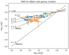Fig. 2. RAR for selected Milky Way (blue) and Andromeda (orange) satellite dSphs and galaxy clusters (green). Uncertainties are 1σ. The data are taken from Lelli et al. (2017) for the dSphs (Milky Way and Andromeda satellites) and Li et al. (2023) for the galaxy clusters, as is tabulated in Tables A.1 and B.1, respectively. The bold grey lines for different p are the same as in Fig. 1.

For error propagation, normally distributed and uncorrelated values were assumed. The error Δα of an arbitrary quantity α(β₁,…,β_n) was calculated from arbitrary quantities, β₁,…,β_n, $n\in \mathbb{N}$, with uncertainties of Δβ₁,…,Δβ_n:

$$\mathrm{\Delta }\alpha =\sqrt{{\displaystyle \sum _{i=1}^n}{\left(\frac{\partial \alpha }{\partial {\beta }_i}\mathrm{\Delta }{\beta }_i\right)}^2}.$$(33)

Uncertainties were calculated to two significant digits. If the third significant digit was smaller than 5, uncertainties were rounded down; otherwise, they were rounded up.

3.1. RAR for the data at hand

What we interpret to be g_N and a of the dSphs has been inferred by Lelli et al. (2017) from observational quantities. To accomplish this, they collected distances, V-band magnitudes, half-light-radii, and velocity dispersions from various sources. Velocity dispersions were obtained from high-resolution individual-star spectroscopy. We adopted their values, interpreting their data in the following way:

$$g_{\text{N}}=g_{\text{bar}},$$(34)

$$a=g_{\text{obs}}.$$(35)

They calculated g_bar with Newton's law of gravity and stellar mass, only contributing and g_obs from velocity dispersion using an estimator by Wolf et al. (2010). Here, the analysis was limited to their high-quality sample, reducing the impact of tidal effects and neglecting galaxies with ellipticity larger than 0.45 (for details, see Lelli et al. 2017).

From the HIFLUGS clusters, the gas mass, M_gas,500, stellar mass, M_*,500, and dynamical mass, M_dyn,500, within the virial radius, r₅₀₀, were used. Li et al. (2023) obtained the gas mass from integrating surface brightness fits and the gas mass by assuming a correlation to the stellar mass. They inferred the dynamical mass from X-ray and optical data, taking into account various morphological properties, dynamical properties, and the temperature, assuming hydrostatic equilibrium. They took their values for the virial radius from Zhang et al. (2011), who obtained it from the X-ray measured mass distribution, assuming hydrostatic equilibrium.

The same derivation as in Li et al. (2023) was followed here. From the gas mass, M_gas,500, stellar mass, M_*,500, and dynamical mass, M_dyn,500, enclosed in the virial radius, r₅₀₀, for the galaxy clusters (gc), a and g_N were computed according to Newton's law of gravity:

$$g_{\mathrm{N},\mathrm{gc}}=G·\frac{M_{\text{gas},500}+M_{*,500}}{r_{500}^2},$$(36)

$$a_{\text{gc}}=G·\frac{M_{\text{dyn},500}}{r_{500}^2},$$(37)

with the gravitational constant G=(4.300 917 270 6±0.0000000003) pc/M_⊙(km s)². Uncertainties were not given explicitly by Li et al. (2023). Uncertainties were taken for M_gas,500 from Zhang et al. (2011) and calculated for M_*,500 according to Eq. (23) in Li et al. (2023):

$$\mathrm{\Delta }{M}_{*,500}=\frac{4}{95}·{\left(\frac{5.7\times {10}^{13}{\mathrm{M}}_{\odot }}{M_{\text{gas},500}}\right)}^{0.4}·\mathrm{\Delta }{M}_{\text{gas},500}.$$(38)

Uncertainties were not reconstructed for r₅₀₀ and M_dyn,500, and so underestimated the uncertainties for g_N and a. The uncertainty from the gravitational constant, G, was neglected, since it is so small that it would not contribute significantly to the uncertainties for g_N and a.

Figure 2 shows the RAR for the data at hand. Deviations from the p = 3 line can clearly be seen. For Canes Venatici I, the deviation reaches a 5σ significance. The galaxy cluster data show a 5σ deviation at least from the p = 3 limit, subject to the caveat that their uncertainties are underestimated.

3.2. Calculating p from the RAR and density for the data at hand

To calculate p for the data at hand, Eq. (5) was used. Solving Eq. (5) for p yields:

$$p=\frac{{log}_{10}\left(\frac{g_{\text{N}}}{a_0}\right)}{{log}_{10}\left(\frac{a}{a_0}\right)}+1.$$(39)

Error propagation according to Eq. (33) demands symmetrical uncertainties, which is not fulfilled the values for a and g_N. Uncertainties are therefore symmetrized by taking the larger uncertainty, overestimating the uncertainties. The error of a₀ does not significantly influence the uncertainties of p for the dSphs, but for galaxy clusters. This is because not all relevant uncertainties for the galaxy clusters are considered. The baryonic mass of the dSphs was computed from their V-band luminosity, L_V, and the stellar mass-to-light-ratio, ${\mathrm{\Upsilon }}_{*}=(2.0\pm 0.5){\mathrm{M}}_{\odot }{\mathrm{L}}_{\odot }^{-1}$, given by Lelli et al. (2017):

$$M_{\text{dSphs}}={\mathrm{\Upsilon }}_{*}·L_{\text{V}}.$$(40)

Lelli et al. (2017) inferred the mass-to-light-ratio as a statistical mean from studies of Fornax and Sculptor dSphs by de Boer et al. (2012). The mean density, ${\overline{\rho }}_{\text{dSphs}}$, of the dSphs was estimated from their half-light-radius, r_1/2, from Lelli et al. (2017):

$${\overline{\rho }}_{\text{dSphs}}=\frac{4\pi }{3}·\frac{M_{\text{dSphs}}}{2r_{1/2}^3}·$$(41)

The mean density, ${\overline{\rho }}_{\text{gc}}$, of the galaxy clusters was estimated as:

$${\overline{\rho }}_{\text{gc}}=\frac{4\pi }{3}·\frac{M_{\text{gas},500}+M_{*,500}}{r_{500}^3}·$$(42)

The exact shape was considered for neither the dSphs nor the galaxy clusters, which leads to a systematic uncertainty.

Figure 3 shows the density of the analysed dSphs and galaxy clusters against p. The p parameters deviate from p = 3, in many cases with a 1σ significance, in some with a 2σ significance, and for Canes Venatici I with a 5σ significance. The uncertainties on L_V and r_1/2, and therefore on p of Canes Venatici I, are relatively small. For the galaxy clusters, we refrained from making a claim, since the uncertainties were underestimated. Furthermore, the Python package kafe2 was used to fit an exponential function of the following form and with the parameters ρ_α and α to the data, with ndf being the number of degrees of freedom:

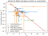Fig. 3. Relation between density of dSphs (blue and orange) and galaxy clusters (green) and p parameter from GPE, Eq. (1). Uncertainties are 1σ. p was obtained from the RAR, as is shown in Fig. 2. See Tables A.1 and B.1 for values. The red line is an exponential function fit to the data with χ2/ndf = 8.001.

$$\rho (p)={\rho }_{\alpha }·exp(\alpha ·p)\hspace{0.5em},$$(43)

$${\rho }_{\alpha }=(54\pm 19){\mathrm{M}}_{\odot }{\mathrm{pc}}^{-3},$$(44)

$$\alpha =(-1.614\pm 0.043),$$(45)

$${\chi }^2/\text{ndf}=8.001,$$(46)

$$\text{ndf}=43.$$(47)

8 M_⊙ pc⁻³ was used as a starting value for ρ_α. The large χ²/ndf was due to the small uncertainties for the galaxy clusters that were underestimated. Without the galaxy clusters, χ²/ndf = 3.115 is obtained¹. This behaviour is extrapolated to the critical density, ρ_crit, of the Universe at redshift z = 0 from the WMAP 7-year cosmology implemented in the astropy.cosmology Python package:

$${\rho }_{\text{crit}}\approx 1.38\times {10}^{-7}{\mathrm{M}}_{\odot }{\mathrm{pc}}^{-3},$$(48)

$$p({\rho }_{\text{crit}})=12.27\pm 0.39.$$(49)

3.3. Infinity Laplacian for weak fields

When p→∞, the p-Laplace operator transitions to a limiting form. The non-linear operator, $-\nabla ·\left(|\nabla \varphi {|}^{p-2}\nabla \varphi \right)$, tends to the infinity Laplacian (Lindqvist 2015):

$${\mathrm{\Delta }}_{\infty }\varphi =\nabla \varphi ·\nabla \left(\nabla \varphi \right)={\displaystyle {\sum }_{i,j}}\frac{\partial \varphi }{\partial x_i}\frac{{\partial }^2\varphi }{\partial x_i\partial x_j}\frac{\partial \varphi }{\partial x_j},$$(50)

where ∇(∇ϕ) represents the Hessian matrix of second derivatives, and the shorthand ∇ϕ·∇(∇ϕ) is equivalent to ∇ϕ^⊤(∇²ϕ)∇ϕ. The indices i and j range over the three spatial dimensions, and ∂ denotes partial differentiation. The infinity Laplacian governs the minimization of the maximum gradient magnitude of the potential, ϕ, a problem known as the absolutely minimal Lipschitz extension problem (Camilli et al. 2017). Lu & Wang (2008) prove that when the infinity Laplacian is applied to a positive source function, Δ_∞ϕ=f(x), and when this function tends to zero, the infinity Laplace operator suppresses variations in the magnitude of ∇ϕ (Lu & Wang 2008, see their Theorem 3.1). Consequently, the inhomogeneous infinity Laplacian converges to the homogeneous case, i.e., Δ_∞ϕ = 0. In the case of matter, the source function is always f(x)≥0. This limiting equation implies that the infinity-Laplace operator smooths out the steepest gradients (Lindqvist 2019b), yielding a gravitational acceleration field with nearly constant magnitude, as anticipated in Eq. (9). This result independently shows that in the weakest gravitational potentials, the GPE predicts that gravity smooths out any sharp variations of the gradient magnitude across the non-linear domain.

3.4. Limitations of this analysis

The present work serves as an invitation for future observational studies, which are within reach instrumentally but which have yet to undergo systematic and thorough investigation. To reduce the uncertainty for the mass-to-light-ratios of the dSphs, we suggest an analysis that considers individual mass-to-light-ratios for the dSphs. This could be achieved within a homogeneous study by one single team. In such an analysis, uncertainties on a and g_N might also be reduced. To estimate the density more accurately, we suggest considering the shape of the individual objects analysed. That the half-light-radius is used for the dSphs and the virial radius for the galaxy clusters might complicate comparability. We also suggest in the future an analysis with all uncertainties for the galaxy clusters. These improvements have not been possible here as the corresponding data are not available.

Finally, the present work constitutes a static analysis of the dynamics generated by the GPE, Eq. (1). At present, live simulations of the studied objects are only possible for the p = 2 and p = 3 cases (e.g. using the code Phantom of Ramses, Lüghausen et al. 2015). Simulations of the satellite galaxies orbiting their host galaxy can thus be performed for these values of p. For example, a detailed study for p = 2 by Kroupa (1997) already suggested that even Newtonian solutions without dark matter exist for most of the galaxy's satellites. It will be important to extend such work to the p = 3 case to study if apparent p>3 solutions emerge.

3.5. Calculating the velocity dispersion for the Plummer model from an obtained p

To infer velocity dispersions of the dSphs from the data by Lelli et al. (2017), Eq. (30) was used, identifying $r_{\text{pl}}=\frac{r_{1/2}}{1.305}$ (Kroupa 2008) and M_st=M_dSphs. Now, the full sample of Milky Way satellites was used and compared to the Lelli et al. (2017) and Safarzadeh & Loeb (2021) data neglecting errors in Fig. 4. The sample of Milky Way satellites chosen by Safarzadeh & Loeb (2021) was used. The latter adopted velocity dispersion data from various astrophysical literature sources. Any calculated velocity dispersion lies within the 1σ regime of the corresponding data point by Lelli et al. (2017) and often also of the corresponding Safarzadeh & Loeb (2021) point. The outliers are Ursa Minor with a 2σ tension and Bootes I as well as Fornax with a 3σ tension between the Lelli et al. (2017) and Safarzadeh & Loeb (2021) points. The ellipticity of Ursa Minor is 0.54, which might not be negligible. Still, for Ursa Major I with an ellipticity of 0.80, there is no tension at all. Bootes I has no peculiar properties; there might be a systematic uncertainty that has not been considered. Fornax is the most massive Milky Way dSph in the sample at hand.

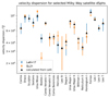Fig. 4. 1D velocity dispersion for selected Milky Way satellite dSphs. Blue are data by Lelli et al. (2017) and orange data by Safarzadeh & Loeb (2021). The black triangles were calculated from the Lelli et al. (2017) data with Eq. (30).

4. Interpreting GPE as a modification of gravitational acceleration under the influence of external Newtonian gravity

In this section, the following hypothesis is examined: the GPE and MoND are not a modification of fundamental dynamics, but just a modification of acceleration. Drawing an analogy to electrorheological fluids suggests that gravity remains Newtonian on a fundamental level, but the p parameter describes a non-linear response of the ‘induced’ field, a(r), inside the satellite galaxy to an external Newtonian field, g_host(r), by the host galaxy and g_N(r) by the satellite itself. This would mean that the Poisson equation still holds true while the gravitational field is modified:

$$\nabla ·g_{\text{tot}}=4\pi G{\rho }_{\text{tot}}(r),$$(51)

$$g_{\text{tot}}:=g_{\text{host}}(r)+g_{\text{N}}(r)={\left(\frac{|a(r)|}{a_0}\right)}^{p-2}a(r).$$(52)

In this picture, g_tot takes the role of electric field strength, E, and a the role of electric displacement, D. The p parameter is used to describe viscosity behaviour of electrorheological fluids. An analogue physical process in galaxies is unknown. The theory of electrorheological fluids postulates a functional relation between the p parameter and the external field. Here, we likewise inquire whether an analogue relation might exist for the analysed dSphs. For this task, the p parameter is re-evaluated:

$$p=\frac{{log}_{10}\left(\frac{g_{\text{tot}}}{a_0}\right)}{{log}_{10}\left(\frac{a}{a_0}\right)}+1,$$(53)

$$g_{\text{tot}}:=|g_{\text{tot}}|=|g_{\text{N}}+g_{\text{host}}|=g_{\text{N}}+g_{\text{host}},$$(54)

$$g_{\text{host}}:=\frac{{\mathit{GM}}_{\text{host}}}{D_{\text{host}}^2}·$$(55)

Equation (54) holds thanks to superposition and spherical symmetry. M_host is the mass of the host galaxy (M_host = 1×10¹² M_⊙ for the Milky Way and M_host = 2×10¹² M_⊙ for Andromeda). D_host is the distance of the satellite to its host. All values were again taken from Lelli et al. (2017). Since no uncertainties for M_host and D_host were given, the uncertainties for g_tot were the same as for g_N. The uncertainty on G was still neglected. For this task, all 60 satellites analysed by Lelli et al. (2017) were investigated. A logarithmic fit leads to the following result in Fig. 5:

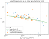Fig. 5. Relation between p parameter and external field gtot for Milky Way (blue) and Andromeda (orange) satellite dSphs. The dashed line describes Milgrom's constant a0. Uncertainties are not shown to keep the plot legible (see Tables C.1 and D.1 for uncertainties on p). The external field is Newtonian and consists of the field by the host galaxy and the internal field of the satellite. A logarithmic fit function (solid green curve) described by Eq. (56) suggests a functional relation, p(gtot).

$$p=p_0·{log}_{10}(\frac{g_{\text{tot}}}{g_0})+1,$$(56)

$$p_0=(-0.74\pm 0.043),$$(57)

$$g_0=(2.0\pm 4.0)\times {10}^{-10}{\mathrm{m}\mathrm{s}}^{-2},$$(58)

$${\chi }^2/\text{ndf}=0.02892,$$(59)

$$\text{ndf}=60.$$(60)

The fit model (Eq. (56)) was chosen to be identical to Eq. (53), if a₀=g₀ and $p_0=\frac{1}{{log}_{10}\left(\frac{a}{a_0}\right)}$. Due to large uncertainties, these identities cannot be confidently defended. This would imply that a∝a₀. Extrapolating to large g_tot is unphysical, since Eq. (56) does not reproduce Newtonian behaviour and allows p≤1, which is mathematically forbidden (Lindqvist 2019a). Still, extrapolating to low accelerations yields a testable prediction. The small χ²/ndf is due to large uncertainties. There seem to be five outliers, including two Milky Way dSphs with p≤1. Still, the uncertainties are so large that they cannot be identified as such.

5. Discussion

This analysis leads to the following conclusions:

1. The gravitational acceleration, a(r), generated by the source distribution can be given by Eq. (7), derived from the GPE, Eq. (1), with p depending on $\overline{\rho }$ according to Eq. (43)².

2. For large p, the Milgromian gravitational acceleration, a, becomes independent of the central mass and distance and equals a₀ (Eq. (6)).

3. The analysed data hint at a relation between p and the density of the bound system, $\overline{\rho }$ (Eq. (43)). The lower the density, the higher p. For the critical density, p(ρ_crit) = 12.27±0.39 is found.

4. Combining the GPE with a Plummer model predicts the observed velocity dispersions in Milky Way dSphs with a less than 1σ deviation without exception (Fig. 4). That is, once the density of the satellite galaxy is known, we can determine the p parameter using Eq. (43), and from Eq. (30) we obtain an estimate for the velocity dispersion.

5. Interpreting the GPE as fundamentally Newtonian, but the gravitational field, a, as a non-linear response to an external field, g_tot, requires a relation, p(g_tot). The analysed data hints at such a relation (Fig. 5).

Items 2 and 3 imply that for densities of the bound system on cosmological scales, the Milgromian gravitational acceleration, a, becomes non-directional and independent of central mass and distance and equals a₀. This increases the gravitational acceleration compared to Newtonian gravity, reducing the need for dark matter. Free particles are not possible for p>3, since ${\displaystyle \underset{r\to \infty }{lim}}\mathrm{\Phi }(r)$ does not exist. The exponential fit (Eq. (43)) cannot be extrapolated to densities related to p<2, because it is known that there is Newtonian gravitation (p = 2) for far larger densities than ρ(p = 2) = (2.14±0.78) M_⊙ pc⁻³.

Items 1 and 2 were derived from the model presented in Sect. 2. This model makes many simplifying assumptions (e.g. spherical symmetry) discussed in Sect. 2. Item 3 is suggested by the data presented in Sect. 3. From the data, claims of up to 5σ significance are stated.

Item 4 might solve the problem of MoND not being able to predict all velocity dispersions in Milky Way satellites raised by Safarzadeh & Loeb (2021). It must be considered that the p parameters have been inferred from the observed accelerations, which have been inferred from velocity dispersions by (Lelli et al. 2017). An independent test might be beneficial to check whether the data correctly represent the Milgromian acceleration, a, which is fundamentally independent of the velocity dispersion.

Apart from items 3 and 5, the physical meaning of p is to be explored. p might be explained by drawing the parallel to electrorheological fluids. This has been done for standard MoND by Blanchet (2007). The data suggests a relation p(g_tot), which makes a prediction for low accelerations. Still, an analysis with more precise data is desirable. If the analogy to electrorheological fluids were justified, any data analysis would always have to explore the effect of external fields. Furthermore, this raises the question of whether there is a physical process leading to a non-linear response of dSphs to external gravitational fields. The analysis presented here may suggest that the GPE describes an effective coupling between the dynamics of a low-acceleration system to the gravitational field in the non-relativistic limit.

This analysis is yet another hint that there might be a deeper underlying gravitational theory generalizing MoNDian and Newtonian gravity. This justifies further reviewing current cosmological models and gravitational theories.

Acknowledgments

We thank the anonymous referee and Mordehai Milgrom for their constructive comments. P.K. acknowledges support from the DAAD-Eastern European exchange programme at the University of Bonn and Charles University in Prague. E.G. acknowledges the support of the National Natural Science Foundation of China (NSFC) under grants NOs. 12173016, 12041305. E.G. acknowledges the science research grants from the China Manned Space Project with NOs. CMS-CSST-2021-A08, CMS-CSST-2021-A07.

References

Appendix A: RAR data

Cluster	$\frac{r_{500}}{\mathrm{kpc}}$	$\frac{M_{\text{gas},500}}{{10}^{13}{\mathrm{M}}_{\odot }}$	$\frac{M_{*,500}}{{10}^{12}{\mathrm{M}}_{\odot }}$	$\frac{M_{\text{dyn},500}}{{10}^{14}{\mathrm{M}}_{\odot }}$	${log}_{10}\left(\frac{g_{\text{N}}}{{\mathrm{m}\mathrm{s}}^{-2}}\right)$	${log}_{10}\left(\frac{a}{{\mathrm{m}\mathrm{s}}^{-2}}\right)$	p	$\frac{\overline{\rho }}{{10}^{-4}{\mathrm{M}}_{\odot }{\mathrm{pc}}^{-3}}$
A0085	1217	6.67(32)	4.39(13)	8.66	-11.175(20)	-10.089	8.46(30)	1.652(74)
A0262	755	1.08(12)	1.47(10)	1.35	-11.523(43)	-10.481	3.858(80)	1.19(12)
A0496	967	2.79(12)	2.60(7)	4.65	-11.342(17)	-10.159	6.97(17)	1.413(56)
A0576	869	2.00(71)	2.13(45)	4.00	-11.39(14)	-10.132	7.96(69)	1.413(45)
A1795	1085	4.95(14)	3.68(6)	4.54	-11.201(11)	-10.270	4.670(64)	1.744(46)
A2029	1247	8.24(29)	4.99(11)	8.38	-11.106(14)	-10.124	6.83(19)	1.887(63)
A2142	1371	13.40(80)	6.68(24)	8.17	-10.982(25)	-10.218	4.57(10)	2.29(13)
A2589	837	1.77(12)	1.98(8)	3.11	-11.407(27)	-10.208	6.17(13)	1.406(86)
A3158	1013	3.75(33)	3.11(16)	4.56	-11.258(35)	-10.208	5.66(15)	1.64(13)
A3571	1133	5.16(28)	3.77(12)	7.47	-11.221(22)	-10.091	8.64(31)	1.595(81)

Appendix B: Velocity dispersion

Appendix C: External field Milky Way

Appendix D: External field Andromeda

Appendix E: External field additional plots

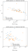Fig. E.1. Relation between p parameter and external field for Milky Way (blue) and Andromeda (orange) satellite dSphs. Uncertainties are not shown to keep the plot legible. The dashed line describes Milgrom's constant, a0. The external field is Newtonian and consists of either the field by the host galaxy E.1a or the internal field of the satellite E.1b. The dependence of p on the host field is more obvious.

Appendix F: Derivation of velocity dispersion independently of density profile

In the following, the velocity dispersion for arbitrary p neglecting the EFE is derived. Furthermore, it is shown that, for arbitrary p, numerical values for the velocity dispersion can only be calculated by specifying a density profile. Milgrom (1994) derived the velocity dispersion for p = 3. This derivation is analogous to his. Milgrom considered the quantity, Q, integrating over phase-space:

$$Q:={\displaystyle \sum _k}\int m_k{f}_k(r,v,t)r·v{\text{d}}^{3}r{\text{d}}^{3}v\hspace{0.5em}.$$(F.1)

m_k are the masses of arbitrary particles (e.g. stars). f_k(r,v,t) is a phase-space-distribution function. Milgrom showed that its time derivative, $\dot{Q}$, can be written as:

$$\dot{Q}=M\langle v^2\rangle (t)-\int \rho (r,t)r·\nabla \mathrm{\Phi }{\text{d}}^{3}r\hspace{0.5em}.$$(F.2)

Here, the finite total mass, M, of the system and the momentary, mass-weighted, 3-D, mean-square velocity, 〈v²〉(t), is introduced. The GPE is used:

$$\nabla ·\left((\mu (x))\nabla \mathrm{\Phi }\right)=4\pi G\rho \hspace{0.5em},$$(F.3)

$$\mu (x):=x^{p-2}\hspace{0.5em},$$(F.4)

$$x:=\frac{\left|\nabla \mathrm{\Phi }\right|}{a_0}\hspace{0.5em}.$$(F.5)

As opposed to Milgrom, μ(x) is here defined in terms of a fixed p>1. Milgrom inserted the density distribution, ρ, described by Eq. (F.3) into Eq. (F.2). Furthermore, F(y) was introduced, such that

$$\mu (x)=\frac{\text{d}F(y)}{\text{d}y},\hspace{0.5em}y=x^2\hspace{0.5em}.$$(F.6)

Since in the case for arbitrary p, μ(x) is defined by Eq. (F.4):

$$F(x^2)=\frac{2}{p}{x}^p\hspace{0.5em}.$$(F.7)

Milgrom showed that $\dot{Q}$ can be written as

$$\dot{Q}=M\langle v^2\rangle (t)+I_1+I_2\hspace{0.5em},$$(F.8)

$$I_1:=-\frac{1}{4\pi G}\int \mu (x)r·\nabla \mathrm{\Phi }\nabla \mathrm{\Phi }·\text{d}s\hspace{0.5em},$$(F.9)

$$I_2:=I_3+I_4\hspace{0.5em},$$(F.10)

$$I_3:=\frac{a_0^2}{8\pi G}\int F(x^2)r·\text{d}s\hspace{0.5em},$$(F.11)

$$I_4:=-\frac{a_0^2}{4\pi G}\int \frac{3}{2}F(x^2)-\mu (x)x^2{\text{d}}^{3}r\hspace{0.5em}.$$(F.12)

Milgrom solved Eq. (F.8) for 〈v²〉(t) and took the long-time average, $\overline{\langle v^2\rangle }$. Doing so for arbitrary p:

$$\overline{\langle v^2\rangle }=-\frac{1}{M}(I_1+I_3+I_4).$$(F.13)

We assume the density distribution to have a sphere with a radius, R, as compact support and ∇Φ at R for arbitrary p to behave like the gravitational acceleration produced by a point mass:

$$\nabla \mathrm{\Phi }=\sqrt[p-1]{\frac{{\mathit{GMa}}_0^{p-2}}{R^2}}{\text{e}}_r\hspace{0.5em}.$$(F.14)

Equation F.9 was evaluated at R:

$$I_1=-\frac{1}{4\pi G}{\left(\frac{\left|\nabla \mathrm{\Phi }\right|}{a_0}\right)}^{p-2}R\left|\nabla \mathrm{\Phi }\right|4\pi R^2\left|\nabla \mathrm{\Phi }\right|$$(F.15)

$$=-\frac{R^3}{G}{a}_0^{2-p}{\left|\nabla \mathrm{\Phi }\right|}^p$$(F.16)

$$=-M\sqrt[p-1]{{\mathit{GMR}}^{p-3}{a}_0^{p-2}}\hspace{0.5em}.$$(F.17)

Equation F.11 was evaluated at R:

$$I_3=\frac{a_0^2}{8\pi G}\frac{2}{p}{\left(\frac{\left|\nabla \mathrm{\Phi }\right|}{a_0}\right)}^{p}4\pi R^3$$(F.18)

$$=\frac{1}{p}\frac{R^3}{G}{a}_0^{2-p}{\left|\nabla \mathrm{\Phi }\right|}^p$$(F.19)

$$=\frac{1}{p}M\sqrt[p-1]{{\mathit{GMR}}^{p-3}{a}_0^{p-2}}\hspace{0.5em}.$$(F.20)

Equation F.12 was evaluated at R:

$$I_4=-\frac{a_0^2}{4\pi G}\int \left(\frac{3}{2}\frac{2}{p}{x}^p-x^{p-2}{x}^2\right){\text{d}}^{3}r$$(F.21)

$$=-\frac{a_0^2}{4\pi G}\int \frac{3-p}{p}{x}^p{\text{d}}^{3}r$$(F.22)

$$=-\frac{a_0^2}{4\pi G}\frac{3-p}{p}{\displaystyle {\int }_0^R}4\pi r^2{\left(\frac{a(r)}{a_0}\right)}^p\text{d}r$$(F.23)

$$=-\frac{a_0^2}{G}\frac{3-p}{p}{\displaystyle {\int }_0^R}{r}^2{\left(\frac{a(r)}{a_0}\right)}^p\text{d}r$$(F.24)

$$=-\frac{1}{G}\frac{3-p}{p}{\displaystyle {\int }_0^R}{r}^2{\left(\frac{a(r)}{a_0}\right)}^{p-2}{a}^2(r)\text{d}r$$(F.25)

$$=-\frac{1}{G}\frac{3-p}{p}{\displaystyle {\int }_0^R}\mathit{GM}(r)a(r)\text{d}r$$(F.26)

$$=\frac{p-3}{p}{\displaystyle {\int }_0^R}M(r)a(r)\text{d}r\hspace{0.5em}.$$(F.27)

I₄ depends on the density distribution. It vanishes only for p = 3 (Milgromian case). This explains why the velocity dispersion is independent of the density distribution only for Milgromian gravity.

All Tables

All Figures

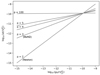	Fig. 1. RAR for arbitrary p. The bold grey lines indicate the RARs for different p (Eq. (5)).
In the text

	Fig. 2. RAR for selected Milky Way (blue) and Andromeda (orange) satellite dSphs and galaxy clusters (green). Uncertainties are 1σ. The data are taken from Lelli et al. (2017) for the dSphs (Milky Way and Andromeda satellites) and Li et al. (2023) for the galaxy clusters, as is tabulated in Tables A.1 and B.1, respectively. The bold grey lines for different p are the same as in Fig. 1.
In the text

	Fig. 3. Relation between density of dSphs (blue and orange) and galaxy clusters (green) and p parameter from GPE, Eq. (1). Uncertainties are 1σ. p was obtained from the RAR, as is shown in Fig. 2. See Tables A.1 and B.1 for values. The red line is an exponential function fit to the data with χ2/ndf = 8.001.
In the text

	Fig. 4. 1D velocity dispersion for selected Milky Way satellite dSphs. Blue are data by Lelli et al. (2017) and orange data by Safarzadeh & Loeb (2021). The black triangles were calculated from the Lelli et al. (2017) data with Eq. (30).
In the text

Fig. 5. Relation between p parameter and external field gtot for Milky Way (blue) and Andromeda (orange) satellite dSphs. The dashed line describes Milgrom's constant a0. Uncertainties are not shown to keep the plot legible (see Tables C.1 and D.1 for uncertainties on p). The external field is Newtonian and consists of the field by the host galaxy and the internal field of the satellite. A logarithmic fit function (solid green curve) described by Eq. (56) suggests a functional relation, p(gtot).

In the text

Fig. E.1. Relation between p parameter and external field for Milky Way (blue) and Andromeda (orange) satellite dSphs. Uncertainties are not shown to keep the plot legible. The dashed line describes Milgrom's constant, a0. The external field is Newtonian and consists of either the field by the host galaxy E.1a or the internal field of the satellite E.1b. The dependence of p on the host field is more obvious.

In the text

References

- Alexander, S. G., Walentosky, M. J., Messinger, J., et al. 2017, ApJ, 835, 233 [Google Scholar]
- Angus, G. W. 2008, MNRAS, 387, 1481 [Google Scholar]
- Binney, J., & Tremaine, S. 2008, Galactic Dynamics: Second Edition (Princeton: Princeton University Press) [Google Scholar]
- Blanchet, L. 2007, Classical Quantum Gravity, 24, 3529 [Google Scholar]
- Brada, R., & Milgrom, M. 2000, ApJ, 541, 556 [NASA ADS] [CrossRef] [Google Scholar]
- Camilli, F., Capitanelli, R., & Vivaldi, M. A. 2017, Nonlinear Anal., 163, 71 [Google Scholar]
- de Boer, T. J. L., Tolstoy, E., Hill, V., et al. 2012, A&A, 544, A73 [NASA ADS] [CrossRef] [EDP Sciences] [Google Scholar]
- Evans, L. C. 1982, J. Differ. Equations, 45, 356 [Google Scholar]
- Heggie, D., & Hut, P. 2003, The Gravitational Million-Body Problem: A Multidisciplinary Approach to Star Cluster Dynamics (Cambridge, UK: Cambridge University Press) [Google Scholar]
- Kroupa, P. 1997, NA, 2, 139 [Google Scholar]
- Kroupa, P. 2008, Initial Conditions for Star Clusters (Netherlands: Springer), 181 [Google Scholar]
- Kroupa, P., Gjergo, E., Asencio, E., et al. 2023, The Many Tensions with Dark-matter Based Models and Implications on the Nature of the Universe [Google Scholar]
- Lelli, F., McGaugh, S. S., Schombert, J. M., & Pawlowski, M. S. 2017, ApJ, 836, 152 [Google Scholar]
- Li, P., Tian, Y., Júlio, M. P., et al. 2023, A&A, 677, A24 [NASA ADS] [CrossRef] [EDP Sciences] [Google Scholar]
- Lindqvist, P. 2015, Notes on the Infinity-Laplace Equation [Google Scholar]
- Lindqvist, P. 2019a, Notes on the Stationary p-Laplace Equation (Cham: Springer) [CrossRef] [Google Scholar]
- Lindqvist, P. 2019b, The Infinity Laplacian (Cham: Springer International Publishing), 69 [Google Scholar]
- Lu, G., & Wang, P. 2008, Commun. Partial Differ. Equations, 33, 1788 [Google Scholar]
- Lüghausen, F., Famaey, B., & Kroupa, P. 2015, CJP, 93, 232 [Google Scholar]
- McGaugh, S., & Milgrom, M. 2013a, ApJ, 766, 22 [NASA ADS] [CrossRef] [Google Scholar]
- McGaugh, S., & Milgrom, M. 2013b, ApJ, 775, 139 [NASA ADS] [CrossRef] [Google Scholar]
- McGaugh, S. S., & Wolf, J. 2010, ApJ, 722, 248 [NASA ADS] [CrossRef] [Google Scholar]
- McGaugh, S. S., Lelli, F., Schombert, J. M., et al. 2021, AJ, 162, 202 [NASA ADS] [CrossRef] [Google Scholar]
- Merritt, D. 2020, A Philosophical Approach to MOND: Assessing theMilgromian Research Program in Cosmology (Cambridge University Press) [CrossRef] [Google Scholar]
- Milgrom, M. 1983, ApJ, 270, 365 [Google Scholar]
- Milgrom, M. 1994, ApJ, 429, 540 [NASA ADS] [CrossRef] [Google Scholar]
- Milgrom, M. 1997, Phys. Rev. E, 56, 1148 [NASA ADS] [CrossRef] [Google Scholar]
- Milgrom, M. 2014, Phys. Rev. D, 89, 024016 [NASA ADS] [CrossRef] [Google Scholar]
- Mistele, T., McGaugh, S., Lelli, F., Schombert, J., & Li, P. 2024, ApJ, 969, L3 [NASA ADS] [CrossRef] [Google Scholar]
- Růžička, M. 2000, Electrorheological Fluids Modeling and Mathematical Theory [Google Scholar]
- Safarzadeh, M., & Loeb, A. 2021, ApJ, 914, L37 [Google Scholar]
- Sánchez-Salcedo, F. J., & Hernandez, X. 2007, ApJ, 667, 878 [CrossRef] [Google Scholar]
- Sanders, R. H. 2021, MNRAS, 507, 803 [NASA ADS] [CrossRef] [Google Scholar]
- Wolf, J., Martinez, G. D., Bullock, J. S., et al. 2010, MNRAS, 406, 1220 [NASA ADS] [Google Scholar]
- Zhang, Y. Y., Andernach, H., Caretta, C. A., et al. 2011, A&A, 526, A105 [NASA ADS] [CrossRef] [EDP Sciences] [Google Scholar]