| Issue |
A&A
Volume 698, June 2025
|
|
|---|---|---|
| Article Number | A137 | |
| Number of page(s) | 17 | |
| Section | Stellar atmospheres | |
| DOI | https://doi.org/10.1051/0004-6361/202554510 | |
| Published online | 09 June 2025 | |
Discovery of λ Boo stars in open clusters
1
Instituto de Ciencias Astronómicas, de la Tierra y del Espacio (ICATE-CONICET),
C.C 467,
5400
San Juan,
Argentina
2
Universidad Nacional de San Juan (UNSJ), Facultad de Ciencias Exactas, Físicas y Naturales (FCEFN),
San Juan,
Argentina
3
Departamento Astronomía, Universidad de La Serena,
av. Raúl Bitrán 1305,
La Serena,
Chile
4
Observatorio Astronómico de Córdoba (OAC),
Laprida 854,
X5000BGR
Córdoba,
Argentina
5
Consejo Nacional de Investigaciones Científıcas y Técnicas (CONICET),
Argentina
★ Corresponding author.
Received:
13
March
2025
Accepted:
10
April
2025
Abstract
Context. The origin of λ Boo stars is currently unknown. After several efforts by many authors, no bona fide λ Boo stars have been confirmed as members of open clusters. Their detection could provide an important test bed for a detailed study of λ Boo stars.
Aims. Our aim is to detect, for the first time, λ Boo stars as members of open clusters. The λ Boo class will be confirmed through a detailed abundance analysis, while the cluster membership will be evaluated using a multi-criteria analysis of probable members.
Methods. We cross-matched a homogeneous list of λ Boo stars with a Gaia DR3 catalog of open clusters and, notably, we found two candidate λ Boo stars in open clusters. We carried out a detailed abundance determination of the candidate λ Boo stars and additional cluster members via spectral synthesis. Stellar parameters were estimated by fitting observed spectral energy distributions (SEDs) with a grid of model atmospheres using the online tool VOSA, Gaia DR3 parallaxes, and the PARAM 1.3 interface. Then, the abundances were determined iteratively for 22 different species by fitting synthetic spectra using the SYNTHE program together with local thermodynamic equilibrium (LTE) ATLAS12 model atmospheres. The abundances of the light elements C and O were corrected by non-LTE effects. The complete chemical patterns of the stars were then compared to those of λ Boo stars. We also performed an independent cluster membership study using Gaia photometry and radial velocities with a multi-criteria analysis.
Results. For the first time, we present the surprising finding of two λ Boo stars as members of open clusters: HD 28548 belongs to the cluster HSC 1640 and HD 36726 belongs to the cluster Theia 139. This was confirmed using a detailed abundance analysis, while the cluster membership was independently analyzed using Gaia DR3 data and radial velocities. We compared the λ Boo star HD 36726 with other cluster members and showed that the λ Boo star was originally born with a near-solar composition. This also implies one of the highest chemical differences detected between two cluster members (~0.5 dex). In addition, we suggest that the λ Boo peculiarity strongly depletes heavier metals, but could also slightly modify lighter abundances such as C and O. We also found that both λ Boo stars belong to the periphery of their respective clusters. This would suggest that λ Boo stars avoid the strong photoevaporation by UV radiation from massive stars in the central regions of the cluster. We preliminarily suggest that peripheral location appears to be a necessary, though not sufficient, condition for the development of λ Boo peculiarity. We also obtained a precise age determination for the λ Boo stars HD 28548 (26.3±1.4 Myr) and HD 36726 (33.1±1.1 Myr), which are among the most precise age determinations of λ Boo stars. We strongly encourage analyzing additional cluster members, which could provide important insights for the study of the origin of λ Boo stars.
Conclusions. We have confirmed, for the first time, that two λ Boo stars belong to open clusters. This remarkable finding could make open clusters excellent laboratories for studying the origin of λ Boo stars.
Key words: stars: abundances / stars: atmospheres / stars: chemically peculiar
© The Authors 2025
 Open Access article, published by EDP Sciences, under the terms of the Creative Commons Attribution License (https://creativecommons.org/licenses/by/4.0), which permits unrestricted use, distribution, and reproduction in any medium, provided the original work is properly cited.
This article is published in open access under the Subscribe to Open model. This email address is being protected from spambots. You need JavaScript enabled to view it. to support open access publication.
1 Introduction
For many years, the nature of the λ Boo stars has been controversial. They are a class of metal-poor Population I A-type stars first discovered in the work of Morgan et al. (1943). The λ Boo stars are markedly metal deficient (up to ~2 dex in the most extreme cases), but have nearly solar abundances of the lighter elements CNO and S (e.g. Kamp et al. 2001; Andrievsky et al. 2002; Heiter et al. 2002; Alacoria et al. 2022). Most λ Boo stars are discovered through spectral classification (see, e.g., Murphy et al. 2015; Gray et al. 2017; Murphy et al. 2020), although a detailed abundance determination has been suggested to confirm their membership in the class (e.g., Andrievsky et al. 2002; Heiter et al. 2002; Murphy et al. 2015; Gray et al. 2017; Alacoria et al. 2022, 2025). These rare stars (about ~2% of the A-type stars, Gray & Corbally 1998; Paunzen 2001) present a considerable challenge to our understanding of stellar atmospheres.
The detection of λ Boo stars as members of multiple systems is important for several reasons. For instance, this could help to precisely determine their evolutionary state, which motivated searches of λ Boo stars in open clusters by several authors (e.g., Paunzen & Gray 1997; Gray & Corbally 1998; Paunzen et al. 2001; Paunzen 2001; Gray & Corbally 2002; Paunzen et al. 2003b, 2014). Furthermore, the composition of late-type stars in a multiple system could be used as a proxy of the initial composition from which λ Boo stars were born (e.g., Alacoria et al. 2022, 2025). In addition, the comparison of a λ Boo star with other early-type stars in the system could be used to test formation models such as the interaction with a diffuse cloud (see, e.g., Paunzen et al. 2012a,b; Alacoria et al. 2022). The works mentioned assume that multiple systems are a single population of co-evolutionary stars, meaning that the stars formed together from the same molecular cloud. In this way, the detection of λ Boo stars in multiple systems is considered a valuable discovery, and provides a key laboratory to study their origin in detail.
However, detecting λ Boo stars as members of multiple systems has proven to be a difficult task. For the case of binary systems, Paunzen et al. (2012a,b) identified about a dozen λ Boo stars as members of early-type binary systems, while Alacoria et al. (2025) recently identified new systems including late-type companions. On the other hand, to our knowledge no bona fide λ Boo star is known as a member of an open cluster. In order to determine the evolutionary state of λ Boo stars, extensive searches were performed in 32 different open clusters (see, e.g., Paunzen & Gray 1997; Gray & Corbally 1998; Paunzen et al. 2001; Paunzen 2001; Gray & Corbally 2002; Paunzen et al. 2003b, 2014). The searches mentioned mainly included intermediate-age open clusters, that is, with ages between 107 yr and 109 yr, approximately. Notably, although several chemically peculiar Am and Ap stars were detected in the same clusters (e.g., Gray & Corbally 2002; Paunzen et al. 2014), no λ Boo stars were identified. For instance, Paunzen & Gray (1997) and Paunzen et al. (2001) reported a candidate λ Boo star in the open cluster NGC 2264 (HD 261904 = NGC 2264 # 138) and three candidates in the periphery of the Orion OB1 association. However, Andrievsky et al. (2002) determined suprasolar abundances for Mg and Fe in HD 261904, while Murphy et al. (2015) classified this object as an uncertain member of the λ Boo class. We also note that the Orion OB1 association presents subgroups of stars (OB1a, OB1b, OB1c, and OB1d) with different ages and dynamical properties, rather than a single population (see, e.g., Bally 2008, and references therein). The examples mentioned illustrate that the detection of λ Boo stars in multiple systems is a challenging task and deserves to be explored further.
With the aim of providing a consistent and homogeneous membership of λ Boo stars, a number of works reevaluated every λ Boo star previously reported in the literature (see Murphy et al. 2015; Gray et al. 2017; Murphy et al. 2020). Together, these three works comprise a complete and homogeneous sample of 118 (predominantly southern) λ Boo stars. On the other hand, Hunt & Reffert (2024) performed a blind all-sky search for open clusters using Gaia DR3 data of 729 million stars down to magnitude G~20, and recovered 5647 bound open clusters (1441 of which are new detections). Then, with the aim of detecting λ Boo stars in multiple systems, we cross-matched the list of 118 λ Boo stars with this catalog of clusters. Surprisingly, we found two λ Boo stars with a very high membership probability: HD 28548 member of HSC 1640 (Prob~95%, log t~7.2) and HD 36726 member of Theia 139 (Prob~100%, log t~8.0). In particular, HD 36726 is one of the three λ Boo stars reported by Paunzen & Gray (1997) as a member of the Orion OB1 association. We note that HSC 1640 and Theia 139 are classified as open clusters in different works (Hunt & Reffert 2023; Cavallo et al. 2024), while Hunt & Reffert (2024) caution that both clusters are possibly dissolving; we return to this point in the discussion. The remarkable finding of these two λ Boo stars encourages us to study them as well as other members of their multiple systems. This could provide the possibility of having a valuable test bed for a detailed study of λ Boo stars.
In this work, we present a detailed chemical analysis of two candidate λ Boo stars together with other objects that belong to the same multiple system. This would first require confirming the λ Boo class of the two candidates with a detailed chemical analysis, and then verifying that the stars in the multiple system belong to a single population through a membership analysis. We analyzed the chemical composition of both stars together with additional cluster members, with an initial membership suggested by the work of Hunt & Reffert (2024). We also performed an independent membership study using a multi-criteria analysis, showing that both candidate λ Boo stars are members of their multiple systems. However, some of the additional stars analyzed should be taken with caution. Studying λ Boo stars along with their stellar siblings1 could provide important insights into the origin of λ Boo stars.
This work is organized as follows. In Sect. 2, we describe the sample and observations. In Sect. 3, we present the stellar parameters and chemical abundance analysis. In Sect. 4, we present our independent cluster membership analysis, and in Sect. 5, we discuss the results. Finally, in Sect. 6 we highlight our main conclusions.
2 Sample and observations
The sample of stars used in this work was derived as follows. The candidate λ Boo stars HD 28548 and HD 36726 were obtained by cross-matching the homogeneous list of 118 λ Boo stars with the cluster catalog of Hunt & Reffert (2024), as previously explained. Then, additional cluster members were initially suggested by selecting relatively bright stars with high membership probability (>90%) in the same cluster catalog (Hunt & Reffert 2024). We derived a detailed chemical composition for all these stars. Then, we performed an independent membership analysis including radial velocities and confirmed that both candidate λ Boo stars are members of the clusters, while some of the additional stars do not appear to be true cluster members. Our cluster membership analysis including an age derivation for the clusters, is presented in Section 4.
We present in Table 1 the visual magnitude V, coordinates, proper motions, parallax, and signal-to-noise per pixel (at 5500 Å) for the stars studied in this work. The spectral data for the stars in this work were acquired through the Gemini High-resolution Optical SpecTrograph (GHOST), which is attached to the 8.1 m Gemini South telescope at Cerro Pachón, Chile. GHOST is illuminated via 1.2″ integral field units that provide the input light apertures. The spectral coverage of GHOST in the range 360–900 nm is appropriate for deriving stellar parameters and chemical abundances using several features. It provides a high resolving power R~50 000 in the standard resolution mode2. The read mode was set to medium, as recommended for relatively bright targets. The observations were taken between October 4, 2024, and October 26, 2024 (PI: Carlos Saffe, Program ID: GS-2024B-FT-210), under a fast turnaround (FT) observing mode3, using the same spectrograph configuration for all stars. The exposure times varied between 40 sec and 280 sec, depending on the star; an average signal-to-noise ratio (S/N) of ~315 per pixel measured near ~5500 Å was obtained. The spectra were reduced using the GHOST data reduction pipeline v1.1.0, which works under DRAGONS4. This is a platform for the reduction and processing of astronomical data.
Magnitudes and astrometric data for the stars analyzed in this work.
 |
Fig. 1 Spectral energy distribution (black circles) and synthetic spectra (blue continuous line) corresponding to the stars HD 28548 and HD 36726 (left and right panels). |
3 Stellar parameters and abundance analysis
We estimated the effective temperatures (Teff) for the stars in our sample by using the Virtual Observatory SED Analyzer5 (VOSA, Bayo et al. 2008). This tool allows the fitting of spectral energy distributions (SEDs) constructed from photometric data using different atmospheric models. Observed SEDs were unreddened by VOSA using the extinction maps of Schlegel et al. (1998) and following the procedure of Bilir et al. (2008) to derive Av. We used a grid of Kurucz-NEWODF models (Kurucz 1993) covering Teff between 3500–13 000 K, with steps of 250 K. We present an example of the observed and synthetic SEDs for the stars HD 28548 and HD 36726 in Fig. 1. Then, we performed a Bayesian estimation of surface gravities log g using Gaia DR3 parallaxes with the PARAM 1.3 interface6 (da Silva et al. 2006). The temperatures and gravities derived for the stars in our sample are presented in Table 2.
In the next step, we estimated the projected rotational velocities v sin i by fitting the line Mg II 4481.23 Å and then refined the selection by fitting most Fe I and Fe II lines in the spectra, similarly to previous works (Saffe & Levato 2014; Saffe et al. 2020, 2021). Synthetic spectra were calculated using the program SYNTHE (Kurucz & Avrett 1981) together with ATLAS12 (Kurucz 1993) model atmospheres. These spectra were then convolved with a rotational profile and with an instrumental profile for the GHOST spectrograph (resolving power R ~ 50 000). The resulting v sin i values are shown in Col. 6 of Table 2, covering between 22.4 ± 1.6 km s−1 and 129.6 ± 2.7 km s−1 for the stars in our sample. The microturbulence velocity (vmicro) was estimated as a function of Teff following the formula of Gebran et al. (2014), which is valid for ~6000 K < Teff < ~10 000 K. We adopted an uncertainty of ~25% for vmicro, as suggested by Gebran et al. (2014), and then this uncertainty was taken into account in the abundance error calculation.
Chemical abundances were determined by applying an iterative procedure, similar to previous works (e.g., Saffe et al. 2020, 2021, 2022; Alacoria et al. 2022, 2025). We started the process by initially adopting solar abundances from Asplund et al. (2009) and deriving an ATLAS12 (Kurucz 1993) model atmosphere. The corresponding abundances were then obtained by fitting the observed spectra with the program SYNTHE (Kurucz & Avrett 1981). With the new abundance values, we derived a new model atmosphere and restarted the process again. In each step, the opacities were calculated for an arbitrary composition and vmicro using the opacity sampling (OS) method. In this way, the parameters and abundances were consistently derived using specific opacities rather than solar-scaled values, until the same input and output abundance values were reached (for more details, see Saffe et al. 2021). Possible differences originating from the use of solar-scaled opacities instead of an arbitrary composition were recently estimated for the case of solar-type stars (Saffe et al. 2018, 2019).
We derived the chemical abundances for 22 different species, including Li I, C I, O I, Na I, Mg I, Mg II, Al I, Si II, Ca I, Ca II, Sc II, Ti II, Cr II, Mn I, Fe I, Fe II, Co I, Ni II, Zn I, Sr II, Y II, and Ba II. The atomic line list and laboratory data used in this work are the same as described in previous works from our team (Saffe et al. 2021, 2022; Alacoria et al. 2022, 2025). Figure 2 presents an example of the observed, synthetic, and difference spectra (black, blue dotted, and magenta lines) for some stars in our sample. There is a good agreement between modeling results and observations for the lines of different chemical species.
For each individual species, we estimated the uncertainty in the corresponding abundance value by including different sources. The measurement error, e1, was estimated from the line-to-line dispersion as ![Mathematical equation: $\[\sigma / \sqrt{n}\]$](/articles/aa/full_html/2025/06/aa54510-25/aa54510-25-eq1.png) , where σ is the standard deviation and n is the number of lines. For elements with only one line, we adopted for σ the standard deviation of the iron lines. Then, we determined the contribution to the abundance error due to the uncertainty in stellar parameters. We modified Teff, log g, and vmicro by their uncertainties and recalculated the abundances, obtaining the corresponding differences e2, e3, and e4; we adopted a minimum of 0.01 dex for these errors. Finally, the total error etot was estimated as the quadratic sum of e1, e2, e3, and e4. We discuss the chemical pattern for each star in Appendix A, comparing them with an average pattern of λ Boo stars and other chemically peculiar stars. The average pattern of λ Boo stars is the same as used in Alacoria et al. (2022); basically, we adopted the data derived by Heiter et al. (2002), but excluded those stars without CNO values. The abundances with their total error etot, the individual errors e1 to e4, and the number of lines n are presented in Tables B.1 to B.10 of Appendix B.
, where σ is the standard deviation and n is the number of lines. For elements with only one line, we adopted for σ the standard deviation of the iron lines. Then, we determined the contribution to the abundance error due to the uncertainty in stellar parameters. We modified Teff, log g, and vmicro by their uncertainties and recalculated the abundances, obtaining the corresponding differences e2, e3, and e4; we adopted a minimum of 0.01 dex for these errors. Finally, the total error etot was estimated as the quadratic sum of e1, e2, e3, and e4. We discuss the chemical pattern for each star in Appendix A, comparing them with an average pattern of λ Boo stars and other chemically peculiar stars. The average pattern of λ Boo stars is the same as used in Alacoria et al. (2022); basically, we adopted the data derived by Heiter et al. (2002), but excluded those stars without CNO values. The abundances with their total error etot, the individual errors e1 to e4, and the number of lines n are presented in Tables B.1 to B.10 of Appendix B.
Fundamental parameters derived for the stars in this work.
 |
Fig. 2 Observed, synthetic, and difference spectra (black, blue dotted, and magenta lines) for some stars in our sample. |
3.1 NLTE effects
In the upper main sequence, a parameter space occupied by λ Boo stars, non-local thermodynamic equilibrium (NLTE) abundance corrections are relevant for light-elements (see, e.g., Paunzen et al. 1999; Alacoria et al. 2022, 2025). For instance, an average O I correction of −0.5 dex was derived by Paunzen et al. (1999) for a sample of λ Boo stars; instead, for C I they estimated an average correction of −0.1 dex. Rentzsch-Holm (1996) derived neutral carbon NLTE abundance corrections by using a multi-level model atom for stars with Teff between 7000 K and 12 000 K, log getween 3.5 and 4.5 dex, and metallicity between −0.5 dex and +1.0 dex. She showed that C I NLTE effects are negative (calculated as NLTE-LTE) and depend primarily on equivalent width Weq. Near ~7000 K, the three lower levels of C I are always in LTE; however, increasing the Teff values increases the underpopulation of these levels respect to LTE by UV photoionization. Thus, we estimated NLTE abundance corrections of C I for the stars in our sample by interpolating in their Figs. 7 and 8 as a function of Teff, Weq, and metallicity. We applied a similar correction in previous works (Alacoria et al. 2022, 2025), which allows the comparison of abundance values.
For the case of O I, we performed NLTE abundance corrections following the work of Sitnova et al. (2013), who determined LTE and NLTE abundances using a model atom with 51 levels. Sitnova et al. (2013) showed that NLTE effects lead to a strengthening of O I lines, producing a negative NLTE correction. They calculated NLTE corrections for a grid of model atmospheres, including stars with spectral types from A to K (Teff between 10 000 and 5000 K). Then, we estimated NLTE abundance corrections of O I (IR triplet 7771 Å) for the stars in this work, interpolating based on Table 11 of Sitnova et al. (2013), as a function of Teff. We note that other O I lines present corrections lower than ~−0.02 dex (see, e.g., Table 5 of Sitnova et al. 2013).
4 Membership in open clusters
For this section we analyzed the membership of all the stars in our sample in the open clusters HSC 1640 and Theia 139, including the λ Boo stars HD 28548 and HD 36726. We applied a multi-criteria analysis to determine the cluster membership using a kinematic and photometric selection of probable members, following a procedure similar to previous works (e.g., Alejo et al. 2020). We used the initial membership suggested by Hunt & Reffert (2024) for each cluster (using astrometric and photometric Gaia DR3 data, Gaia Collaboration 2023), but also complemented with the radial velocities available in the literature and measured in our spectra (see Table C.1 of Appendix C).
First, we determined a kinematic membership by comparing individual radial velocities with the cluster mean, adopting a criterion based on their uncertainty. We measured the radial velocities of all observed stars by cross-correlation using the IRAF task fxcor with the GHOST spectra. In the selection of spectral regions, we excluded hydrogen lines, interstellar lines, and regions lacking spectral lines. The template spectra for the cross-correlations were selected from the database of Bertone et al. (2008). The synthetic templates were then convolved with appropriate rotational profiles. The relative velocities between objects and templates were measured by fitting a Gaussian to the correlation peak. We also took into account the radial velocities obtained from the surveys RAVE DR6 (Steinmetz et al. 2020), Gaia DR3 (Gaia Collaboration 2023), and APOGEE (Jönsson et al. 2020). Gaia DR3 velocities were corrected, as proposed by Katz et al. (2023), for those stars where the integrated Grvs magnitude is Grvs ≥ 11 mag, and for stars where 6 mag ≤ Grvs ≤ 12 mag, according to Blomme et al. (2023). Because we have few spectra and few radial velocity measurements, we do not rule out that some objects may present spectroscopic variability. For those stars with more than one radial velocity measurement, we calculated the average velocity (![Mathematical equation: $\[\bar{V}\]$](/articles/aa/full_html/2025/06/aa54510-25/aa54510-25-eq2.png) ) and its uncertainty (
) and its uncertainty (![Mathematical equation: $\[\varepsilon_{\bar{V}}\]$](/articles/aa/full_html/2025/06/aa54510-25/aa54510-25-eq3.png) ) using the expressions of González & Lapasset (2000). In those equations, the error is calculated considering both the individual errors and the dispersion of the measurements. The results of these calculations are listed in Table C.1. In particular, we note that the star HD 290572 in Theia 139 is a spectroscopic binary (Gaia Collaboration 2022), so we used its center-of-mass velocity in the calculations.
) using the expressions of González & Lapasset (2000). In those equations, the error is calculated considering both the individual errors and the dispersion of the measurements. The results of these calculations are listed in Table C.1. In particular, we note that the star HD 290572 in Theia 139 is a spectroscopic binary (Gaia Collaboration 2022), so we used its center-of-mass velocity in the calculations.
To calculate the cluster mean radial velocity and determine the kinematic membership, we analyzed the radial velocity distribution of the observed stars, those available in the bibliography and probable members according to Hunt & Reffert (2024). First, we fitted the radial velocity distribution with the Leven-berg–Marquardt least-squares optimization technique from the SciPy library in PYTHON, and obtained a first mean value for each cluster. We used a bin size of 1 km s−1 in the calculation. Taking into account this mean cluster velocity, the radial velocity of the stars, and their uncertainties, we adopted a selection criterion based on uncertainty. We selected as probable radial velocity members those stars whose radial velocity difference with the cluster mean is smaller than its uncertainty, a criterion previously adopted by Alejo et al. (2020). In the final calculation of the radial velocity of the cluster we included all stars classified as members. Since radial velocity uncertainty could vary from star to star, in the cluster mean we applied weights proportional to (ϵ2 + Δ2)−1, where ϵ is the uncertainty of the star radial velocity and Δ = 1 km s−1. The reason for including the constant Δ is that the radial velocity of an individual star, as an estimator of the mean cluster velocity, has an uncertainty of at least the internal velocity of the cluster, which in open clusters is typically on the order of 1 km s−1. The final values of the mean radial velocity of the clusters are 13.2 ± 0.4 km s−1 for HSC 1640 and 16.3 ± 0.3 km s−1 for Theia 139. In this way, we found that the λ Boo stars HD 28548 and HD 36726 are probable radial velocity members (see Table 3).
Then, we performed a photometric selection of probable members, taking into account their position in the color–magnitude diagram. We made this selection and also obtained the age of the clusters using an iterative PYTHON script. Briefly, we started the iterations by providing an approximate value of extinction and cluster age. The algorithm determines the parallax and average metallicity weighted with Gaia data. With this information, the script selects an isochrone (then used to fit the photometric data) and derives new values for the parallax and extinction. We used a grid of PARSEC stellar models (Bressan et al. 2012; Nguyen et al. 2022) with isochrones between log τ = 6.00 and log τ = 8.85 and metallicity between [Fe/H]=−0.3 dex and [Fe/H]=+0.3 dex. Next, the algorithm uses the bootstrap technique to randomly select and replace a number of stars (equal to the number of probable cluster members). In every fit, the script determines the residuals weighted by the error in magnitude and color, and selects the fit with the minimum residual. Then, the program considers the location of the stars in the color–magnitude diagram to detect non-members of the cluster. In this case, the script determines the minimum distance of the stars to the isochrone (d) and rules out those objects with a d >0.7 mag. The final isochrone corresponds to the one with the minimum residuals. Figures 3 and 4 show the G versus (GBP − GRP) color–magnitude diagram of probable members of the two clusters and the isochrone fit corresponding to log τ =7.42±0.14 for HSC 1640 and 7.52±0.05 for Theia 139. Finally, the program performs a new determination of parallax and extinction.
Once we had made the kinematic and photometric selection of probable members, we calculated the cluster parameters by averaging all stars weighted with the membership probability and its uncertainty. In Table 4, we list the spectroscopic, astrometric, and photometric parameters obtained for both clusters. Considering the observed objects, we found that HD 28548 is a probable member of the cluster HSC 1640, while the stars HD 36726, HD 37187, and HD 290621 are probable members of the cluster Theia 139. In Figures 3 and 4, we show the distribution of probable members (gray circles) in different spaces, including the color–magnitude diagram (upper left), position (upper right), proper motion (lower left), and parallax space (lower right). The position of the λ Boo stars is indicated in the plots (blue diamonds). The cluster center is also marked in the coordinate space (red plus signs). The best isochrone found by the script is shown with a continuous red line in the color – magnitude diagram (upper left panel of Figs. 3 and 4). We can see from Figs. 3 and 4 that the λ Boo stars are located on the periphery of the clusters.
Average radial velocities and membership for the stars in our sample.
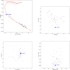 |
Fig. 3 Distribution of probable members of the cluster HSC 1640 (gray circles) in different spaces, including the color–magnitude diagram (upper left), position (upper right), proper motion (lower left), and parallax space (lower right). The position of the λ Boo stars is indicated in the plots (blue diamonds). The cluster center is marked in the coordinate space (red plus signs). The best isochrone fit is shown with a red continuous line in the color–magnitude diagram (upper left). |
5 Discussion
5.1 The nature of HSC 1640 and Theia 139
HSC 1640 is considered an open cluster in several works (Hunt & Reffert 2023; Cavallo et al. 2024; Hu et al. 2024; Maconi et al. 2025). Theia 139 is also considered an open cluster in different works (Hunt & Reffert 2023; Cavallo et al. 2024; Faltová et al. 2025). Both clusters are included in The Unified Cluster Catalog (UCC7). However, Hunt & Reffert (2024) caution that both clusters are possibly dissolving. They attempted to separate bound and unbound clusters, and identified them as open clusters (OCs) and moving groups (MGs). First, they applied a membership algorithm with the main aim of identifying open clusters, that is, a single population, and then they classified the clusters found in MGs and OCs. The separation was performed by estimating the probability that a given cluster has a valid Jacobi radius. Then, the authors consider that those clusters classified as MGs are dissolving into the disk. In this way, they classified HSC 1640 and Theia 139 as OCs in a first work (Hunt & Reffert 2023) and then as MGs when applying the Jacobi radius criterion in a subsequent work (Hunt & Reffert 2024). However, they caution that the Jacobi radius method could present serious limitations in the case of low mass clusters (such as HSC 1640 and Theia 139). For these low mass clusters, they caution that the Jacobi radii may be erroneously calculated and even show some examples. Therefore, we consider that the classification of HSC 1640 and Theia 139 as MGs should be taken with caution.
We also note the following. In general, MGs are usually defined as stars with similar spatial and kinematic properties (e.g., Antoja et al. 2008, 2010). The origin of MGs is attributed to different mechanisms, such as the trapping of stars by Galactic resonances and/or the dissolution of open clusters (e.g., Antoja et al. 2010; Barros et al. 2020; Gagné et al. 2021; Yang et al. 2021). A number of MGs display a very wide range of ages (e.g., Antoja et al. 2008; Kushniruk et al. 2020), implying a mix of stellar populations. For example, the moving group HR 1614 presents a wide range of ages and metallicity (Kushniruk et al. 2020), while Yang et al. (2021) discussed some examples of MGs which include a mixture of thin and thick disk stars. The examples mentioned show that, in general, MGs do not represent a single population of stars. However, this differs from the criterion adopted by Hunt & Reffert (2024) to separate MGs and OCs; in their work, both MGs and OCs are considered a single population, separated only by the Jacobi radius criterion. We suppose that Hunt & Reffert (2024) intended to separate bound from unbound objects, rather than provide a precise definition of MGs. Taking into account the mentioned limitations of the Jacobi radius criterion, we consider it appropriate to refer to HSC 1640 and Theia 139 as possibly dissolving open clusters. Beyond the classification of HSC 1640 and Theia 139 (OCs, MGs, or multiple systems), the most relevant aspect for the study of λ Boo stars is that the two groups belong to a single population, as shown by Hunt & Reffert (2023); Hunt & Reffert (2024) and also verified in this work with a multi-criteria analysis (Section 4).
 |
Fig. 4 Distribution of probable members of the cluster Theia 139 (gray circles) in different spaces, including the color–magnitude diagram (upper left), position (upper right), proper motion (lower left), and parallax space (lower right). The position of the λ Boo stars is indicated in the plots (blue diamonds). The cluster center is marked in the coordinates space (red plus signs). The best isochrone fit is shown with a red continuous line in the color–magnitude diagram (upper left). |
Parameters of the clusters HSC 1640 and Theia 139.
5.2 λ Boo stars in the cluster Theia 139
Following our membership analysis (Section 4 and Table C.1), we found three stars that belong to the cluster Theia 139: HD 36726, HD 37187, and HD 290621. However, the other two stars analyzed (HD 37333 and HD 290541) do not seem to belong to the same population. In addition, our abundance analysis showed that HD 36726 exhibits a λ Boo chemical pattern. Then, this remarkable finding implies that the λ Boo star HD 36726 could be analyzed together with other stellar siblings (e.g., HD 37187 and HD 290621), in order to study the origin of λ Boo stars. We note that HD 36726 is one of the three λ Boo stars reported by Paunzen & Gray (1997) as members of the Orion OB1 association. On this occasion, we confirmed its λ Boo class and verified its membership in a stellar population.
To estimate the original chemical composition of Theia 139, it is reasonable to consider the two non-peculiar stars in our sample, namely HD 37187 and HD 290621. Both stars display mostly solar or slightly subsolar composition, and their metallicities agree well within the errors ([FeI/H]=−0.09±0.15 dex and [FeI/H]=−0.12±0.18 dex). The agreement between the two stars supports the idea that they belong to the same population. However, HD 37187 is significantly hotter than HD 290621 (their Teff are 10500±250 K and 7000±250 K). Considering that diffusion effects are more pronounced in early-type stars compared to late-type objects (see, e.g., Dotter et al. 2017), HD 290621 should present, in principle, a chemical composition closer to that of the original cloud of Theia 139.
In order to determine the magnitude of the λ Boo phenomenon, we can compare the λ Boo star HD 36726 with a proxy for the original composition of Theia 139, that is, HD 290621. There is a significant difference in the composition of the two stars, as we can see in Figs. A.6 and A.9. These two stars present one of the greatest differences found between two siblings that belong to the same population. For instance, their metallicities differ by ~0.5 dex ([FeI/H]=−0.72±0.2 dex and [FeI/H]=−0.12±0.18 dex). This strengthens the idea that λ Boo stars were born with a near-solar composition, which is similar to a recent result (Alacoria et al. 2022, 2025). It is also interesting to note that the lithium is intense in HD 290621 ([Li/H]=2.07±0.21 dex), whereas it is not detected in the λ Boo star HD 36726. A similar observation about Li was noted by Alacoria et al. (2025), who found Li in some stars, but not in their λ Boo binary companions. We caution that the Li abundance is sensitive to different factors, such as age, metallicity (e.g., Martos et al. 2023), and even planet engulfment events (e.g., Saffe et al. 2017; Flores et al. 2024; Miquelarena et al. 2024), which are not necessarily related to the λ Boo phenomenon. Regarding the abundances of other light elements, C resulted lower in the λ Boo star HD 36726 compared to HD 290621 ([C/H]=−0.80±0.18 dex and [C/H]=−0.13±0.18 dex); however, O resulted similar in both stars ([O/H]=−0.29±0.12 dex and [O/H]=−0.21±0.11 dex). Thus, the λ Boo phenomenon produces a significant variation in the heavier elements and, perhaps, a less significant but still noticeable variation in the lighter elements, in agreement with the result of Alacoria et al. (2025). We caution that the C and O abundances were corrected by NLTE effects. Therefore, we cannot completely discard that NLTE effects possibly played a role in this comparison. It would be valuable to confirm this result for the case of the cluster HSC 1640.
A number of works have explored the possibility that IR excesses could be related to λ Boo stars. However, there is no conclusive evidence supporting this relationship (e.g., Paunzen et al. 2003a; Draper et al. 2016; Gray et al. 2017; Murphy et al. 2020). We present in Fig. 1 (right panel) an example of the observed and modeled SEDs of the star HD 36726. Interestingly, we find an IR excess at the WISE band W4; however, no clear excess is present in HD 37187 or in HD 290621. Nevertheless, we caution that a larger sample of stars would help shed light on this possible relationship.
It would be interesting to determine why the λ Boo phenomenon only developed in HD 36726 but not in HD 37187 or HD 290621. We show in Section 4 that the three stars belong to the same stellar population (Theia 139). We started by exploring the Teff of these stars. For HD 36726, HD 37187, and HD 290621 we obtained Teff values of 9000±250 K, 10500±250 K, and 7000±250 K. These temperatures would approximately correspond to spectral types A2, B9, and F1 (adopting the temperature scale of Kenyon & Hartmann 1995, their Table 5). The homogeneous list of 118 λ Boo stars present (hydrogen) spectral types ranging between B8/B9 and F5 (Murphy et al. 2015; Gray et al. 2017; Murphy et al. 2020). Therefore, we cannot disregard that the Teff possibly played a role in helping to avoid the development of the λ Boo phenomenon, especially for the hot star HD 37187. However, the presence of 22 F1-type objects in the list of 118 λ Boo stars, suggests that the λ Boo phenomenon could still operate at the Teff of HD 290621. This would imply that other factor beyond the Teff possibly avoided the λ Boo phenomenon in HD 290621. The rotational velocities vsini of HD 36726 and HD 290621 are not very different (99.6 ± 0.9 km/s and 106.4 ± 1.4 km/s). Perhaps the lack of an IR excess (i.e., the absence of a circumstellar disk) around HD 290621 played a role. However, the relationship between IR excess and λ Boo stars should be taken with caution, as previously explained.
We note that the λ Boo star HD 36726 belongs to the periphery of Theia 139 rather than to the central regions (see Fig. 4). Gray & Corbally (2002) discussed the lack of λ Boo stars in open clusters and mentioned that few candidate λ Boo stars are found in the periphery of star-forming regions (the Orion Nebula). They suggested that this is due to the presence of a factor external to the star and related to membership in open clusters that prevents the λ Boo mechanism. They later concluded that, possibly, the factor is the photoevaporation by UV radiation from massive O-type cluster stars of the circumstellar disk material (which otherwise would be accreted producing the λ Boo phenomenon). In this way, they suggested that the present field λ Boo stars would have formed essentially in isolation or on the peripheries of these star-forming regions. Gray & Corbally (2002) also noted that this would be in agreement with the accretion scenario of Venn & Lambert (1990), a theory for the λ Boo mechanism that requires the accretion of metal-depleted gas from interstellar or circumstellar material. Simulations also show that circumstellar disks close to the cluster density centers are more strongly affected by external photoevaporation than those further out (see, e.g., Fig. 2 of Huang et al. 2024). However, we caution that the effect of external photoevaporation on circumstellar disks depends on several factors (see, e.g., the recent review of Winter & Haworth 2022, and references therein). For example, Adams et al. (2006) suggested that the effect of photoevaporation is relatively small in small clusters with 100–1000 members (as in the case of Theia 139). Then, although the photoevaporation scenario is encouraging (explaining the lack of λ Boo stars in clusters), we consider that it should be taken with caution. Gray & Corbally (2002) claim that no other λ Boo scenario seems able to account for the lack of λ Boo in open clusters and the presence of λ Boo stars in the peripheries.
The location of early-type stars in the periphery of clusters does not seem to be the only requirement for the development of λ Boo stars. We analyzed three members of Theia 139: the λ Boo star HD 36726, as well as HD 37187 and HD 290621. The stars HD 36726 and HD 290621 are both located in the periphery of Theia 139, while HD 37187 is closer to the center. However, the λ Boo phenomenon only developed in HD 36726, but not in HD 290621 (and the Teff of HD 290621 does not seem to preclude the λ Boo phenomenon). This would preliminarily suggest that peripheral location appears to be a necessary, though not sufficient, condition for the development of the λ Boo peculiarity. We have already noted that there is an IR excess in HD 36726, but not in HD 290621. Perhaps, only HD 36726 presents a circumstellar disk which survived the photoevaporation thanks to its peripheric location in Theia 139. However, the possible relation between circumstellar disks and λ Boo stars should be taken with caution; it would be highly desirable to extend this analysis with a larger sample of stars belonging to the same population.
5.3 λ Boo stars in the cluster HSC 1640
As explained in the previous sections, we found that the λ Boo star HD 28548 is a member of the cluster HSC 1640, confirming the membership initially suggested by Hunt & Reffert (2024). This is also considered a remarkable finding, providing another laboratory (together with the cluster Theia 139) to study the origin of λ Boo stars. However, we also found that some stars originally suggested by the work of Hunt & Reffert (2024) present a doubtful membership in the cluster (HD 25674 and BD-08 924), while other objects are considered non-members (BD-06 984 and BD-12 905; see Table C.1). Then, it would be valuable to analyze HD 28548 alongside additional members of HSC 1640, similar to the analysis performed in Theia 139, in order to study the origin of λ Boo stars.
We note that the λ Boo star HD 28548 belongs to the periphery rather than the central regions of HSC 1640 (see Fig. 3), which is similar to the case of the λ Boo star HD 36726 in the cluster Theia 139. Interestingly, we also note that HD 28548 presents an IR excess at WISE bands W3 and W4 (Fig. 1, left panel). As previously mentioned, it would be valuable to study the λ Boo star HD 28548 alongside additional members of the cluster. This will be the topic of our next work, using the spectra of other members of HSC 1640.
5.4 λ Boo stars in open clusters
In this work we obtained a precise age determination for the λ Boo stars HD 28548 and HD 36726, thanks to their membership in HSC 1640 and Theia 139. We applied an iterative algorithm together with PARSEC stellar models (Bressan et al. 2012; Nguyen et al. 2022) and fitted the color–magnitude diagram with probable members (see Figs. 3 and 4), obtaining isochrone ages of log τ =7.42±0.14 for HSC 1640 and log τ =7.52±0.05 for Theia 139. This corresponds to ages of 26.3±1.4 Myr and 33.1±1.1 Myr for the λ Boo stars HD 28548 and HD 36726, representing some of the most precise age determinations of λ Boo stars. Compared to other λ Boo stars (see, e.g., the HR diagram of Murphy & Paunzen 2017), we consider that HD 28548 and HD 36726 belong to the group of relatively young λ Boo stars.
These two λ Boo stars (HD 36726 and HD 28548) belong to the clusters Theia 139 and HSC 1640, and we note that both stars belong to the periphery rather than to the central regions of their respective clusters. Therefore, we consider that the location of the stars within their clusters seems to play an important role in the development of the λ Boo peculiarity. To determine the exact reason for this observation could be important to understanding the origin of λ Boo stars. This could help to explain the difficulty of finding λ Boo stars in clusters (as many works have already shown, Paunzen & Gray 1997; Gray & Corbally 1998; Paunzen et al. 2001; Paunzen 2001; Gray & Corbally 2002; Paunzen et al. 2003b, 2014). This would also support the early suggestion of Gray & Corbally (2002), that is, the lack of λ Boo stars in clusters and their presence in the peripheries is due to a factor external to the stars and related to the membership in open clusters. In addition, if the clusters are dissolving (as suggested by Hunt & Reffert 2024), this could possibly help λ Boo stars reach the peripheries of the clusters. However, we also noted for the case of Theia 139 that the peripheric location is not enough for the development of λ Boo stars, suggesting that an additional factor is required (because there are early-type stars in the periphery of Theia 139 that do not display the λ Boo phenomenon).
We wonder if the mentioned additional factor could be the presence of a circumstellar disk. The two λ Boo stars detected in this work present an IR excess (HD 28548 at WISE bands W3 and W4, and HD 36726 at the WISE band W4; see Fig. 1). Thus, it seems that the development of the λ Boo phenomenon in clusters requires both a peripheric location and an IR excess, at least for the presence of λ Boo stars in clusters. This would support the idea of photoevaporation in the central regions of the clusters suggested by Gray & Corbally (2002), as well as the accretion of metal-depleted gas from interstellar or circumstellar material (Venn & Lambert 1990). However, we mentioned that photoevaporation depends on several factors (see, e.g., Winter & Haworth 2022), while Adams et al. (2006) suggested that the effect of photoevaporation is relatively small in small clusters (such as HSC 1640 and Theia 139). In addition, we caution that there is no clear relation between λ Boo stars and IR excess in general (e.g., Paunzen et al. 2003a; Draper et al. 2016; Gray et al. 2017; Murphy et al. 2020). For example, Jura et al. (2004) showed, using Spitzer/IRS data, that the spectral shapes of debris disk stars and two λ Boo stars differ fundamentally. The authors suggested that the SED of λ Boo stars follows a ν−1 power law, indicative of Poynting Robertson drag. However, Chen et al. (2009) suggested that the debris disk around the star λ Boo itself presents a central clearing, indicating that selective accretion of solids onto the central star does not occur from a dusty disk. Therefore, although the photoevaporation idea is promising, we consider that it should be taken with caution. We do not rule out that the mentioned scenarios may only work for the case of relatively young λ Boo stars studied here. Murphy & Paunzen (2017) suggested that there are different channels producing the λ Boo spectra, depending on diverse conditions such as the evolutionary state of the stars.
Another possible scenario for the origin of λ Boo stars proposes the interaction of early-type stars with a diffuse interstellar cloud (Kamp & Paunzen 2002; Martinez-Galarza et al. 2009). In this scenario, underabundances are produced by different amounts of volatile accreted material, while the more refractory species are possibly separated and repelled from the star. Murphy & Paunzen (2017) suggested that the lack of λ Boo stars in intermediate-age clusters is explained if the dominant source of accreted material is diffuse interstellar medium (ISM) clouds, because such clouds are not observed in clusters. For example, Hunt & Reffert (2024) cross-matched their open cluster catalog with a catalog of nearby molecular clouds (Cahlon et al. 2024), and found that only one cluster (HSC 598) is within 25 pc of a molecular cloud, at a separation of 8 pc. This would support the idea that open clusters are not related to ISM clouds. However, Murphy & Paunzen (2017) caution that the ISM clouds scenario presents some problems. For instance, the star δ Vel is interacting with the ISM, but it does not belong to the λ Boo class (Gáspár et al. 2008). In addition, Alacoria et al. (2022) analyzed the triple system HD 15165 and found a λ Boo star (HD 15165) accompanied by a solar composition early-type star (HD 15164), which is difficult to explain under the scenario of ISM clouds.
6 Concluding remarks
We highlight the main results of this work as follows:
For the first time, we present the remarkable finding of two λ Boo stars as members of open clusters: HD 28548, which is member of HSC 1640, and HD 36726, which is member of Theia 139. This was confirmed using a detailed abundance analysis, while the cluster membership was independently analyzed using Gaia DR3 data and radial velocities. The two open clusters constitute excellent laboratories for studying the origin of λ Boo stars in detail.
We compared the λ Boo star HD 36726 with other cluster members and suggest that it was born with a near-solar composition. This implies one of the highest chemical differences found between two cluster members (~0.5 dex). In addition, we suggest that the λ Boo peculiarity strongly depletes heavier metals, but could slightly modify lighter abundances such as C and O, as recently suggested by our team (Alacoria et al. 2025). It would be valuable to confirm this result with additional observations. Other stars observed in our sample present a doubtful membership in the mentioned clusters.
We found that both λ Boo stars belong to the periphery of their respective clusters. This suggests that λ Boo stars avoid the strong photoevaporation by UV radiation from massive stars in the central regions of the clusters, as previously proposed (Gray & Corbally 2002). This would also help to explain the difficulty of finding λ Boo stars in clusters. We preliminarily suggest that peripheral location appears to be a necessary, though not sufficient, condition for the development of the λ Boo peculiarity (because other peripheral early-type stars do not show the peculiarity).
We also obtained a precise age determination for the λ Boo stars HD 28548 (26.3±1.4 Myr) and HD 36726 (33.1±1.1 Myr), thanks to their cluster membership. This is one of the most precise age determinations of λ Boo stars. We consider that both objects belong to the group of young λ Boo stars.
We strongly encourage analyzing additional cluster members of HSC 1640 and Theia 139. They could provide important insights into the origin of λ Boo stars.
Acknowledgements
We thank the anonymous referee for constructive comments that improved the paper. The authors thank Dr. R. Kurucz for making his codes available to us. CS acknowledges financial support from CONICET (Argentina) through grant PIP 11220210100048CO and the National Univ. of San Juan (Argentina) through grant CICITCA 21/E1235. IRAF is distributed by the National Optical Astronomical Observatories, which is operated by the Association of Universities for Research in Astronomy, Inc., under a cooperative agreement with the National Science Foundation. Based on observations obtained at the international Gemini Observatory, a program of NSF NOIRLab, which is managed by the Association of Universities for Research in Astronomy (AURA) under a cooperative agreement with the U.S. National Science Foundation on behalf of the Gemini Observatory partnership: the U.S. National Science Foundation (United States), National Research Council (Canada), Agencia Nacional de Investigación y Desarollo (Chile), Ministerio de Ciencia, Tecnología e Innovación (Argentina), Ministério da Ciência, Tec., Inovações e Comunicações (Brazil), and Korea Astronomy and Space Science Institute (Republic of Korea).
Appendix A Abundances and chemical patterns
In this section, we briefly review the abundances and chemical patterns for the stars of this work.
HD 28548: This object was classified by Gray et al. (2017) as “A3 V kA0.5mA0.5 λ Boo”. We present in Fig. A.1 the chemical pattern for this object, compared to an average pattern of λ Boo stars. The light elements C and O exhibit nearly solar or slightly subsolar abundances ([C/H]=−0.21±0.07 dex, [O/H]=−0.19±0.11 dex). On the other hand, heavier metals measured in this star present depletions of ~1 dex or more compared to the Sun. For example, [TiII/H]=−1.25±0.11 dex and [FeI/H]=−1.21±0.16 dex. The chemical pattern shown in Fig. A.1 agrees with those of λ Boo stars, confirming the classification of Gray et al. (2017).
BD-08 924: Due to the metal-rich nature of this star, we present in Fig. A.2 its chemical pattern, compared to an average pattern of Am stars. This object presents subsolar values of Ca and Sc ([Ca/H]=−0.10±0.17 dex, [Sc/H]=−0.41±0.16 dex), although slightly higher than the average of Am stars. Other metals such as Ti, Cr, Mn and Fe exhibit suprasolar values similar to those of Am stars. The heavier elements Sr, Y, and Ba are also enhanced, similarly to the case of Am stars. The Li abundance in this object is strongly above solar (>2 dex), while the C abundance is relatively low (−0.51±0.17 dex, however, we caution that it was derived from one line, possibly blended). In our view, its general pattern is in agreement with that observed in Am stars.
BD-06 984: We present in Fig. A.3 the chemical pattern for this object, compared to an average pattern of λ Boo stars. Most elements exhibit nearly solar abundance values (for instance, [FeI/H]=−0.06±0.22 dex). We note that Li is strongly enhanced compared to the Sun ([LiI/H]=2.08±0.27 dex), while C and O are slightly subsolar [C/H]=−0.26±0.23 dex, [O/H]=−0.45±0.09 dex). The general pattern presents nearly solar values, except for a few species such as Li.
BD-12 905: We present in Fig. A.4 the chemical pattern for this object, compared to an average pattern of λ Boo stars. Most elements exhibit nearly solar abundance values (for instance, [FeI/H]=−0.04±0.20 dex). We note that Li is strongly enhanced compared to the Sun ([LiI/H]=2.25±0.20 dex), while C and O are nearly solar or slightly subsolar [C/H]=−0.18±0.18 dex, [O/H]=−0.36±0.12 dex). The general pattern presents mostly solar values, except for a few species such as Li.
HD 25674: We present in the Fig. A.5 the chemical pattern for this object, compared to an average pattern of λ Boo stars. Most elements exhibit nearly solar abundance values (for instance, [FeI/H]=−0.07±0.21 dex). The Li line near 6707 Å was not detected in the spectra of this object. Other light elements such as C and O show solar abundance values. The general pattern presents mostly solar values.
HD 36726: This star was classified as “kA0hA5mA0 V λ Boo” by Paunzen & Gray (1997) and then as “hA4 Vb kA0.5mA0.5 λ Boo” (Murphy et al. 2015). We present in Fig. A.6 the chemical pattern for this object, compared to an average pattern of λ Boo stars. The C abundance ([CI/H]=−0.80±0.18 dex) is somewhat lower than those of average λ Boo stars. Carbon lines such as 4771.74 Å and 5380.34 Å are relatively weak in the spectra; then, we derived the abundance only from the clearest line at 5052.17 Å. We note that the NLTE correction (NLTE-LTE) for CI amounts to −0.13 dex, which also diminish the CI abundance. The O abundance is nearly solar ([OI/H]=−0.29±0.12 dex), very similar to those found in λ Boo stars. Other metals such as Ti, Cr and Fe are depleted by ~0.85 dex compared to the Sun, which closely follow those of λ Boo stars. Although this chemical pattern is less extreme than those of HD 28548, we consider it consistent with that of λ Boo stars, confirming the previous classification of this object (Paunzen & Gray 1997; Murphy et al. 2015).
HD 37187: We present in Fig. A.7 the chemical pattern for this object, compared to an average pattern of λ Boo stars. Most elements exhibit nearly solar abundance values (for instance, [FeI/H]=−0.09±0.15 dex). The Li line near 6707 Å was not detected in the spectra of this object, while O presents a solar or slightly subsolar value. The general pattern presents mostly solar values.
HD 290541: We present in Fig. A.8 the chemical pattern for this object, compared to an average pattern of λ Boo stars. Most elements exhibit nearly solar abundance values, with some of them showing slightly subsolar values (O, Mg, Mn, Fe), and other elements showing slightly suprasolar values (Ca, Ti, Ni, Ba). The Li line near 6707 Å was not detected in the spectra of this object. We consider that the general pattern of this star presents mostly solar values within ±0.25 dex, except for a few species such as O and Ba.
HD 290621: We present in Fig. A.9 the chemical pattern for this object, compared to an average pattern of λ Boo stars. Most elements show nearly solar abundance values (for instance, [FeI/H]=−0.12±0.18 dex). We note that Li is strongly enhanced compared to the Sun ([LiI/H]=2.07±0.21 dex), while C and O are nearly solar or slightly subsolar [C/H]=−0.13±0.18 dex, [O/H]=−0.21±0.11 dex). The general pattern presents mostly solar values, except for a few species such as Li.
HD 37333: Gray & Corbally (1993) obtained a 2.8 Å resolution spectra for this object and classified as “A1 Va (Si II)”, noting a mild-enhancement of Si II λλ 4128–30. They consider this object as a “mild Ap star”. We present in Fig. A.10 the chemical pattern for this object, compared to an average pattern of ApSi stars (upper panels, red lines). We note that the Si abundance resulted subsolar ([SiII/H]=−0.38±0.28 dex), different than ApSi stars. In addition, species such as Ca, Sc, Ti, and Fe resulted as subsolar or nearly solar, while Ap stars show significant enhancements of these species. Then, we decided to compare its chemical pattern to an average pattern of Am stars in Fig. A.10 (lower panels, blue lines). Calcium is notably subsolar ([CaII/H]=−0.93±0.33 dex), however Sc is almost solar ([ScII/H]=−0.06±0.29 dex), which is different than most Am stars. We note that Cr, Mn, Zn are enhanced compared to the Sun, similar to Am stars, however Ti and Fe are solar or slightly subsolar. Then, some elements seem to agree with those of Am stars, but not others (including Fe). The Teff of this object could correspond to an Am or Ap star. Similarly, its relatively low rotational velocity (vsini ~ 43.6 km/s) do not exclude the possibility of a chemically peculiar star. In our opinion, the pattern shown in Fig. A.10 is closer to an Am star rather than to an Ap star. This puzzling chemical pattern corresponds, perhaps, to a nascent or developing Am star.
 |
Fig. A.1 Chemical pattern of the star HD 28548 (black), compared to an average pattern of λ Boo stars (blue). |
 |
Fig. A.2 Chemical pattern of the star BD-08 924 (black), compared to an average pattern of Am stars (blue). |
 |
Fig. A.3 Chemical pattern of the star BD-06 984 (black), compared to an average pattern of λ Boo stars (blue). |
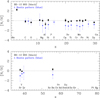 |
Fig. A.4 Chemical pattern of the star BD-12 905 (black), compared to an average pattern of λ Boo stars (blue). |
 |
Fig. A.5 Chemical pattern of the star HD 25674 (black), compared to an average pattern of λ Boo stars (blue). |
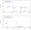 |
Fig. A.6 Chemical pattern of the star HD 36726 (black), compared to an average pattern of λ Boo stars (blue). |
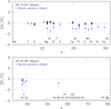 |
Fig. A.7 Chemical pattern of the star HD 37187 (black), compared to an average pattern of λ Boo stars (blue). |
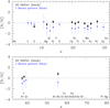 |
Fig. A.8 Chemical pattern of the star HD 290541 (black), compared to an average pattern of λ Boo stars (blue). |
 |
Fig. A.9 Chemical pattern of the star HD 290621 (black), compared to an average pattern of λ Boo stars (blue). |
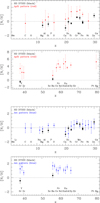 |
Fig. A.10 Chemical pattern of the star HD 37333 (black), compared to an average pattern of Ap stars (upper panels, red lines) and to an average pattern of Am stars (lower panels, blue lines). |
Appendix B Tables of chemical abundances
In this section, we present the chemical abundances derived in this work and their errors. As previously explained, the total error etot was derived as the quadratic sum of the line-to-line dispersion e1 (estimated as ![Mathematical equation: $\[\sigma / \sqrt{n}\]$](/articles/aa/full_html/2025/06/aa54510-25/aa54510-25-eq6.png) , where σ is the standard deviation) and the error in the abundances (e2, e3, and e4) when varying Teff, log g, and vmicro by their corresponding uncertainties8. For chemical species with only one line, we adopted as σ the standard deviation of iron lines. Abundance tables show the average abundance and the total error etot, together with the errors e1 to e4.
, where σ is the standard deviation) and the error in the abundances (e2, e3, and e4) when varying Teff, log g, and vmicro by their corresponding uncertainties8. For chemical species with only one line, we adopted as σ the standard deviation of iron lines. Abundance tables show the average abundance and the total error etot, together with the errors e1 to e4.
Chemical abundances for HD 28548.
Chemical abundances for HD 25674.
Chemical abundances for BD-06 984.
Chemical abundances for BD-08 924.
Chemical abundances for BD-12 905.
Chemical abundances for HD 36726.
Chemical abundances for HD 37333.
Chemical abundances for HD 37187.
Chemical abundances for HD 290541.
Chemical abundances for HD 290621.
Appendix C Average radial velocities and membership
We present in this section the average radial velocities (obtained from our observations and from literature) and membership derived in this work (see Table C.1). The stars included in the list correspond to the initial membership suggested by Hunt & Reffert (2024).
Average radial velocities and membership.
References
- Adams, F. C., Proszkow, E. M., Fatuzzo, M., & Myers, P. C. 2006, ApJ, 641, 504 [NASA ADS] [CrossRef] [Google Scholar]
- Alacoria, J., Saffe, C., Jaque Arancibia, M., et al. 2022, A&A, 660, A98 [NASA ADS] [CrossRef] [EDP Sciences] [Google Scholar]
- Alacoria, J., Saffe, C., Collado, A., et al. 2025, A&A, 696, A123 [NASA ADS] [CrossRef] [EDP Sciences] [Google Scholar]
- Alejo, A. D., González, J. F., & Veramendi, M. E. 2020, A&A, 633, A146 [NASA ADS] [CrossRef] [EDP Sciences] [Google Scholar]
- Andrievsky, S., Chernyshova, I., Paunzen, E., et al. 2002, A&A, 396, 641 [NASA ADS] [CrossRef] [EDP Sciences] [Google Scholar]
- Antoja, T., Figueras, F., Fernández, D., et al. 2008, A&A, 490, 135 [NASA ADS] [CrossRef] [EDP Sciences] [Google Scholar]
- Antoja, T., Figueras, F., & Torra, J. 2010, Lecture Notes and Essays in Astrophysics, 4, Proceedings of the conference held 7–11 September, 2009 at Ciudad Real (Spain), eds. A. Ulla & M. Manteiga (Vigo, Spain: Tórculo Press), 13 [Google Scholar]
- Asplund, M., Grevesse, N., Sauval, A., & Scott, P. 2009, ARA&A, 47, 481 [Google Scholar]
- Bally, J. 2008, Handbook of Star Forming Regions, Volume I: The Northern Sky ASP Monograph Publications, 4, ed. B. Reipurth, 459 [Google Scholar]
- Barros, D., Pérez-Villegas, A., Lépine, J., et al. 2020, ApJ, 888, 75 [NASA ADS] [CrossRef] [Google Scholar]
- Bayo, A., Rodrigo, C., Barrado y Navascués, D., et al. 2008, A&A, 492, 277 [NASA ADS] [CrossRef] [EDP Sciences] [Google Scholar]
- Bertone, E., Buzzoni, A., Chávez, M., et al. 2008, A&A, 485, 823 [NASA ADS] [CrossRef] [EDP Sciences] [Google Scholar]
- Bilir, S., Soydugan, E., Soydugan, F., et al. 2008, AN, 329, 835 [NASA ADS] [Google Scholar]
- Blomme, R., Frémat, Y., Sartoretti, P., et al. 2023, A&A 674, A7 [NASA ADS] [CrossRef] [EDP Sciences] [Google Scholar]
- Bressan, A., Marigo, P., Girardi, L., et al. 2012, MNRAS, 427, 127 [NASA ADS] [CrossRef] [Google Scholar]
- Cahlon, S., Zucker, C., Goodman, A., et al. 2024, ApJ, 961, 153 [NASA ADS] [CrossRef] [Google Scholar]
- Cavallo, L., Spina, L., Carraro, G., et al. 2024, AJ, 167, 12 [NASA ADS] [CrossRef] [Google Scholar]
- Chen, C., Sheehan, P., Watson, D., et al. 2009, ApJ, 701, 1367 [Google Scholar]
- da Silva, L., Girardi, L., Pasquini, L., et al. 2006, A&A, 458, 609 [NASA ADS] [CrossRef] [EDP Sciences] [Google Scholar]
- Dotter, A., Conroy, C., Cargile, P., & Asplund, M. 2017, ApJ, 840, 99 [Google Scholar]
- Draper, Z., Matthews, B., Kennedy, G., et al. 2016, MNRAS, 456, 459 [Google Scholar]
- Faltová, N., Jadlovský, D., Kueb, L., et al. 2025, MNRAS, 536, 72 [Google Scholar]
- Flores, M., Galarza, J., Yana, Miquelarena, P., et al. 2024, MNRAS, 527, 10016 [Google Scholar]
- Gaia Collaboration 2022, VizieR Online Data Catalog, I/357 [Google Scholar]
- Gaia Collaboration (Vallenari, A., et al.) 2023, A&A, 674, A1 [NASA ADS] [CrossRef] [EDP Sciences] [Google Scholar]
- Gagné, J., Faherty, J., Moranta, L., et al. 2021, ApJ, 915, L29 [CrossRef] [Google Scholar]
- Gáspá, A., Su, K., Rieke, G., et al. 2008, ApJ, 672, 974 [Google Scholar]
- Gebran, M., Monier, R., Royer, F., Lobel, A., & Blomme, R. 2014, Putting A Stars into Context: Evolution, Environment, and Related Stars, Proc. of the international conference held on June 3–7, 2013 at Moscow M.V. Lomonosov State Univ., Moscow, Russia, eds. G. Mathys, E. Griffin, O. Kochukhov, R. Monier, & G. Wahlgren (Moscow: Publishing house “Pero”), 193 [Google Scholar]
- González, J. F., & Lapasset, E. 2000, AJ, 119, 2296 [CrossRef] [Google Scholar]
- Gray, R. O., & Corbally, C. J. 1993, AJ, 106, 632 [Google Scholar]
- Gray, R. O., & Corbally, C. J. 1998, AJ, 116, 2530 [NASA ADS] [CrossRef] [Google Scholar]
- Gray, R. O., & Corbally, C. J. 2002, AJ, 124, 989 [NASA ADS] [CrossRef] [Google Scholar]
- Gray, R., Riggs, Q., Koen, C., et al. 2017, AJ, 154, 31 [NASA ADS] [CrossRef] [Google Scholar]
- Heiter, U. 2002, A&A, 381, 959 [NASA ADS] [CrossRef] [EDP Sciences] [Google Scholar]
- Hu, Q., Zhang, Y., Qin, S., et al. 2024, A&A, 687, A291 [NASA ADS] [CrossRef] [EDP Sciences] [Google Scholar]
- Huang, S., Portegies Zwart, S., & Wilhelm, M. 2024, A&A, 689, A338 [NASA ADS] [CrossRef] [EDP Sciences] [Google Scholar]
- Hunt, E., & Reffert, S. 2023, A&A, 673, A114 [NASA ADS] [CrossRef] [EDP Sciences] [Google Scholar]
- Hunt, E., & Reffert, S. 2024, A&A, 686, A42 [NASA ADS] [CrossRef] [EDP Sciences] [Google Scholar]
- Jönsson, H., Holtzman, J. A., Allende Prieto, C., et al. 2020, AJ, 160, 120 [Google Scholar]
- Jura, M., Chen, C., Furlan, E., et al. 2004, ApJSS, 154, 453 [Google Scholar]
- Kamp, I., & Paunzen, E. 2002, MNRAS, 335, L45 [NASA ADS] [CrossRef] [Google Scholar]
- Kamp, I., Iliev, I. Kh., Paunzen, E., et al. 2001, A&A, 375, 899 [NASA ADS] [CrossRef] [EDP Sciences] [Google Scholar]
- Katz, D., Sartoretti, P., Guerrier, A., et al. 2023, A&A, 674, A5 [NASA ADS] [CrossRef] [EDP Sciences] [Google Scholar]
- Kenyon, S., & Hartmann, L. 1995, ApJSS, 101, 117 [Google Scholar]
- Kurucz, R. L. 1993, ATLAS9 Stellar Atmosphere Programs and 2 km/s grid, Kurucz CD-ROM 13 (Cambridge, MA: Smithsonian Astrophysical Obs.) [Google Scholar]
- Kurucz, R. L., & Avrett, E. H. 1981, SAO Special Report No. 391 [Google Scholar]
- Kushniruk, I., Bensby, T., Feltzing, S., et al. 2020, A&A, 638, A154 [NASA ADS] [CrossRef] [EDP Sciences] [Google Scholar]
- Maconi, E., Alves, J., Swiggum, C., et al. 2025, A&A, 694, A167 [NASA ADS] [CrossRef] [EDP Sciences] [Google Scholar]
- Martinez-Galarza, J., Kamp, I., Su, K. Y., et al. 2009, ApJ, 694, 165 [NASA ADS] [CrossRef] [Google Scholar]
- Martos, G., Meléndez, J., Rathsam, A., et al. 2023, MNRAS 522, 3217 [NASA ADS] [CrossRef] [Google Scholar]
- Miquelarena, P., Saffe, C., Flores, M., et al. 2024, A&A, 688, A73 [NASA ADS] [CrossRef] [EDP Sciences] [Google Scholar]
- Morgan, W. W., Keenan, P. C., & Kellman, E. 1943, Atlas of Stellar Spectra (Chicago: University of Chicago Press) [Google Scholar]
- Murphy, S. J., & Paunzen, E. 2017, MNRAS, 466, 546 [NASA ADS] [CrossRef] [Google Scholar]
- Murphy, S., Corbally, C., Gray, R., et al. 2015, PASA, 32, e036 [NASA ADS] [CrossRef] [Google Scholar]
- Murphy, S., Gray, R., Corbally, C., et al. 2020, MNRAS, 499, 2701 [NASA ADS] [CrossRef] [Google Scholar]
- Nguyen, C. T., Costa, G., Girardi, L., et al. 2022 A&A, 665, A126 [NASA ADS] [CrossRef] [EDP Sciences] [Google Scholar]
- Paunzen, E. 2001, A&A, 373, 633 [NASA ADS] [CrossRef] [EDP Sciences] [Google Scholar]
- Paunzen, E., & Gray, R. O. 1997, A&A Suppl. Ser. 126, 407 [Google Scholar]
- Paunzen, E., Kamp, I., Iliev, I. Kh., et al. 1999, A&A, 345, 597 [NASA ADS] [Google Scholar]
- Paunzen, E., Duffee, B., Heiter, U., et al. 2001, A&A, 373, 625 [NASA ADS] [CrossRef] [EDP Sciences] [Google Scholar]
- Paunzen, E., Kamp, I., Weiss, W., & Wiesemeyer, H. 2003a, A&A, 404, 579 [NASA ADS] [CrossRef] [EDP Sciences] [Google Scholar]
- Paunzen, E., Pintado, O., & Maitzen, H. 2003b, A&A 412, 721 [NASA ADS] [CrossRef] [EDP Sciences] [Google Scholar]
- Paunzen, E., Fraga, L., Heiter, U., et al. 2012a, From interacting binaries to exoplanets: essential modeling tools, IAU Proceeding Symposium 282, eds. M. Richards & I. Hubeny, https://doi.org/10.1017/S1743921311027773 [Google Scholar]
- Paunzen, E., Heiter, U., Fraga, L., et al. 2012b, MNRAS, 419, 3604 [NASA ADS] [CrossRef] [Google Scholar]
- Paunzen, E., Netopil, M., Maitzen, H., et al. 2014, A&A, 564, A42 [NASA ADS] [CrossRef] [EDP Sciences] [Google Scholar]
- Rentzsch-Holm, I. 1996, A&A, 312, 966 [NASA ADS] [Google Scholar]
- Saffe, C., & Levato, H. 2014, A&A, 562, 128 [Google Scholar]
- Saffe, C., Jofré, E., Martioli, E., et al. 2017, A&A, 604, L4 [NASA ADS] [CrossRef] [EDP Sciences] [Google Scholar]
- Saffe, C., Flores, M., Miquelarena, P., et al. 2018, A&A, 620, 54 [Google Scholar]
- Saffe, C., Jofré, E., Miquelarena, P., et al. 2019, A&A, 625, 39 [Google Scholar]
- Saffe, C., Miquelarena, P., Alacoria, J., et al. 2020, A&A, 641, 145 [Google Scholar]
- Saffe, C., Miquelarena, P., Alacoria, J., et al. 2021, A&A, 647, A49 [NASA ADS] [CrossRef] [EDP Sciences] [Google Scholar]
- Saffe, C., Alacoria, J., Miquelarena, P., et al. 2022, A&A, 668, A157 [NASA ADS] [CrossRef] [EDP Sciences] [Google Scholar]
- Schlegel, D., Finkbeiner, D. P., & Davis, M. 1998, ApJ, 500, 525 [Google Scholar]
- Sitnova, T., Mashonkina, L., & Ryabchikova, T. 2013, Astron. Lett., 39, 126 [NASA ADS] [CrossRef] [Google Scholar]
- Steinmetz, M., Guiglion, G., McMillan, P. J., et al. 2020, AJ, 160, 83 [NASA ADS] [CrossRef] [Google Scholar]
- Venn, K., & Lambert, D. 1990, ApJ, 363, 234 [Google Scholar]
- Winter, A., & Haworth, T. 2022, EPJP, 137, 1132 [Google Scholar]
- Yang, Y., Zhao, J., Zhang, J., et al. 2021, ApJ, 922, 105 [NASA ADS] [CrossRef] [Google Scholar]
In this work, we use the term “siblings” for stars that belong to the same stellar population.
We adopt a minimum of 0.01 dex for the errors e2, e3, and e4.
All Tables
All Figures
|
Fig. 1 Spectral energy distribution (black circles) and synthetic spectra (blue continuous line) corresponding to the stars HD 28548 and HD 36726 (left and right panels). |
| In the text | |
|
Fig. 2 Observed, synthetic, and difference spectra (black, blue dotted, and magenta lines) for some stars in our sample. |
| In the text | |
|
Fig. 3 Distribution of probable members of the cluster HSC 1640 (gray circles) in different spaces, including the color–magnitude diagram (upper left), position (upper right), proper motion (lower left), and parallax space (lower right). The position of the λ Boo stars is indicated in the plots (blue diamonds). The cluster center is marked in the coordinate space (red plus signs). The best isochrone fit is shown with a red continuous line in the color–magnitude diagram (upper left). |
| In the text | |
|
Fig. 4 Distribution of probable members of the cluster Theia 139 (gray circles) in different spaces, including the color–magnitude diagram (upper left), position (upper right), proper motion (lower left), and parallax space (lower right). The position of the λ Boo stars is indicated in the plots (blue diamonds). The cluster center is marked in the coordinates space (red plus signs). The best isochrone fit is shown with a red continuous line in the color–magnitude diagram (upper left). |
| In the text | |
|
Fig. A.1 Chemical pattern of the star HD 28548 (black), compared to an average pattern of λ Boo stars (blue). |
| In the text | |
|
Fig. A.2 Chemical pattern of the star BD-08 924 (black), compared to an average pattern of Am stars (blue). |
| In the text | |
|
Fig. A.3 Chemical pattern of the star BD-06 984 (black), compared to an average pattern of λ Boo stars (blue). |
| In the text | |
|
Fig. A.4 Chemical pattern of the star BD-12 905 (black), compared to an average pattern of λ Boo stars (blue). |
| In the text | |
|
Fig. A.5 Chemical pattern of the star HD 25674 (black), compared to an average pattern of λ Boo stars (blue). |
| In the text | |
|
Fig. A.6 Chemical pattern of the star HD 36726 (black), compared to an average pattern of λ Boo stars (blue). |
| In the text | |
|
Fig. A.7 Chemical pattern of the star HD 37187 (black), compared to an average pattern of λ Boo stars (blue). |
| In the text | |
|
Fig. A.8 Chemical pattern of the star HD 290541 (black), compared to an average pattern of λ Boo stars (blue). |
| In the text | |
|
Fig. A.9 Chemical pattern of the star HD 290621 (black), compared to an average pattern of λ Boo stars (blue). |
| In the text | |
|
Fig. A.10 Chemical pattern of the star HD 37333 (black), compared to an average pattern of Ap stars (upper panels, red lines) and to an average pattern of Am stars (lower panels, blue lines). |
| In the text | |
Current usage metrics show cumulative count of Article Views (full-text article views including HTML views, PDF and ePub downloads, according to the available data) and Abstracts Views on Vision4Press platform.
Data correspond to usage on the plateform after 2015. The current usage metrics is available 48-96 hours after online publication and is updated daily on week days.
Initial download of the metrics may take a while.