| Issue |
A&A
Volume 698, June 2025
|
|
|---|---|---|
| Article Number | A69 | |
| Number of page(s) | 16 | |
| Section | Numerical methods and codes | |
| DOI | https://doi.org/10.1051/0004-6361/202554028 | |
| Published online | 03 June 2025 | |
DISPATCH methods: An approximate, entropy-based Riemann solver for ideal magnetohydrodynamics
1
Rosseland Centre for Solar Physics, University of Oslo,
PO Box 1029, Blindern,
0315
Oslo,
Norway
2
Institute of Theoretical Astrophysics, University of Oslo,
PO Box 1029, Blindern,
0315
Oslo,
Norway
★ Corresponding author: This email address is being protected from spambots. You need JavaScript enabled to view it.
Received:
4
February
2025
Accepted:
29
March
2025
Abstract
With the advancement of supercomputers, we can now afford simulations with very wide scale ranges. In astrophysical applications – for example simulating solar, stellar and planetary atmospheres, interstellar medium, and so on – physical quantities such as gas pressure, density, temperature, plasma β, and Mach and Reynolds numbers can vary by orders of magnitude. This requires a robust solver, which can deal with a very wide range of conditions and maintain hydrostatic equilibrium where it is applicable. We reformulated a Godunov-type Harten–Lax–van Leer discontinuities (HLLD) approximate Riemann solver that would be suitable for maintaining hydrostatic equilibrium in atmospheric applications in a range of Mach numbers, which represent regimes where kinetic and magnetic energies dominate over thermal energy without any ad hoc corrections. We changed the solver to use entropy instead of total energy as the primary thermodynamic variable in the system of magnetohydrodynamic equations. The entropy is not conserved; it increases when kinetic and magnetic energy are converted to heat, as it should. We propose using an approximate entropy-based Riemann solver as an alternative to already widely used Riemann solver formulations where it might be beneficial. We conducted a series of standard tests with varying conditions and show that the new formulation for the Godunov-type Riemann solver works and is promising.
Key words: hydrodynamics / magnetohydrodynamics (MHD) / shock waves / turbulence / methods: numerical / Sun: atmosphere
© The Authors 2025
 Open Access article, published by EDP Sciences, under the terms of the Creative Commons Attribution License (https://creativecommons.org/licenses/by/4.0), which permits unrestricted use, distribution, and reproduction in any medium, provided the original work is properly cited.
This article is published in open access under the Subscribe to Open model. This email address is being protected from spambots. You need JavaScript enabled to view it. to support open access publication.
1 Introduction
Turbulent magnetised gas is ubiquitous in astrophysics. In a single system (e.g. stellar and planetary atmospheres, the interstellar medium, etc.), physical quantities such as density, gas pressure, entropy, and temperature can vary by orders of magnitude. We now take our closest star, the Sun, as an example. It has several distinct regions. In the core, energy is generated by nuclear fusion and diffused outward by radiation (gamma and X-rays). When the temperature drops sufficiently for ions to recombine, the opacity of the plasma increases and the radiative diffusion can no longer efficiently transport the energy outward, which causes the plasma to start to simmer. Here, the convection zone begins. The convection zone spans roughly 200 Mm and makes up the outer 30% of the solar interior. The mean free path of the photons increases as the density of the plasma decreases with increasing radius, eventually allowing the photons to escape. This is the optical surface that we can observe: the photosphere. Above the photosphere, in the chromosphere, the thermal energy of the gas no longer dominates the total energy budget; plasma β drops below unity, indicating that magnetic pressure becomes higher than the gas pressure; and the gas flows must follow the magnetic-field configuration. Even higher up, the gas temperature suddenly goes back up to millions of degrees Kelvin. The physical quantities, such as density, gas pressure, and temperature, vary by many orders of magnitude from the deep interior all the way up to the outermost parts of the Sun. However, in the convection zone, radially averaged entropy per unit mass is nearly constant. This suggests using entropy as one of the main quantities in solar and stellar simulations is necessary. Numerically maintaining hydrostatic equilibrium is much easier when a quantity varies very little with depth, unlike temperature or internal or total energy. Existing studies have used entropy as a primary thermodynamic variable – for example, works by Popovas et al. (2018, 2019) and Hotta et al. (2022); however, the partial differential equation (PDE) solvers in these works are either very diffuse in low-velocity motions (i.e. Popovas et al. 2018, 2019) or treat entropy as a conservative quantity and do not account for entropy increase in shocks.
With the advent of exascale computing, we are able to run numerical simulations of increasing complexity, either covering a wider range of physical and temporal scales, or including more physics, such as radiative heat transfer, conductivity, chemistry, non-local thermal equilibrium, the generalised Ohm’s law, and so on. A very popular group of tools to solve the equations of magnetohydrodynamics (MHD) is the Godunov-type Riemann solvers. These solvers are efficient in conditions where detailed turbulent structures ought to be preserved, but due to numerical precision cannot accurately evolve thermal energy when kinetic and magnetic energies dominate the energy budget. This can create negative pressure spots in, for example, solar corona; cause inaccurate convective flow velocities; or create areas with negative temperatures in a giant molecular cloud simulation. This is a well-known problem with HLL- and Roe-type Riemann solvers (e.g. Teyssier 2015, Sect. 6.6). Many attempts have been made to mitigate the issue (e.g. Ryu et al. 1993; Bryan et al. 1995; Ismail & Roe 2009; Winters & Gassner 2016; Herbin et al. 2020; Gallice et al. 2022); these did not necessarily resolve the problems, but they at least make them negligible under certain conditions. One alternative to these fixes would be using logarithmic density and pressure.
In this paper, we present a prescription for an approximate entropy-based Riemann solver, which for simplicity we call HLLS. It is based on the Harten-Lax-van Leer discontinuities (HLLD) approximate Riemann solver in RAMSES code (Fromang et al. 2006); see also Miyoshi & Kusano (2005) for a detailed description of an HLLD solver). The HLLS solver is not entropy conserving – shocks and magneto-acoustic waves generate entropy by converting kinetic and magnetic energy to heat. It is an irreversible process. In a closed system, energy cannot be created or destroyed; it can only change its form. This is a fundamental requirement and is mathematically1 fulfilled in total energy-based Riemann solvers. As we are converting the solver to an entropy-based one, we must take into account the entropy increase in shocks and magneto-acoustic waves. In principle, the generated entropy Sgen depends on the state of the Riemann fan and is characterised by the change in primitive quantities – density, velocity, and total pressure – when crossing a given discontinuity. However, in practise, computing entropy production via discontinuities is insufficient. Riemann solvers are diffusive due to the use of slope limiters as well as finite numerical precision. Section 2 briefly covers the key aspects of the HLLD Riemann solver, which are relevant to the discussion of the changes and underlying considerations when converting to an entropy-based solver in Sect. 4. We briefly discuss the equation of state (EOS) where entropy is one of the primary variables and how to compute one in Sect. 3. We continue by showing a few numerical tests in Sect. 5. In Sect. 6, we discuss the current limitations of the solver and the applications, where this solver would be the most beneficial. We conclude by discussing our future development work.
2 The total energy-based HLLD Riemann solver
The ideal MHD equations are a classical system of equations used to study the dynamics of conducting fluids. In traditional Riemann solvers, the fluid equations for the total mass density, momentum density, total energy density, and the magnetic field of the system can be written as a system of conservation laws:
![Mathematical equation: $\[\frac{\partial}{\partial t}\left[\begin{array}{c}\rho \\\rho \boldsymbol{u} \\E_{\mathrm{tot}} \\\boldsymbol{B}\end{array}\right]+\nabla \cdot\left[\begin{array}{c}\rho \boldsymbol{u} \\\rho(\boldsymbol{u} \otimes \boldsymbol{u})+P_{\mathrm{tot}}-\boldsymbol{B} \otimes \boldsymbol{B} \\\boldsymbol{u}\left(E_{\mathrm{tot}}+P_{\mathrm{tot}}\right)-\boldsymbol{B}(\boldsymbol{u} \cdot \boldsymbol{B}) \\\boldsymbol{B} \otimes \boldsymbol{u}-\boldsymbol{u} \otimes \boldsymbol{B}\end{array}\right]=0,\]$](/articles/aa/full_html/2025/06/aa54028-25/aa54028-25-eq1.png) (1)
(1)
with
![Mathematical equation: $\[\nabla \cdot \boldsymbol{B}=0,\]$](/articles/aa/full_html/2025/06/aa54028-25/aa54028-25-eq2.png) (2)
(2)
where ρ, u, Etot, Ptot, and B are density, velocity, total energy, total pressure, and magnetic field, respectively. Total energy is a sum of internal, kinetic, and magnetic energies:
![Mathematical equation: $\[E_{\mathrm{tot}}=\rho \varepsilon+\frac{\rho \boldsymbol{u}^2}{2}+\frac{|\boldsymbol{B}|^2}{2},\]$](/articles/aa/full_html/2025/06/aa54028-25/aa54028-25-eq3.png) (3)
(3)
where ε is internal energy per unit mass and the total pressure, Ptot, is a sum of gas and magnetic pressures:
![Mathematical equation: $\[P_{\mathrm{tot}}=P_{\mathrm{gas}}+\frac{|\boldsymbol{B}|^2}{2}.\]$](/articles/aa/full_html/2025/06/aa54028-25/aa54028-25-eq4.png) (4)
(4)
The system is closed by an EOS. In this work, we used a simple gamma-law (ideal gas) EOS:
![Mathematical equation: $\[P=\rho(\gamma-1) \varepsilon,\]$](/articles/aa/full_html/2025/06/aa54028-25/aa54028-25-eq5.png) (5)
(5)
where γ is the adiabatic index.
The beauty of System (1) lies in the total energy – when one type of energy is converted to another, one does not have to explicitly compute the conversion via, for example, Maxwell stress tensors, Lorentz force, diagonal Reynolds stress, and so on. It saves time and retains very high precision levels, at least in theory. In practice, however, there are complications, mostly due to numerical floating point precision. If magnetic or kinetic energy strongly dominates over thermal energy, the precision of the latter drops to an extent that the expressed pressure or temperature can become negative.
3 The entropy-based equation of state
To define the temperature and entropy, we used an ideal gas law:
![Mathematical equation: $\[P=\frac{\rho k_B T}{\mu m_u},\]$](/articles/aa/full_html/2025/06/aa54028-25/aa54028-25-eq6.png) (6)
(6)
where kB is the Boltzmann constant, μ is the mean molecular weight, T is the gas temperature, and mu is the atomic mass unit. Entropy per unit mass is defined as
![Mathematical equation: $\[S=S_0+c_v ~\ln(P \rho^{-\gamma}),\]$](/articles/aa/full_html/2025/06/aa54028-25/aa54028-25-eq7.png) (7)
(7)
where ![Mathematical equation: $\[c_{v}=\left(\frac{\partial \varepsilon}{\partial T}\right)_{\rho}\]$](/articles/aa/full_html/2025/06/aa54028-25/aa54028-25-eq8.png) is the heat capacity at constant volume. Here, we introduce the entropy null-point S0. It can be considered as an integration constant or the starting point of the summation of the microstates. Having S0 is not necessary (i.e. S0 = 0), and mathematically the entropy value can be both positive and negative, but physically the entropy should not go below 02. From a computational point of view, it is best to keep S as close to zero as possible; then, small gradients in entropy retain the precision.
is the heat capacity at constant volume. Here, we introduce the entropy null-point S0. It can be considered as an integration constant or the starting point of the summation of the microstates. Having S0 is not necessary (i.e. S0 = 0), and mathematically the entropy value can be both positive and negative, but physically the entropy should not go below 02. From a computational point of view, it is best to keep S as close to zero as possible; then, small gradients in entropy retain the precision.
It is really convenient to express Eq. (7) as
![Mathematical equation: $\[S=S_0+\frac{k_B}{(\gamma-1) \mu m_u} ~\ln(P \rho^{-\gamma})=S_0+\frac{\wp}{\gamma-1} ~\ln(P \rho^{-\gamma});\]$](/articles/aa/full_html/2025/06/aa54028-25/aa54028-25-eq9.png) (8)
(8)
here, ![Mathematical equation: $\[\wp=\frac{k_{B}}{\mu m_{u}}=R\]$](/articles/aa/full_html/2025/06/aa54028-25/aa54028-25-eq10.png) , where R is the gas constant. Now we can notice that ℘ repeats itself in both the entropy definition and the ideal gas law. Thus, we can use it as a scaling factor for both temperature and entropy, making the modified entropy,
, where R is the gas constant. Now we can notice that ℘ repeats itself in both the entropy definition and the ideal gas law. Thus, we can use it as a scaling factor for both temperature and entropy, making the modified entropy,
![Mathematical equation: $\[\mathfrak{S}(\gamma-1)=S_0+~ln(P \rho^{-\gamma}),\]$](/articles/aa/full_html/2025/06/aa54028-25/aa54028-25-eq11.png) (9)
(9)
a dimensionless quantity, which is also much closer to unity; thus, numerical operations using it are more accurate. Converting to code units is a common practice in numerical simulations.
Entropy in Eq. (7) represents the thermodynamic concept of entropy, which is a measure of the disorder or randomness of a system. For more realistic gases, entropy per mole can be expressed from total partition sums (e.g. Popovas & Jørgensen 2016, Eq. (43)):
![Mathematical equation: $\[S=R ~\ln~ Q_{\mathrm{tot}}+\frac{R T}{Q_{\mathrm{tot}}}\left(\frac{\partial Q_{\mathrm{tot}}}{\partial T}\right),\]$](/articles/aa/full_html/2025/06/aa54028-25/aa54028-25-eq12.png) (10)
(10)
where Qtot is the total partition sum.
For an arbitrary tabular EOS, entropy can be derived from other quantities by integrating
![Mathematical equation: $\[d S=\left[\frac{1}{T}\left(\frac{\partial \varepsilon}{\partial T}\right)_\rho\right] d T+\left[\frac{1}{T}\left(\frac{\partial \varepsilon}{\partial \ln \rho}\right)_T-\frac{P}{T \rho}\right] d ~\ln~ \rho.\]$](/articles/aa/full_html/2025/06/aa54028-25/aa54028-25-eq13.png) (11)
(11)
The first term in the second brackets on the RHS of Eq. (11) is generally very small, and for ideal gas it vanishes completely, leading to
![Mathematical equation: $\[d S=\left[\frac{1}{T}\left(\frac{\partial \varepsilon}{\partial T}\right)_\rho\right] d T-\left[\frac{P}{T \rho}\right] d ~\ln~ \rho.\]$](/articles/aa/full_html/2025/06/aa54028-25/aa54028-25-eq14.png) (12)
(12)
It is, however, very important to check that the new entropy-based table satisfies Maxwell’s thermodynamic identity,
![Mathematical equation: $\[\left(\frac{\partial \varepsilon}{\partial \rho}\right)_T=\frac{P}{\rho^2}-\frac{T}{\rho^2}\left(\frac{\partial P}{\partial T}\right)_\rho=\frac{P}{\rho^2}\left[\left(\frac{\partial ~\ln~ P}{\partial ~\ln~ T}\right)_\rho\right],\]$](/articles/aa/full_html/2025/06/aa54028-25/aa54028-25-eq15.png) (13)
(13)
and gives exact results to numerical precision for requested quantities, when compared to the original table. In fact, any EOS must satisfy the thermodynamic identity (Eq. 13).
Lastly, sometimes entropy is adopted to be S = Pρ−γ (e.g. Ryu et al. 1993; Canivete Cuissa & Teyssier 2022); this is called modified entropy, which should be considered as a different kind of polytropic EOS and does not have a real physical meaning. Although this quantity could be used as a probe for thermal energy, it does not relate to thermodynamic entropy. On the other hand, it works really well in maintaining thermal energy stability in ideal gases, as shown by Ryu et al. (1993). It is not surprising, since the quantity is advected as a passive scalar, that it will be conserved to numerical precision despite not giving accurate values as to where entropy (or thermal energy in this case) should increase.
4 The conversion to an entropy-based HLLD solver
In the DISPATCH implementation (Nordlund et al. 2018) of this new solver, we used the MUSCL-Hancock algorithm with constrained transport (Evans & Hawley 1988, CT) for the induction equation, as well as a positivity-preserving three-dimensional (3D) unsplit TVD slope limiter (see Fromang et al. (2006) for details). For convenience, do not give full details of the Godunov scheme and we use standard notation. However, we summarize the modified numerical method in Appendix A with the changes depicting the conversion from total energy to entropy. For a deeper overview of HLL, HLLC, and HLLD Riemann solvers, we refer the reader to Miyoshi & Kusano (2005) and Toro (2019), and references therein. The main differences compared to typical HLLD solvers are the parts where total energy is replaced with entropy, with additional fluxes computed to calculate the entropy production (details below).
In the system of equations (1), we replace the total energy term with entropy per unit mass:
![Mathematical equation: $\[\frac{\partial}{\partial t}\left[\begin{array}{c}\rho \\\rho \boldsymbol{u} \\\rho S \\\boldsymbol{B}\end{array}\right]+\nabla \cdot\left[\begin{array}{c}\rho \boldsymbol{u} \\\rho(\boldsymbol{u} \otimes \boldsymbol{u})+P_{\mathrm{tot}}-\boldsymbol{B} \otimes \boldsymbol{B} \\\rho \boldsymbol{u} S \\\boldsymbol{B} \otimes \boldsymbol{u}-\boldsymbol{u} \otimes \boldsymbol{B}\end{array}\right]=\left[\begin{array}{c}0 \\\boldsymbol{\Phi} \\\left(\boldsymbol{Q}_{\mathrm{ext}}+\boldsymbol{Q}_S\right) / T \\0\end{array}\right].\]$](/articles/aa/full_html/2025/06/aa54028-25/aa54028-25-eq16.png) (14)
(14)
For completeness, we also show the additional source terms here, such as Φ, which is the force per unit volume and includes the force of gravity, Coriolis force, and so on. Qext is the external heating per unit volume, which includes Newton cooling, radiative heat transfer, and so on. QS is entropy production from converting kinetic and magnetic energy to heat. The source terms from gravity, Coriolis forces, Newton cooling, and so on are added during both the predictor and the corrector steps.
The system in Eq. (14) can be written in vectorial form, similarly to, for example, Londrillo & Del Zanna (2000):
![Mathematical equation: $\[\frac{\partial \mathbf{U}}{\partial t}+\frac{\partial \mathbf{F}}{\partial x}+\frac{\partial \mathbf{G}}{\partial y}+\frac{\partial \mathbf{H}}{\partial z}=\Psi,\]$](/articles/aa/full_html/2025/06/aa54028-25/aa54028-25-eq17.png) (15)
(15)
where
![Mathematical equation: $\[\mathbf{U}=\left(\rho, \rho {\mathrm{u_x}}, \rho {\mathrm{u_y}}, \rho {\mathrm{u_z}}, \rho \mathrm{S}, {\mathrm{B_x}}, {\mathrm{B_y}}, {\mathrm{B_c}}\right)^{\mathrm{T}},\]$](/articles/aa/full_html/2025/06/aa54028-25/aa54028-25-eq18.png) (16)
(16)
![Mathematical equation: $\[\Psi=\left(0, \Phi_x, \Phi_y, \Phi_z, Q / T+Q_S / T, 0,0,0\right)^T,\]$](/articles/aa/full_html/2025/06/aa54028-25/aa54028-25-eq19.png) (17)
(17)
and
![Mathematical equation: $\[\mathbf{F}=\left(\begin{array}{c}\rho u_x \\\rho u_x^2+P_{t o t}-B_x^2 \\\rho u_x u_y-B_x B_y \\\rho u_x u_z-B_x B_z \\\rho u_x S \\0 \\u_x B_y-u_y B_x \\u_x B_z-u_z B_x\end{array}\right)\]$](/articles/aa/full_html/2025/06/aa54028-25/aa54028-25-eq20.png) (18)
(18)
is the flux function. The expressions for the terms G and H are completely analogous. These equations have seven eigenvalues, corresponding to four magneto-acoustic waves (two slow and two fast), two Alfvén waves, and an entropy wave:
![Mathematical equation: $\[\lambda_{1,7}=u \mp c_f, \quad \lambda_{3,5}=u \mp c_s, \quad \lambda_{2,6}=u \mp c_a, \quad \lambda_4=u,\]$](/articles/aa/full_html/2025/06/aa54028-25/aa54028-25-eq21.png) (19)
(19)
where
![Mathematical equation: $\[c_{f, s}^2=d \pm \sqrt{d^2-a B_x^2 / \rho}, \quad c_a=\frac{\left|B_x\right|}{\sqrt{\rho}}\]$](/articles/aa/full_html/2025/06/aa54028-25/aa54028-25-eq22.png) (20)
(20)
with
![Mathematical equation: $\[d=\frac{a^2+|\boldsymbol{B}|^2 / \rho}{2},\]$](/articles/aa/full_html/2025/06/aa54028-25/aa54028-25-eq23.png) (21)
(21)
and a is the speed of sound. More often than not some eigenvalues in Eq. (19) coincide:
![Mathematical equation: $\[\lambda_1 \leq \lambda_2 \leq \lambda_3 \leq \lambda_4 \leq \lambda_5 \leq \lambda_6,\]$](/articles/aa/full_html/2025/06/aa54028-25/aa54028-25-eq24.png) (22)
(22)
depending on the direction and strength of the magnetic field. A solution to the Riemann problem may thus be composed not only of ordinary shock and rarefaction waves, but also compound waves (Brio & Wu 1988; Miyoshi & Kusano 2005). In the set of equations (18), we do not show the additional fluxes that will be needed to compute the entropy generation, which is discussed in detail below.
4.1 Entropy production
The entropy production in shocks from dissipation of kinetic energy has long been a topic of discussion (Salas & Iollo 1995). Kelvin and Rayleigh questioned the validity of shock discontinuity as it violated the conservation of entropy. A very curious result was put forward by Morduchow & Libby (1949) that equilibrium entropy has a maximum inside a Navier-Stokes shock profile, indicating that entropy was decreasing after passing the shock, strengthening the doubts by Stokes, Kelvin, and Rayleigh. Salas & Iollo (1995) explored this curiosity and concluded that because of this phenomenon, the entropy propagation equation cannot be used as a conservation law. Using a single jump condition for the propagation of entropy is not adequate, as going from equations with two jumps, [P] and [u], to an equation with a single jump, [S], information is lost (see Sect. 5 in Salas & Iollo (1995) for details). Shocks in the infinitesimally small area cannot be considered equilibrium, as the adiabatic index changes locally because of the rapid compression. Rankine–Hugoniot jump conditions are only applicable when elements are far enough from the discontinuity, allowing to assume that the gas is in a local equilibrium on each of the sides. The condition also implies the discontinuity is not resolved. Margolin (2017) studied non-equilibrium entropy in a shock and showed that it increases monotonically inside the shock and a certain modification can be applied to the equilibrium formulation so that it follows the non-equilibrium formulation better. Thornber et al. (2008) derived analytical formulae for the rate of increase of entropy at arbitrary jumps in primitive variables for Godunov methods. It is used later for total energy corrections.
Instead of correcting the total energy, we rewrote the Riemann solver to work in terms of entropy as a primary thermodynamic variable. We can split the evolution of entropy into two parts: the advection of the conserved entropy and new entropy production via the dissipation of kinetic and magnetic energy. The conserved entropy is advected through the Riemann fan as a passive scalar (see Appendix A for details). For the second part, we start by looking at the evolution of total, kinetic, magnetic, and thermal energies. The total energy can be split into its constituent thermal (Eth), kinetic (Ekin) and magnetic (Emag) energies:
![Mathematical equation: $\[E_{\mathrm{tot}}=E_{\mathrm{th}}+E_{\mathrm{kin}}+E_{\mathrm{mag}},\]$](/articles/aa/full_html/2025/06/aa54028-25/aa54028-25-eq25.png) (23)
(23)
while its evolution is thus
![Mathematical equation: $\[\frac{d E_{\mathrm{tot}}}{d t}=\frac{d E_{\mathrm{th}}}{d t}+\frac{d E_{\mathrm{kin}}}{d t}+\frac{d E_{\mathrm{mag}}}{d t}.\]$](/articles/aa/full_html/2025/06/aa54028-25/aa54028-25-eq26.png) (24)
(24)
Since the total energy is conserved, any local change in one form of energy must be accounted for by corresponding fluxes or conversions into other forms. To properly track entropy production, we examine the contributions from kinetic, magnetic, and thermal energies separately:
![Mathematical equation: $\[\frac{d E_{\mathrm{kin}}}{d t}=-\boldsymbol{\nabla} \cdot \mathbf{F}_{\mathrm{kin}}+W_{\mathrm{gas}}-Q_{\mathrm{kin}}+\Theta_{\mathrm{kin}},\]$](/articles/aa/full_html/2025/06/aa54028-25/aa54028-25-eq27.png) (25)
(25)
![Mathematical equation: $\[\frac{d E_{\mathrm{th}}}{d t}=-\boldsymbol{\nabla} \cdot \mathbf{F}_{\mathrm{th}}-W_{\mathrm{gas}}+Q_{\mathrm{kin}}+\Theta_{\mathrm{th}},\]$](/articles/aa/full_html/2025/06/aa54028-25/aa54028-25-eq28.png) (26)
(26)
![Mathematical equation: $\[\frac{d E_{\mathrm{mag}}}{d t}=-\boldsymbol{\nabla} \cdot \mathbf{F}_{\mathrm{mag}}-\Theta_{\mathrm{kin}}-\Theta_{\mathrm{th}},\]$](/articles/aa/full_html/2025/06/aa54028-25/aa54028-25-eq29.png) (27)
(27)
where ∇ · Fkin, ∇ · Fth, and ∇ · Fmag are the kinetic, thermal, and magnetic energy fluxes, respectively; ![Mathematical equation: $\[\frac{d E_{\text {kin }}}{d t}, \frac{d E_{\text {th }}}{d t}\]$](/articles/aa/full_html/2025/06/aa54028-25/aa54028-25-eq30.png) , and
, and ![Mathematical equation: $\[\frac{d E_{\text {mag }}}{d t}\]$](/articles/aa/full_html/2025/06/aa54028-25/aa54028-25-eq31.png) are the change of kinetic, thermal, and magnetic energies in a given cell in a time-step dt. Qkin is heating from kinetic energy dissipation, and Θkin and Θth are conversion of magnetic energy to kinetic and thermal energies, respectively (e.g. reconnection, Ohmic dissipation, etc.). Lastly, Wgas = P(∇ · u) is the pressure work. From Eqs. (25)–(27), we can derive the heating from the irreversible energy dissipation QS = Qkin + Θth:
are the change of kinetic, thermal, and magnetic energies in a given cell in a time-step dt. Qkin is heating from kinetic energy dissipation, and Θkin and Θth are conversion of magnetic energy to kinetic and thermal energies, respectively (e.g. reconnection, Ohmic dissipation, etc.). Lastly, Wgas = P(∇ · u) is the pressure work. From Eqs. (25)–(27), we can derive the heating from the irreversible energy dissipation QS = Qkin + Θth:
![Mathematical equation: $\[\mathbf{Q_{\mathrm{S}}}=-\nabla \cdot \mathbf{F}_{\mathrm{kin}}-\nabla \cdot \mathbf{F}_{\mathrm{mag}}-\frac{d E_{\mathrm{kin}}}{d t}-\frac{d E_{\mathrm{mag}}}{d t}+W_{\mathrm{gas}}.\]$](/articles/aa/full_html/2025/06/aa54028-25/aa54028-25-eq32.png) (28)
(28)
Therefore, to compute QS we need additional quantities from the corrector step: the kinetic and magnetic energy fluxes, as well as the normal velocities at the cell faces to compute ∇ · u. These velocities can be extracted from the corrector step by passing the normal velocity along with the fluxes (see Appendix A for the complete description of the corrector step). To accurately compute QS, a consistent evaluation of the kinetic and magnetic energy time derivatives is needed.
The time derivatives of kinetic and magnetic energy, ![Mathematical equation: $\[\frac{d E_{\text {kin }}}{d t}\]$](/articles/aa/full_html/2025/06/aa54028-25/aa54028-25-eq33.png) and
and ![Mathematical equation: $\[\frac{d E_{\text {mag }}}{d t}\]$](/articles/aa/full_html/2025/06/aa54028-25/aa54028-25-eq34.png) , are computed by evaluating these quantities at both the old (at t) and new (at t + 1) time steps. Specifically, Ekin and Emag are first computed from the conserved variables at the beginning of the time step. Then, after updating the density, momentum, and magnetic fields via flux divergences, the new values of Ekin and Emag are computed. The time derivatives are then approximated as simple finite differences between these two states. This approach ensures consistency with the numerical fluxes and avoids introducing additional diffusive or dispersive errors. Furthermore, this discretisation is fully consistent with the MUSCL-Hancock predictor-corrector scheme used in the solver. If a different time-integration scheme, such as a higher order Runge–Kutta method, were employed, the computation of
, are computed by evaluating these quantities at both the old (at t) and new (at t + 1) time steps. Specifically, Ekin and Emag are first computed from the conserved variables at the beginning of the time step. Then, after updating the density, momentum, and magnetic fields via flux divergences, the new values of Ekin and Emag are computed. The time derivatives are then approximated as simple finite differences between these two states. This approach ensures consistency with the numerical fluxes and avoids introducing additional diffusive or dispersive errors. Furthermore, this discretisation is fully consistent with the MUSCL-Hancock predictor-corrector scheme used in the solver. If a different time-integration scheme, such as a higher order Runge–Kutta method, were employed, the computation of ![Mathematical equation: $\[\frac{d E_{\text {kin }}}{d t}\]$](/articles/aa/full_html/2025/06/aa54028-25/aa54028-25-eq35.png) and
and ![Mathematical equation: $\[\frac{d E_{\text {mag }}}{d t}\]$](/articles/aa/full_html/2025/06/aa54028-25/aa54028-25-eq36.png) would need to be adjusted accordingly to maintain consistency with the chosen temporal discretisation.
would need to be adjusted accordingly to maintain consistency with the chosen temporal discretisation.
This entropy-generation calculation recipe fully accounts for entropy production in shocks and shearing, as well as for numerical dissipation of kinetic and magnetic energy via slope limiters, for example, thus fully closing the system. Lastly, to fully adhere to the second law of thermodynamics, we require QS to be positive-definite:
![Mathematical equation: $\[\frac{\partial(\rho S)}{\partial t}=-\boldsymbol{\nabla} \cdot(\rho \mathbf{u} S)+\max \left(0, \frac{\boldsymbol{Q}_{\mathbf{S}}}{T}\right).\]$](/articles/aa/full_html/2025/06/aa54028-25/aa54028-25-eq37.png) (29)
(29)
4.2 Summary
To reformulate a total-energy-based HLLD Riemann solver, we need to replace the total energy with entropy in both predictor and corrector steps, if the Godunov method is used. Here are the steps:
Replace thermal-energy-based EOSs (Eq. (5)) with entropy-based EOSs (Eq. (8)).
-
In the predictor step, it is sufficient to advect S as a passive scalar to obtain the source term σ, (e.g. for the right state):
![Mathematical equation: $\[\sigma_S=\frac{\Delta t}{2}\left(-\boldsymbol{u} \frac{\partial s}{\partial t}\right) \pm \frac{\Delta \xi}{2}\left(-\boldsymbol{u} \frac{\partial s}{\partial \xi}\right),\]$](/articles/aa/full_html/2025/06/aa54028-25/aa54028-25-eq38.png) (30)
(30)where ξ = [x, y, z] is the spatial dimension.
Compute the Godunov flux for entropy instead of total energy.
Compute the Godunov flux for kinetic and magnetic energies (see Appendix A).
Compute QS using Eq. (28).
Compute the
![Mathematical equation: $\[S_{\text {gen }}=\max \left(0, \frac{Q_{\mathrm{S}}}{T}\right)\]$](/articles/aa/full_html/2025/06/aa54028-25/aa54028-25-eq39.png) .
.Apply Godunov flux, heating
![Mathematical equation: $\[\frac{Q_{\text {ext }}}{T}\]$](/articles/aa/full_html/2025/06/aa54028-25/aa54028-25-eq40.png) and Sgen to obtain St+1.
and Sgen to obtain St+1.
In the next section, we show a number of tests we put this new solver through.
5 The numerical tests
To check the validity of the HLLS solver, we conducted a series of experiments. They are in 1D, 2D, and 3D, and both hydrodynamic and MHD. We ran 1D tests in all principal directions and 2D tests in all three planes to make sure the solver is well balanced in all dimensions. We note that some tests were run on low resolution intentionally, as resolution-starved experiments may reveal problems that are inversely proportional to resolution. The experiments were run in single floating-point precision.
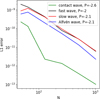 |
Fig. 1 Convergence in norm of L1 error vector for contact, fast, slow, and Alfvén waves after propagating a distance of one wavelength. The convergence rate P is given in the legend. |
5.1 Linear wave convergence
This test shows that the HLLS formulation converges with second-order accuracy for linear amplitude waves. The test is nearly identical to that of Sect. 8.2 in Stone et al. (2008), with a uniform medium where the generic quantities are ![Mathematical equation: $\[\left(\rho, \gamma, P, \mathbf{u}, B_{x}, B_{y}, B_{z}\right)=[1,5 / 3,3 / 5,0,1, \sqrt{2}, 1 / 2]\]$](/articles/aa/full_html/2025/06/aa54028-25/aa54028-25-eq41.png) . The exact eigenfunctions for fast and slow magnetosonic, Alfvén, and contact waves for the background state are given in Gardiner & Stone (2005). Since we usually operate in single floating-point precision, the original wave amplitude of A = 10−6 is too close to the round-off error and is impractical to conduct an informative test. Thus, the only difference compared to Stone et al. (2008) is that we set the wave amplitude value to be A = 10−3. The resulting waves are still weak and do not steepen into shocks. Figure 1 shows the norm of the L1 error vector for each wave family as a function of the numerical resolution from 48 to 1024 cells. The figure shows that we achieve second-order accuracy in both space and time for smooth solutions.
. The exact eigenfunctions for fast and slow magnetosonic, Alfvén, and contact waves for the background state are given in Gardiner & Stone (2005). Since we usually operate in single floating-point precision, the original wave amplitude of A = 10−6 is too close to the round-off error and is impractical to conduct an informative test. Thus, the only difference compared to Stone et al. (2008) is that we set the wave amplitude value to be A = 10−3. The resulting waves are still weak and do not steepen into shocks. Figure 1 shows the norm of the L1 error vector for each wave family as a function of the numerical resolution from 48 to 1024 cells. The figure shows that we achieve second-order accuracy in both space and time for smooth solutions.
5.2 Entropy wave
Riemann solvers are generally very good at preserving shocks. However, very slowly moving waves are sometimes more difficult. To test the diffusion and dispersion error, we launched a very slowly moving discontinuity (entropy wave) in one dimension. Assuming the experiment is carried out in the x direction, the generic quantities are (ρ, P) = [0.9, 1.0] when x < 0 and [1.1, 1.0] when x ≥ 0. All other quantities are set to 0, with ![Mathematical equation: $\[\gamma=\frac{5}{3}\]$](/articles/aa/full_html/2025/06/aa54028-25/aa54028-25-eq42.png) and
and ![Mathematical equation: $\[S=ln (\frac{P}{\rho^{\gamma}}) /(\gamma-1)\]$](/articles/aa/full_html/2025/06/aa54028-25/aa54028-25-eq43.png) in the entire experiment. Boundaries are periodic. We used a rather low resolution of 100 cells in the direction of the wave propagation to exaggerate the dispersion error. The velocity ux of the whole box was set as constant to [1.0, 0.1, 0.01, 0.001, 0.001], and the runtime of the experiment was set to, respectively, tend = [1, 10, 100, 1000, 1000] time units. This means the number of updates increased tenfold with each run. If the solver is diffusive, the wave form should smear out. Figure 2 shows the test results at the end time, when the wave crosses one period. Naturally, the corners are slightly rounded from slope limiters, but we can clearly see that with lower velocities the increase in diffusion is negligible. The diffusion is resolution-sensitive and depends on the slope limiters. The black curve is at time=0, the blue one is at ux = 1, the red one is at ux = 0.1, the dashed green one is at ux = 0.01, and the dotted magenta one is at ux = 0.001. At the lowest velocity, we observe noticeable distortion. This is expected, as many Riemann solvers that are not asymptotic-preserving become excessively diffusive at low Mach numbers. The issue arises because numerical dissipation is often linked to jumps in the velocity component that is normal to the cell interfaces, which do not scale correctly with Mach number. As a result, even small spurious variations in this velocity component can lead to disproportionately large diffusion, particularly when M ≤ 0.2.
in the entire experiment. Boundaries are periodic. We used a rather low resolution of 100 cells in the direction of the wave propagation to exaggerate the dispersion error. The velocity ux of the whole box was set as constant to [1.0, 0.1, 0.01, 0.001, 0.001], and the runtime of the experiment was set to, respectively, tend = [1, 10, 100, 1000, 1000] time units. This means the number of updates increased tenfold with each run. If the solver is diffusive, the wave form should smear out. Figure 2 shows the test results at the end time, when the wave crosses one period. Naturally, the corners are slightly rounded from slope limiters, but we can clearly see that with lower velocities the increase in diffusion is negligible. The diffusion is resolution-sensitive and depends on the slope limiters. The black curve is at time=0, the blue one is at ux = 1, the red one is at ux = 0.1, the dashed green one is at ux = 0.01, and the dotted magenta one is at ux = 0.001. At the lowest velocity, we observe noticeable distortion. This is expected, as many Riemann solvers that are not asymptotic-preserving become excessively diffusive at low Mach numbers. The issue arises because numerical dissipation is often linked to jumps in the velocity component that is normal to the cell interfaces, which do not scale correctly with Mach number. As a result, even small spurious variations in this velocity component can lead to disproportionately large diffusion, particularly when M ≤ 0.2.
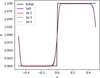 |
Fig. 2 Entropy wave test. Density profiles at starting time (black) and for different wave speeds ux: blue – 1.0, red – 0.1, green dashed – 0.01, magenta dotted – 0.001. The overlap of wave profiles is perfect, with expected slopes present. |
5.3 Shu & Osher shock tube
This test is a 1D Mach=3 shock interacting with sine waves in density (Shu & Osher 1989). It tests the solver’s ability to capture both shocks and small-scale smooth flow. The computational domain is nine length units long and is split into two regions with different conditions in each of them. Assuming the experiment is carried out in the x direction, the quantities are (ρ, ux, P) = [3.857143, 2.629369, 10.33333] when x < −4 and [1 + 0.2 sin (5x), 0,1] when x ≥ −4. All the other quantities are set to 0, with γ = 1.4 and ![Mathematical equation: $\[S=ln (\frac{P}{\rho^{\gamma}}) /(\gamma-1)\]$](/articles/aa/full_html/2025/06/aa54028-25/aa54028-25-eq44.png) in the whole experiment. Figure 3 shows the test results at time = 1.8 time units (red curve). The reference run is done with the HLLD solver (black curve, perfectly covered by the red curve). Both the test and the reference runs had 1500 cells. We additionally show an HLLS run with 500 cells (dots).
in the whole experiment. Figure 3 shows the test results at time = 1.8 time units (red curve). The reference run is done with the HLLD solver (black curve, perfectly covered by the red curve). Both the test and the reference runs had 1500 cells. We additionally show an HLLS run with 500 cells (dots).
5.4 Brio & Wu shock tube
This is a classical test of an MHD shock tube, described by Brio & Wu (1988, Sect. V), where the right and left states are initialised to different values. The left state is initialised as (ρ, ux, uy, uz, By, Bz, P) = [1, 0, 0, 1, 0, 1], and the right state is [0.125, 0, 0, −1, 0, 0.1]. Bx = 0.75 and γ = 2. This test shows whether the solver can accurately represent the shocks, rarefaction waves, compound structures, and contact discontinuities. Figure 4 shows the test results at time = 1.0. The black curve is for a reference HLLD run with 1200 cells. The red curve is for the HLLS run. The blue dots show the HLLS run with 400 cells. Both high- and low-resolution runs overlap each other nearly perfectly and follow the profiles in the literature very accurately. From left to right we can identify a fast rarefaction wave, compound wave, contact discontinuity, slow shock, and a fast rarefaction wave again.
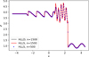 |
Fig. 3 Shu & Osher shock-tube test. Density profile at time=1.8; black: reference HLLD solver with 1500 cells; red: HLLS solver with 1500 cells; blue dots: HLLS solver with 500 cells. |
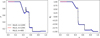 |
Fig. 4 Brio & Wu shock-tube test. Density profile (left) and y component of magnetic field (right) at time=1.0; black: reference HLLD solver with 1200 cells; red: HLLS solver with 1200 cells; blue dots: HLLS solver with 400 cells. Black and red overlap each other nearly perfectly. |
5.5 Kelvin–Helmholtz instability
Kelvin-Helmholtz instability occurs when velocity shear is present within a continuous fluid or across fluid boundaries. We conducted the test as described in McNally et al. (2012). For convenience, here we summarize the setup. The domain is one unit by one unit in the x – and y-directions, with resolutions of 256 × 256 cells. All boundaries are periodic. The density is given by
![Mathematical equation: $\[\rho=\left\{\begin{array}{ll}\rho_1-\rho_m e^{\frac{y-1 / 4}{L}} & \text { if } 1 / 4>\mathrm{y} \geq 0 \\\rho_2+\rho_m e^{\frac{1 / 4-y}{L}} & \text { if } 1 / 2>\mathrm{y} \geq 1 / 4 \\\rho_2+\rho_m e^{-\frac{3 / 4-y}{L}} & \text { if } 3 / 4>\mathrm{y} \geq 1 / 2 \\\rho_1-\rho_m e^{-\frac{y-3 / 4}{L}} & \text { if } 1>\mathrm{y} \geq 3 / 4\end{array},\right.\]$](/articles/aa/full_html/2025/06/aa54028-25/aa54028-25-eq45.png) (31)
(31)
where ρm = (ρ1 − ρ2)/2, ρ1 = 1.0, ρ2 = 2.0 and L = 0.025. The x-direction velocity is given by
![Mathematical equation: $\[u_x=\left\{\begin{array}{ll}u_1-u_m e^{\frac{y-1 / 4}{L}} & \text { if } 1 / 4>\mathrm{y} \geq 0 \\u_2+u_m e^{\frac{1 / 4-y}{L}} & \text { if } 1 / 2>\mathrm{y} \geq 1 / 4 \\u_2+u_m e^{-\frac{3 / 4-y}{L}} & \text { if } 3 / 4>\mathrm{y} \geq 1 / 2 \\u_1-u_m e^{-\frac{y-3 / 4}{L}} & \text { if } 1>\mathrm{y} \geq 3 / 4\end{array},\right.\]$](/articles/aa/full_html/2025/06/aa54028-25/aa54028-25-eq46.png) (32)
(32)
where um = (u1 − u2)/2, u1 = 0.5 and u2 = −0.5. The background shear is perturbed by adding velocity in the y–direction:
![Mathematical equation: $\[u_y=0.01 \sin (4 \pi x).\]$](/articles/aa/full_html/2025/06/aa54028-25/aa54028-25-eq47.png) (33)
(33)
An ideal EOS with γ = 5/3 is used. The initial gas pressure Pgas = 2.5. We ran the simulation until time t = 10. To make an exact comparison to codes in McNally et al. (2012), we show the gas density at t = 1.5 and the maximal value of vertical kinetic energy evolution in time in Figure 5. We note that we used 256 × 256 resolution, but the result is directly comparable to the 5122 and 40962 runs in McNally et al. (2012). In the right panel of the figure, we show the maximum value of vertical kinetic energy in the simulation for three resolutions. From this figure, it can be seen that primary instability begins at exactly the same time. Secondary instabilities occur around the same time as well, indicating that we obtain a converged solution even at the low resolution of 256 × 256.
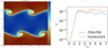 |
Fig. 5 HD Kelvin-Helmholtz instability. Density profile (left) and time evolution of kinetic energy (right). |
5.6 Rayleigh–Taylor instability
Another classic test of a code’s ability to handle subsonic perturbations is the Rayleigh–Taylor instability, which has been described in a number of studies (e.g. Stone & Gardiner 2007; Abel 2011; Hopkins 2015). In this test, a layer of heavier fluid is placed on top of a layer of lighter fluid. With gravitational source term added to the forces, we test two things: whether the explicit addition of force is correct, and the solver’s ability to preserve instabilities while keeping things symmetric at the right time; that is, during the linear phase. During the nonlinear phase, in a sufficiently high resolution the symmetry is expected to break by construction. We used the initial setup similar to those of Abel (2011) and Hopkins (2015). Here, we recap the setup for convenience. In a two-dimensional domain with 0 ≤ x ≤ 0.5 (128 cells for low-resolution runs and 768 for high-resolution runs) and 0 ≤ y ≤ 1 (256 and 1536 cells for low- and high-resolution runs, respectively), we used periodic boundary conditions in the x direction and constant boundary conditions in the y direction. In this test, we used γ = 1.4, and the density profile was initialised as ρ(y) = ρ1 + (ρ2 − ρ1)/(1 + e−(y−0.5)/Δ), where ρ1 = 1 and ρ2 = 2 are the density below and above the contact discontinuity (yc, respectively, with Δ = 0.025 being its width). The pressure gradient is in hydrostatic equilibrium with a uniform gravitational acceleration of g = −0.5 in the y direction, P = ρ2/γ + g ρ(y) (y − yc), and then entropy S = (ln(P) − ln(ρ)γ)/(γ − 1). An initial y-velocity perturbation vy = δvy(1 + cos(8π(x + 0.25)))(1 + cos (5π(y − 0.5))) with δvy = 0.025 is applied in the 0.3 ≤ y ≤ 0.7 range (Hopkins 2015).
Figure 6 shows the evolution of the instability at different times. The initial velocity grows, and the heavier fluid starts to sink. We note the single-cell resolution of contact discontinuities and mixing. Both blobs are perfectly symmetric during the linear phase. Soon enough, Kelvin-Helmholtz instabilities develop at the shear surface between the fluids, and the symmetry is harder to maintain due to low relative velocities. However, the low-resolution run maintained perfect symmetry throughout the whole simulation. Figure 7 shows the high-resolution run. Secondary instabilities are more pronounced, and thus the symmetry is harder to maintain. The figure can be directly compared to Fig. 22 in Hopkins (2015). Our high-resolution (768 × 1536) run shows very similar features to those of Hopkins (2015), although we maintain much better symmetries until the blobs reach the bottom.
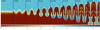 |
Fig. 6 Rayleigh–Taylor instability in low (128 × 256) resolution. We plot density at different times. |
5.7 ‘Hot-bubble’ experiment
To evaluate the entropy-preserving properties of our numerical scheme in a strongly stratified, low Mach-number regime, we performed the hot-bubble test following the setup of Edelmann et al. (2021). This experiment simulates the buoyant rise of a localised entropy perturbation embedded in an isentropic but highly stratified layer. In stellar interiors, entropy fluctuations drive convection; however, outside the heating or cooling layers these fluctuations should remain conserved, except for mixing effects. Maintaining accurate entropy advection in such conditions is usually numerically challenging due to the large variations in pressure and density. The experimental setup is identical to the original, with resolution of 128 × 192 cells in the x- and y-directions. The gravitational acceleration is then
![Mathematical equation: $\[g_z=g_0 ~\sin (k_z z),\]$](/articles/aa/full_html/2025/06/aa54028-25/aa54028-25-eq48.png) (34)
(34)
where g0 = −1.099044 × 105 cm and kz = 2π/zmax, zmax = 1.5 × 106 cm, while xmax is 1 × 106 cm. γ = 5/3, at z = 0 P0 = 106 Ba, with temperature T0 = 300 K. The stratification is isentropic; that is,
![Mathematical equation: $\[\rho(z)=\left(\frac{P(z)}{A}\right)^{1 / \gamma},\]$](/articles/aa/full_html/2025/06/aa54028-25/aa54028-25-eq49.png) (35)
(35)
where A = A0 = const everywhere outside of the bubble. As the A0 value is not given in Edelmann et al. (2021), we used the ideal gas EOS to obtain ρ0 = P/RgasT = 4.00906 × 10⁻⁵ and consequently A0 = 2.129425 × 10¹³. A = P/ργ is not a true entropy expression, as discussed in Sect. 3, but a rather good probe for it. Since ideal gas entropy can be simplified to S = ln(P/ργ)/(γ − 1), we can express S = S0 = ln(A)/(γ − 1) = 46.03419. The hydrostatic pressure stratification is given by
![Mathematical equation: $\[P(z)=\left[P_0^{1-\frac{1}{\gamma}}+\left(1-\frac{1}{\gamma}\right) \frac{g_0}{A_0^{\frac{1}{\gamma}} k_z}\left[1-\cos \left(k_z z\right)\right]\right]^{\frac{\gamma}{\gamma-1}},\]$](/articles/aa/full_html/2025/06/aa54028-25/aa54028-25-eq50.png) (36)
(36)
which is not perturbed and has a low-to-high ratio of 100. The perturbation is only applied for density via
![Mathematical equation: $\[A=A_0\left[1+\left(\frac{\Delta A}{A}\right)_{t=0} \cos \left(\frac{\pi r}{2 r_0}\right)^2\right],\]$](/articles/aa/full_html/2025/06/aa54028-25/aa54028-25-eq51.png) (37)
(37)
where (ΔA/A)t=0 = 10−3 is the bubble’s amplitude and r = [(x − x0)2 + (y − y0)2] is the distance from the bubble’s center. The radius of the bubble is r0 = 1.25 × 105 cm. This low perturbation makes the bubble rise at low Mach numbers: a few times 10−2 (Edelmann et al. 2021). To improve the numerical precision, we rescale the length scale, lsc = 105, and density scale, dsc = 4 × 10⁻⁵ leaving the timescale intact. This results in velocities and density, and entropy closer to unity, which in turn leads to the highest numerical accuracy. Since we considered the normalised fluctuations in A, ΔA/A, the scaling does not change the result. The simulation was run from time t = 0 to t = 300 s. Two time slices at t=150 and 300 s are shown in Fig. 8. This figure can be directly compared to Fig. 6 in Edelmann et al. (2021). The HLLS solver performs almost as well as a well-balanced scheme and noticeably better than simulations with energy as the primary thermodynamic variable without any well-balanced schemes. We note that the main challenge for us is the perturbation being very close to the numerical noise limit, as we normally operate with single precision. The adherence to the second law of thermodynamics is ensured to the numerical precision via Eq. (29); thus, the negative entropy and, consequently, A values are from numerical round-off errors.
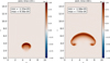 |
Fig. 8 ‘Hot-bubble’ experiment at time=150 and 300 s. Both panels show fluctuations of ΔA/A, with the min/max values given in the floating box. |
5.8 MHD blast
This is a very popular test, and various papers have presented results with slightly different problem setups. It is a very good test of the code’s ability to handle the evolution of strong MHD waves and look for directional biases. We chose to follow the setups of Ramsey et al. (2012), Clarke (2010), and Stone et al. (2008). A rectangular domain with −0.5 ≤ [x, y] ≤ 0.5, 512 × 512 cell resolution was used. All boundaries are periodic. The MHD quantities are set to (ρ, u, Bx, By, Bz) = ![Mathematical equation: $\[(1,0,5 \sqrt{2}, 5 \sqrt{2}, 0)\]$](/articles/aa/full_html/2025/06/aa54028-25/aa54028-25-eq52.png) . The ambient pressure Pgas = 1 with Pgas = 100 within the radius r = 0.125. Figure 9 shows the density and magnetic pressure in the experiment at time t = 0.021 and can be directly compared to Ramsey et al. (2012), Clarke (2010), and Stone et al. (2008). The shock front is sharp, a fast magneto-acoustic wave is travelling at the correct speed, and the blast is symmetric.
. The ambient pressure Pgas = 1 with Pgas = 100 within the radius r = 0.125. Figure 9 shows the density and magnetic pressure in the experiment at time t = 0.021 and can be directly compared to Ramsey et al. (2012), Clarke (2010), and Stone et al. (2008). The shock front is sharp, a fast magneto-acoustic wave is travelling at the correct speed, and the blast is symmetric.
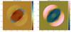 |
Fig. 9 MHD blast experiment. Density (left) and magnetic pressure (right) at time=0.021. We note the sharp shock-fronts. |
5.9 Orszag-Tang vortex
This test has become a staple for MHD codes. The initial setup is identical to those of Stone et al. (2008), and Ramsey et al. (2012). A rectangular domain with −0.5 ≤ [x, y] ≤ 0.5, 1024 × 1024 cells for a high-resolution run is used. All boundaries are periodic. Initially, the pressure and density were constant: Pgas = 5/12π and ρ = 25/36π. The ratio of specific heats γ = 5/3. The initial velocity (ux, uy, uz) = (− sin (2πy), sin (2πx), 0), and the magnetic field was set through the vector potential
![Mathematical equation: $\[A_z=\frac{B_0}{4 \pi} ~\cos (4 \pi x)+\frac{B_0}{2 \pi} ~\cos (4 \pi y),\]$](/articles/aa/full_html/2025/06/aa54028-25/aa54028-25-eq53.png)
where ![Mathematical equation: $\[B_{0}=1 / \sqrt{4 \pi}\]$](/articles/aa/full_html/2025/06/aa54028-25/aa54028-25-eq54.png) . Figures 10 and 11 show density, entropy per unit mass, and magnetic pressure at two times: t = 0.5 and t = 0.75. The t = 0.5 is the typical time this test is shown in literature. When compared to Stone et al. (2008) and Ramsey et al. (2012), we can recognize similar features. We note the very sharp features and perfect symmetry between sides. When advancing the simulation further, the vortex starts producing plasmoids. Here, it is very difficult to maintain symmetry, but the lower panels show that plasmoids are released rather symmetrically.
. Figures 10 and 11 show density, entropy per unit mass, and magnetic pressure at two times: t = 0.5 and t = 0.75. The t = 0.5 is the typical time this test is shown in literature. When compared to Stone et al. (2008) and Ramsey et al. (2012), we can recognize similar features. We note the very sharp features and perfect symmetry between sides. When advancing the simulation further, the vortex starts producing plasmoids. Here, it is very difficult to maintain symmetry, but the lower panels show that plasmoids are released rather symmetrically.
This experiment is very effective in testing the solver stability. In high resolution, discontinuities and rarefactions are more severe, and Riemann solvers can crash from negative pressure or thermal energy values if they cannot deal with them. Since we have an HLLD solver that can also use both total and thermal energies as an available primary thermodynamic variable, we can investigate the conservation of different quantities in different formulations. Figure 12 shows the time evolution of horizontally averaged kinetic (top left), magnetic (bottom right), internal (top middle), and total (top middle) energies, as well as density (bottom left) and entropy (bottom middle). The resolution was identical in all the runs (256 × 256). HLLS represents the run with the solver (presented in this paper), and HLLS-2 allows QS to be negative, breaking the second law of thermodynamics, but more accurately following the energy dissipation and numerical dispersion (see discussion in Sect. 6.1); HLLD is a classical HLLD solver where total energy is conserved and magnetic fields are updated using the CT method, but no adjustments are made to the total energy. While HLLD CT is a modification of said solver, where the magnetic-energy contribution in the total energy is updated with the values from CT solver, making it more stable in areas where magnetic energy strongly dominates over kinetic energy. This correction makes the solver not conserve the total energy in favor of conserving all three energies separately.
In the figure, we can see that the HLLS solver does not conserve the total energy, by construction. However, if we allow QS < 0, it tracks the total energy-conserving HLLD solver rather closely, indicating where the second law of thermodynamics is broken in the HLLD solver. The primary reason for this non-conservation is the discrepancy of magnetic fields between the 1D Riemann solver and the CT 2D solver. The former is more diffusive and assumes a normal magnetic field is constant across the interface, while the latter is much less diffusive and preserves ∇ · B = 0 better. Secondary effects stem from numerical dispersion.
The discrepancy between the solvers diminishes with higher resolution. In realistic simulations, open boundary conditions, external forces, and a higher desired resolution may deem the discrepancies in total energy negligible.
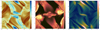 |
Fig. 10 Orszag-Tang vortex test at time = 0.5. Density (left), entropy per unit mass (middle), and magnetic pressure (right). |
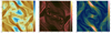 |
Fig. 11 Orszag-Tang vortex test at time = 0.75. Density (left), entropy per unit mass (middle), and magnetic pressure (right). We note the plasmoids forming. |
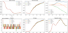 |
Fig. 12 Current-sheet test at different times. Density (top) and magnetic pressure (bottom). |
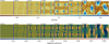 |
Fig. 13 Current-sheet test at different times. Density (top) and magnetic pressure (bottom). |
5.10 Current sheet
The current sheet test problem is designed to determine what an algorithm will do with a perturbed current sheet. Although an analytic solution for this test problem is not available, it is still suitable for testing the robustness of the algorithm. The experimental setup is similar to that of Hawley & Stone (1995). The test is run in two dimensions using a periodic square grid with −0.5 ≤ [x, y] ≤ 0.5 and 256 × 256 cell resolution. There is a uniform magnetic field that discontinuously reverses direction at a certain point. In the whole box (ρ, Pgas) = (1, β/2, where β is an input parameter. We set By:
![Mathematical equation: $\[B_y=\left\{\begin{array}{ll}1 / \sqrt{(4 \pi)} & \text { if }|\mathrm{x}|>0.25 \\-1 / \sqrt{(4 \pi)} & \text { if }|\mathrm{x}| \leq 0.25\end{array}.\right.\]$](/articles/aa/full_html/2025/06/aa54028-25/aa54028-25-eq55.png) (38)
(38)
For |x| > 0.25, velocities (ux, uy) = (A sin (2πy), 0), where A is an amplitude. We ran the test with a range of β and A values, but here we present it only with the “standard” setup, where β = A = 0.1. In Fig. 13 we can see the density and magnetic pressure at different times. Initially linearly polarised Alfvén waves propagate along the field in the y-direction and quickly start generating magneto-acoustic waves since the magnetic pressure does not remain constant. As there are two current sheets in the setup (at x = ±0.25), reconnection inevitably occurs. If β < 1, this reconnection drives strong over-pressurised regions that launch magneto-acoustic waves transverse to the field. Moreover, as reconnection changes the topology of the field lines, magnetic islands form, grow, and merge. The point of the test is to make sure the algorithm can follow this evolution for as long as possible without crashing. We ran tests for 0.1 ≤ (β, A) ≤ 10, and the HLLS solver did not encounter any numerical problems.
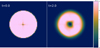 |
Fig. 14 Magnetic-loop advection experiment. The initial magnetic pressure (left) and after the loop has been advected around the grid twice. |
5.11 Magnetic-field loop advection
This is a very powerful test to check whether the scheme preserves ∇ · B = 0. The experiment is similar to those of Tóth & Odstrčil (1996) and Stone et al. (2008) with a two-dimensional domain, 0 ≤ x ≤ 2 (128 cells), and 0 ≤ y ≤ 1 (64 cells). Boundaries are periodic in the whole domain. In this test, γ = 5/3 and both density and gas pressure are constant throughout the box: ρ = Pgas = 1.0. The magnetic field is initialised using a vector potential Az = max [A * (r0 − r), 0], with A = 10−3 and r0 = 0.3, and r is the radial distance from the domain center. The flow velocity (ux, uy) = (2, 1); thus, the problem is essentially an advection test for the vector potential.
Although this test does not test the HLLS solver directly, the CT scheme is nevertheless an integral part of the solver. Moreover, we found this test to be a particularly useful tool to find errors in the magnetic-field predictor step. Figure 14 shows the initial magnetic pressure and that after the magnetic loop has been advected twice through the domain. The shape of the loop is rather well preserved.
 |
Fig. 15 Gresho vortex test. The initial setup (left) and after two rotation periods with different Mach numbers: Ma = 0.1, 0.01, 0.001. The rightmost panel is for a higher resolution run (see text for more details). |
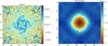 |
Fig. 16 Gas density (left) and pressure (right) in the Gresho vortex test with Ma = 0.01. We note that the quantities are within the noise limit. |
5.12 Gresho vortex
The Gresho vortex is a time-independent rotation pattern. Angular velocity depends only on the radius, and centrifugal force is balanced by the pressure gradient. We used the slightly modified initial condition, which permits the variation of the Mach number; it can be found in Happenhofer et al. (2013) and Grimm-Strele et al. (2014). For convenience, the setup is summarised here. The simulation is in two dimensions − 0 ≤ x ≤ 1 (48 cells) and 0 ≤ y ≤ 1 (48 cells) – with periodic boundary conditions everywhere. The low resolution is deliberate; from our tests, we see that with higher resolution (e.g. Grimm-Strele et al. 2014) the experiment becomes much less challenging to the solver. In the whole domain, ρ = 1, γ = 5/3,
![Mathematical equation: $\[u_\phi= \begin{cases}5 r & \text { if } 0 \leq \mathrm{r}<0.2 \\ 2-5 r & \text { if } 0.2 \leq \mathrm{r} \leq 0.4, ~and \\ 0 & \text { if } 0.4<\mathrm{r}\end{cases}\]$](/articles/aa/full_html/2025/06/aa54028-25/aa54028-25-eq56.png) (39)
(39)
![Mathematical equation: $\[P_{\text {gas }}=\left\{\begin{array}{l}P_0+\frac{25}{2} r^2 \quad \text { if } 0 \leq \mathrm{r}<0.2 \\P_0+\frac{25}{2} r^2+4(1-5 r-\ln (0.2 r) \text { if } 0.2 \leq \mathrm{r} \leq 0.4, \\P_0-2+4 ~\ln (2) \quad \text { if } 0.4<\mathrm{r}\end{array}\right.\]$](/articles/aa/full_html/2025/06/aa54028-25/aa54028-25-eq57.png) (40)
(40)
where ![Mathematical equation: $\[r=\sqrt{\left(x^{2}+y^{2}\right)}\]$](/articles/aa/full_html/2025/06/aa54028-25/aa54028-25-eq58.png) is the radial distance from the center of the domain, uϕ is the angular velocity in terms of the polar angle ϕ = atan2(y, x), and
is the radial distance from the center of the domain, uϕ is the angular velocity in terms of the polar angle ϕ = atan2(y, x), and
![Mathematical equation: $\[P_0=\frac{\rho}{\gamma \mathrm{Ma}_{\mathrm{ref}}^2},\]$](/articles/aa/full_html/2025/06/aa54028-25/aa54028-25-eq59.png) (41)
(41)
with Maref being a reference Mach number, which is the highest Mach number in the resulting flow. Four runs were executed, with Maref = [0.1, 0.01, 0.001]. The last Maref is repeated in two runs at the nominal resolution and a higher resolution, with 128 × 128 cells. Figure 15 shows the results. We deliberately did not run the experiment with higher Mach numbers, as those are just too easy to maintain and the final result looks identical to the initial condition. In the figure, we can see that the vortex is maintained very well down to Ma=0.01. With Ma=0.001, we have the expected outcome; that is, the Godunov-type Riemann solvers deal with very low Mach numbers poorly, even though the Ma=0.01 result is still very good and especially since we used single floating point precision. Figure 16 shows the gas density and pressure with Ma=0.01. It can be clearly seen that the vortex itself is barely distinguishable inside the noise of the box. On the other hand, with increased resolution, the result with Ma=0.001 (as expected) has significantly improved, and the vortex can be once again identified.
5.13 Magnetic rotor
The magnetic rotor tests the propagation of strong torsional Alfén waves as well as solver behavior in moderately high Mach numbers (Ma = 20). A dense disc of fluid rotates within a static fluid background, with a gradual velocity-tapering layer between the disc edge and the ambient fluid. An initially uniform magnetic field is present, which is twisted with the disc rotation. The magnetic field is strong enough that it wraps around the rotor, diminishing the rotor’s angular momentum. The increased magnetic pressure around the rotor compresses the fluid in the rotor, giving it an oblong shape. The experimental setup is introduced by Balsara & Spicer (1999), but we used a more stringent variant of it from Guillet et al. (2019), which is summarised below.
The simulation is in a two-dimensional square, 0 ≤ x, y ≤ 1 (512 × 512 cells), with periodic boundary conditions everywhere. The gas pressure and magnetic fields are uniform in the whole domain, with Pgas = 1, γ = 1.4 and ![Mathematical equation: $\[\mathbf{B}=(5 / \sqrt{4 \pi}, 0,0)\]$](/articles/aa/full_html/2025/06/aa54028-25/aa54028-25-eq60.png) . The gas density is
. The gas density is
![Mathematical equation: $\[\rho= \begin{cases}10 & \text { if } \mathrm{r}<\mathrm{r}_0 \\ 1+9 f & \text { if } \mathrm{r}_0 \leq \mathrm{r} \leq \mathrm{r}_1 \\ 1 & \text { if } \mathrm{r}_1<\mathrm{r}\end{cases},\]$](/articles/aa/full_html/2025/06/aa54028-25/aa54028-25-eq61.png) (42)
(42)
where r0 = 0.1, r1 = 0.115, r is the radial distance from the center of the box c, and f = (r1 − r)/(r1 − r0) is the tapering function for the taper region between the disc and the background. The velocities are
![Mathematical equation: $\[\left(u_x, u_y\right)= \begin{cases}\left(\frac{v_0(c-y)}{r_0}, \frac{v_0(x-c)}{r_0}\right) & \text { if } \mathrm{r}<\mathrm{r}_0 \\ \left(f \frac{v_0(c-y)}{r_0}, f \frac{v_0(x-c)}{r_0}\right) & \text { if } \mathrm{r}_0 \leq \mathrm{r} \leq \mathrm{r}_1 \\ (0,0) & \text { if } \mathrm{r}_1<\mathrm{r}\end{cases},\]$](/articles/aa/full_html/2025/06/aa54028-25/aa54028-25-eq62.png) (43)
(43)
with v0 = 2. The experiment was run until time t = 0.15, by which point the torsional Alfvén waves have almost reached the boundary. Figure 17 shows the density ρ, magnetic pressure PB, Mach number, and normalised magnetic-field divergence ![Mathematical equation: $\[\frac{(\nabla \cdot \mathbf{B}) \Delta x}{|\mathbf{B}|}\]$](/articles/aa/full_html/2025/06/aa54028-25/aa54028-25-eq63.png) . We can note the very sharp details with no distortions outside the now almond-shaped disc. In the compressed areas, the Mach number becomes very high, but it does not pose any issues. The magnetic field is divergence-free within the noise level.
. We can note the very sharp details with no distortions outside the now almond-shaped disc. In the compressed areas, the Mach number becomes very high, but it does not pose any issues. The magnetic field is divergence-free within the noise level.
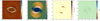 |
Fig. 17 Magnetic rotor test. From left to right: Density, magnetic pressure, Mach number, and |
![Mathematical equation: $\[\frac{\nabla \cdot \mathbf{B}}{|\mathbf{B}|}\]$](/articles/aa/full_html/2025/06/aa54028-25/aa54028-25-eq64.png)
6 Discussion and conclusions
In this paper, we present a new approximate entropy-based HLLD Riemann solver. It works well in both sub- and supersonic regimes and preserves positive temperature and gas pressure. The numerical tests are very encouraging and indicate that the HLLS solver can be readily used in a wide range of physical conditions and experimental setups.
6.1 Considerations about QS being positive-definite
Even though we require QS to be positive-definite, in reality some numerical dispersion and diffusion might artificially increase kinetic or magnetic energy, which in turn breaks total energy conservation if a corresponding decrease in thermal energy does not occur. Indeed, this is one of the main reasons many Riemann solvers fail in conditions where kinetic or magnetic energy strongly dominate over thermal energy: the numerical precision of the latter is reduced if it is several orders of magnitude smaller than the other total energy components, and it can lead to negative thermal energy. In the Orszag-Tang test, described in the Sect. 5.9, we did check the difference; that is, whether the requirement of QS being positive-definite is upheld or not. Until time ≈0.3, the difference is non-existent (indicating that numerical dispersion would not artificially decrease the thermal energy in a total energy solver); however, later we do observe considerable differences. This difference could sometimes be decisive of whether the experiment crashes or not when total or thermal energy is used as a primary thermodynamic variable.
6.2 Very low-Mach-number regimes
The numerical tests show that the HLLS solver can easily handle Mach numbers as low as 0.01, and with lower values it becomes rather diffusive. Of course, the perturbations at such Mach numbers are on the order of numerical precision (see the Gresho vortex in Sect. 5.12 for details) and can be absolutely indistinguishable from the background. This is very encouraging, as Godunov- and Roe-type Riemann solvers with singular precision usually struggle with Mach numbers below 0.1. Various good attempts have been made to modify solvers to reach very low Mach numbers, including those adding correction terms to star states – for example, Shima & Kitamura (2011), Dellacherie et al. (2016), Minoshima & Miyoshi (2021), and Sheng Chen et al. (2022) – or by using well-balanced schemes. In the latter, a hydrostatic equilibrium is imposed directly in the set of dynamic equations, separating primitive variables into equilibrium (stationary) states and dynamical perturbations, as was done in, for example, Greenberg & Leroux (1996), Hotta et al. (2022), and Canivete Cuissa & Teyssier (2022). This approach is less successful and is not as flexible as the first option, although it is indispensable in modelling deep atmospheres as it helps with hydrostatic equilibrium. The numerical precision is better when only perturbations are considered, and there is nothing really preventing gas in incompressible state from acting as compressible gas and ignoring the rotational flows. However, these methods are not mutually exclusive. In fact, combining low-dissipation solvers with well-balancing schemes, as shown by Edelmann et al. (2021), can be particularly effective for modelling highly subsonic flows in strongly stratified media (such as deep stellar convection) while keeping grid sizes reasonably small. Our initial attempts to use a simple ad hoc modification of u⋆ and ![Mathematical equation: $\[P_{\text {tot }}^{\star}\]$](/articles/aa/full_html/2025/06/aa54028-25/aa54028-25-eq65.png) to imitate the transition to incompressible gas at around Mach = 0.2, as in Minoshima & Miyoshi (2021), did not result in any significant improvement; on the contrary, the test experiments produced highly undesirable results. For example, the Gresho vortex, presented in Sect. 5.12, had background gas rotating in the opposite direction. Clearly we need to do more work to balance out the equations if we want to use this method and later expand the formulation to use some form of well-balanced scheme.
to imitate the transition to incompressible gas at around Mach = 0.2, as in Minoshima & Miyoshi (2021), did not result in any significant improvement; on the contrary, the test experiments produced highly undesirable results. For example, the Gresho vortex, presented in Sect. 5.12, had background gas rotating in the opposite direction. Clearly we need to do more work to balance out the equations if we want to use this method and later expand the formulation to use some form of well-balanced scheme.
Lastly, developing a fully 3D wave model for strongly interacting states, akin to the approach in Balsara (2015), is an avenue we would like to explore in the future. While our current HLLS scheme is inherently three-dimensional and unsplit, it still relies on one-dimensional Riemann problems along coordinate-aligned directions. Extending this to a truly multi-dimensional Riemann solver, incorporating a strongly interacting state that evolves self-similarly and enforces consistency with the full three-dimensional conservation laws would enable a more isotropic propagation of flow features and improved treatment of entropy generation from irreversible kinetic and magnetic energy dissipation. This would be particularly beneficial in MHD turbulence and low-Mach-number flows, where current schemes may suffer from excessive numerical dissipation or directional bias. However, significant work is required to implement such a model, including designing a suitable three-dimensional wave structure and computing numerical fluxes that maintain consistency across multiple interacting Riemann problems. We will continue our work on very low Mach-number regimes, as this is rather crucial to the applications we intend to use the solver for.
6.3 Applications
The solver was developed with the primary intent to use it in the context of solar, stellar, and planetary atmospheres. From the outermost regions, towards the cores, density, temperature, and pressure vary by orders of magnitude, but entropy per unit mass stays almost constant. Additionally, HLLS is the preferred solver in situations where magnetic energy and kinetic energy strongly dominate over thermal energy (e.g. the solar chromosphere and corona).
In strongly stratified media, evolving volumetric entropy rather than volumetric energy as a primary variable ensures that entropy gradients, which drive convection, are captured with more accuracy. This is particularly beneficial in nearly isentropic convection zones, where traditional total-energy-based schemes struggle due to the small thermal energy contrast relative to the total energy. However, even in sub-adiabatic regions, where entropy gradients are stable and convection is suppressed, the proposed method remains reliable. Since entropy is a logarithmic quantity by nature, its variability in sub-adiabatic regions does not span orders of magnitude, making it a well-conditioned variable for numerical evolution. This helps maintain accuracy in regions where the entropy contrast is small. For internal gravity waves, entropy-based formulations should naturally capture buoyancy oscillations, as entropy perturbations directly relate to restoring forces in a stratified medium. However, the very low Mach numbers typical of sub-adiabatic regions introduce additional numerical challenges, as discussed above.
We are already employing this solver to simulate the whole solar convective region from 0.655 to 0.998 R⊙ (Popovas et al. in prep.), and we can see that the HLLS solver can maintain the hydrostatic equilibrium much better than an HLLD solver without introducing a well-balanced scheme, as in Edelmann et al. (2021) and Canivete Cuissa & Teyssier (2022), for example.
6.4 Future work
We will keep developing the solver so that it can eventually cover a larger range of Mach numbers and generally perform better. We will consider the following:
solver modifications for very low Mach-number regimes;
implementing a well-balanced scheme consistent with the solver;
solver modifications for relativistic regimes;
heavy optimisation to improve memory alignment and vectorisation that would be also suitable for modern GPUs;
non-ideal MHD effects introducing entropy generation in Ohmic dissipation and ambipolar diffusion.
Acknowledgements
This research was supported by the Research Council of Norway through its Centres of Excellence scheme, project number 262622, and through grants of computing time from the Programme for Supercomputing, as well as through the Synergy Grant number 810218 (ERC-2018-SyG) of the European Research Council. Lastly, we are grateful to the anonymous referee for in-depth review, detailed and insightful comments, and useful suggestions, that significantly improved the manuscript.
Appendix A The numerical method
In Godunov-type schemes the volume-averaged conservative physical quantities at a next time-step are given by integrating an approximate solution to the Riemann problem with left and right states, UL and UR at the cell interface. An HLL Rieman solver (Harten et al. 1983) is constructed by assuming an average intermediate state between the fastest and slowest waves. The information is lost, as slow magneto-acoustic waves are merged together with Alfvén and entropy waves. An HLLC Toro et al. (1994) solver expands and estimates the middle wave of the contact surface. Lastly, HLLD Miyoshi & Kusano (2005) expands into four intermediate states. We start with computing the HLL wave speed. Usually the wave speeds are notated by SL and SR, but to avoid the confusion with entropy, we will note them with ΣL and ΣR:
![Mathematical equation: $\[\begin{aligned}\Sigma_L & =\min \left(u_l, u_r\right)-\max \left(c_{f, l}, c_{f, r}\right) \\\Sigma_R & =\max \left(u_l, u_r\right)+\max \left(c_{f, l}, c_{f, r}\right)\end{aligned}\]$](/articles/aa/full_html/2025/06/aa54028-25/aa54028-25-eq66.png) (A.1)
(A.1)
For convenience, we compute (u · B), which to avoid confusion we denote ϕ, kinetic energy Ekin and magnetic energy Emag for left and right states as well:
![Mathematical equation: $\[\phi_l=u_l A+v_l B_l+w_l C_l,\]$](/articles/aa/full_html/2025/06/aa54028-25/aa54028-25-eq67.png) (A.2)
(A.2)
![Mathematical equation: $\[E_{\mathrm{kin}, l}=\frac{\rho_l}{2}\left(u_l^2+v_l^2+w_l^2\right),\]$](/articles/aa/full_html/2025/06/aa54028-25/aa54028-25-eq68.png) (A.3)
(A.3)
![Mathematical equation: $\[E_{\mathrm{mag}, l}=\frac{1}{2}\left(A^2+B_l^2+C_l^2\right),\]$](/articles/aa/full_html/2025/06/aa54028-25/aa54028-25-eq69.png) (A.4)
(A.4)
and
![Mathematical equation: $\[\phi_r=u_r A+v_r B_r+w_r C_r,\]$](/articles/aa/full_html/2025/06/aa54028-25/aa54028-25-eq70.png) (A.5)
(A.5)
![Mathematical equation: $\[E_{k i n, r}=\frac{\rho_r}{2}\left(u_r^2+v_r^2+w_r^2\right),\]$](/articles/aa/full_html/2025/06/aa54028-25/aa54028-25-eq71.png) (A.6)
(A.6)
![Mathematical equation: $\[E_{m a g, r}=\frac{1}{2}\left(A^2+B_r^2+C_r^2\right).\]$](/articles/aa/full_html/2025/06/aa54028-25/aa54028-25-eq72.png) (A.7)
(A.7)
We define the Lagrangian sound speed,
![Mathematical equation: $\[\begin{aligned}v_L & =u_l-\Sigma_L \\v_R & =\Sigma_R-u_r\end{aligned}\]$](/articles/aa/full_html/2025/06/aa54028-25/aa54028-25-eq73.png) (A.8)
(A.8)
and then compute the acoustic star state:
![Mathematical equation: $\[u^{\star}=\frac{\rho_r u_r v_R+\rho_l u_l v_L+\left(P_{\mathrm{tot}, l}-P_{\mathrm{tot}, r}\right)}{\rho_l v_L+\rho_r v_R}\]$](/articles/aa/full_html/2025/06/aa54028-25/aa54028-25-eq74.png) (A.9)
(A.9)
![Mathematical equation: $\[P_{\mathrm{tot}}^{\star}=\frac{\rho_r v_R P_{\mathrm{tot}, l}+\rho_l v_l P_{\mathrm{tot}, r}+\rho_r \rho_l v_R v_L\left(u_l-u_r\right)}{\rho_l v_L+\rho_r v_R}.\]$](/articles/aa/full_html/2025/06/aa54028-25/aa54028-25-eq75.png) (A.10)
(A.10)
The left star region variables are
![Mathematical equation: $\[\rho_L^{\star}=-\frac{\rho_l v_L}{\Sigma_L-u^{\star}},\]$](/articles/aa/full_html/2025/06/aa54028-25/aa54028-25-eq76.png) (A.11)
(A.11)
![Mathematical equation: $\[v_l^{\star}=\frac{v_l-A B_l\left(u^{\star}-u_l\right)}{e_l^{\star}},\]$](/articles/aa/full_html/2025/06/aa54028-25/aa54028-25-eq77.png) (A.12)
(A.12)
![Mathematical equation: $\[w_l^{\star}=\frac{w_l-A C_l\left(u^{\star}-u_l\right)}{e_l^{\star}},\]$](/articles/aa/full_html/2025/06/aa54028-25/aa54028-25-eq78.png) (A.13)
(A.13)
![Mathematical equation: $\[B_l^{\star}=\frac{B_l e_l}{e_l^{\star}},\]$](/articles/aa/full_html/2025/06/aa54028-25/aa54028-25-eq79.png) (A.14)
(A.14)
![Mathematical equation: $\[C_l^{\star}=\frac{C_l e_l}{e_l^{\star}},\]$](/articles/aa/full_html/2025/06/aa54028-25/aa54028-25-eq80.png) (A.15)
(A.15)
where vl and wl are left tangential velocities, A = Al = Ar is the normal component of the magnetic field, Bl and Cl are the left states of the tangential components of the magnetic field,
![Mathematical equation: $\[e_l^{\star}=-\frac{\rho_l v_L}{\Sigma_L-u^{\star}}-A^2,\]$](/articles/aa/full_html/2025/06/aa54028-25/aa54028-25-eq81.png) (A.16)
(A.16)
and
![Mathematical equation: $\[e_l=-\frac{\rho_l v_L}{\Sigma_L-u_l}-A^2.\]$](/articles/aa/full_html/2025/06/aa54028-25/aa54028-25-eq82.png) (A.17)
(A.17)
Entropy is updated as a passive scalar:
![Mathematical equation: $\[S_l^{\star}=S_l \frac{\rho_l}{\rho_l^{\star}} \frac{-v_L}{\Sigma_L-u^{\star}}.\]$](/articles/aa/full_html/2025/06/aa54028-25/aa54028-25-eq83.png) (A.18)
(A.18)
Left state Alfvén wave speed is
![Mathematical equation: $\[\Sigma_{a, l}=u^{\star}+\frac{|A|}{\sqrt{\rho_l^{\star}}}.\]$](/articles/aa/full_html/2025/06/aa54028-25/aa54028-25-eq84.png) (A.19)
(A.19)
Left star region (u · B), Ekin and Emag are
![Mathematical equation: $\[\phi_l^{\star}=u^{\star} A+v_l^{\star} B_l^{\star}+w_l^{\star} C_l^{\star},\]$](/articles/aa/full_html/2025/06/aa54028-25/aa54028-25-eq85.png) (A.20)
(A.20)
![Mathematical equation: $\[E_{\mathrm{kin}, l}^{\star}=\frac{\rho_l^{\star}}{2}\left(u^{\star 2}+v_l^{\star 2}+w_l^{\star 2}\right),\]$](/articles/aa/full_html/2025/06/aa54028-25/aa54028-25-eq86.png) (A.21)
(A.21)
![Mathematical equation: $\[E_{\mathrm{mag}, l}^{\star}=\frac{1}{2}\left(A^2+B_l^{\star 2}+C_l^{\star 2}\right).\]$](/articles/aa/full_html/2025/06/aa54028-25/aa54028-25-eq87.png) (A.22)
(A.22)
Correspondingly, the right star region variables are:
![Mathematical equation: $\[\rho_r^{\star}=-\frac{\rho_r v_r}{\Sigma_R-u^{\star}},\]$](/articles/aa/full_html/2025/06/aa54028-25/aa54028-25-eq88.png) (A.23)
(A.23)
![Mathematical equation: $\[v_r^{\star}=\frac{v_r-A B_r\left(u^{\star}-u_r\right)}{e_r^{\star}},\]$](/articles/aa/full_html/2025/06/aa54028-25/aa54028-25-eq89.png) (A.24)
(A.24)
![Mathematical equation: $\[w_r^{\star}=\frac{w_r-A C_r\left(u^{\star}-u_r\right)}{e_r^{\star}},\]$](/articles/aa/full_html/2025/06/aa54028-25/aa54028-25-eq90.png) (A.25)
(A.25)
![Mathematical equation: $\[B_r^{\star}=\frac{B_r e_r}{e_r^{\star}},\]$](/articles/aa/full_html/2025/06/aa54028-25/aa54028-25-eq91.png) (A.26)
(A.26)
![Mathematical equation: $\[C_r^{\star}=\frac{C_r e_r}{e_r^{\star}},\]$](/articles/aa/full_html/2025/06/aa54028-25/aa54028-25-eq92.png) (A.27)
(A.27)
where vr and wr are right tangential velocities, A is the normal component of the magnetic field, Br and Cr are the tangential components of the magnetic field,
![Mathematical equation: $\[e_r^{\star}=-\frac{\rho_r v_R}{\Sigma_R-u^{\star}}-A^2,\]$](/articles/aa/full_html/2025/06/aa54028-25/aa54028-25-eq93.png) (A.28)
(A.28)
and
![Mathematical equation: $\[e_r=-\frac{\rho_r v_R}{\Sigma_R-u_l}-A^2.\]$](/articles/aa/full_html/2025/06/aa54028-25/aa54028-25-eq94.png) (A.29)
(A.29)
![Mathematical equation: $\[S_r^{\star}=S_r \frac{\rho_r}{\rho_r^{\star}} \frac{-v_r}{\Sigma_R-u^{\star}}.\]$](/articles/aa/full_html/2025/06/aa54028-25/aa54028-25-eq95.png) (A.30)
(A.30)
Right state Alfvén wave speed is
![Mathematical equation: $\[\Sigma_{a, r}=u^{\star}+\frac{|A|}{\sqrt{\rho_r^{\star}}}.\]$](/articles/aa/full_html/2025/06/aa54028-25/aa54028-25-eq96.png) (A.31)
(A.31)
Right star region (u · B), Ekin and Emag are
![Mathematical equation: $\[\phi_r^{\star}=u^{\star} A+v_r^{\star} B_r^{\star}+w_r^{\star} C_r^{\star},\]$](/articles/aa/full_html/2025/06/aa54028-25/aa54028-25-eq97.png) (A.32)
(A.32)
![Mathematical equation: $\[E_{\mathrm{kin}, r}^{\star}=\frac{\rho_r^{\star}}{2}\left(u^{\star 2}+v_r^{\star 2}+w_r^{\star 2}\right),\]$](/articles/aa/full_html/2025/06/aa54028-25/aa54028-25-eq98.png) (A.33)
(A.33)
![Mathematical equation: $\[E_{\mathrm{mag}, r}^{\star}=\frac{1}{2}\left(A^2+B_r^{\star 2}+C_r^{\star 2}\right).\]$](/articles/aa/full_html/2025/06/aa54028-25/aa54028-25-eq99.png) (A.34)
(A.34)
Lastly, the double star region variables are:
![Mathematical equation: $\[v^{\star \star}=\frac{v_l^{\star} \sqrt{\rho_l^{\star}}+v_r^{\star} \sqrt{\rho_r^{\star}}+\Xi\left(B_r^{\star}-B_l^{\star}\right)}{\sqrt{\rho_l^{\star}}+\sqrt{\rho_r^{\star}}},\]$](/articles/aa/full_html/2025/06/aa54028-25/aa54028-25-eq100.png) (A.35)
(A.35)
![Mathematical equation: $\[w^{\star \star}=\frac{w_l^{\star} \sqrt{\rho_l^{\star}}+w_r^{\star} \sqrt{\rho_r^{\star}}+\Xi\left(C_r^{\star}-C_l^{\star}\right)}{\sqrt{\rho_l^{\star}}+\sqrt{\rho_r^{\star}}},\]$](/articles/aa/full_html/2025/06/aa54028-25/aa54028-25-eq101.png) (A.36)
(A.36)
![Mathematical equation: $\[B^{\star \star}=\frac{B_r^{\star} \sqrt{\rho_l^{\star}}+B_l^{\star} \sqrt{\rho_r^{\star}}+\Xi \sqrt{\rho_l^{\star}} \sqrt{\rho_r^{\star}}\left(v_r^{\star}-v_l^{\star}\right)}{\sqrt{\rho_l^{\star}}+\sqrt{\rho_r^{\star}}},\]$](/articles/aa/full_html/2025/06/aa54028-25/aa54028-25-eq102.png) (A.37)
(A.37)
![Mathematical equation: $\[C^{\star \star}=\frac{C_r^{\star} \sqrt{\rho_l^{\star}}+C_l^{\star} \sqrt{\rho_r^{\star}}+\Xi \sqrt{\rho_l^{\star}} \sqrt{\rho_r^{\star}}\left(w_r^{\star}-w_l^{\star}\right)}{\sqrt{\rho_l^{\star}}+\sqrt{\rho_r^{\star}}},\]$](/articles/aa/full_html/2025/06/aa54028-25/aa54028-25-eq103.png) (A.38)
(A.38)
where Ξ is a sign function, Ξ = sign(A). Note, that there is no double star variable for entropy. Then double star region (u · B) and Emag are
![Mathematical equation: $\[\phi^{\star \star}=u^{\star} A+v^{\star \star} B^{\star \star}+w^{\star \star} C^{\star \star},\]$](/articles/aa/full_html/2025/06/aa54028-25/aa54028-25-eq104.png) (A.39)
(A.39)
![Mathematical equation: $\[E_{\text {mag }}^{\star \star}=\frac{1}{2}\left(A^2+B^{\star \star 2}+C^{\star \star 2}\right).\]$](/articles/aa/full_html/2025/06/aa54028-25/aa54028-25-eq105.png) (A.40)
(A.40)
while left and right double star regions for Ekin are correspondingly
![Mathematical equation: $\[E_{\mathrm{kin}, l}^{\star \star}=\frac{\rho_l^{\star}}{2}\left(u^{\star 2}+v^{\star \star 2}+w^{\star \star 2}\right)\]$](/articles/aa/full_html/2025/06/aa54028-25/aa54028-25-eq106.png) (A.41)
(A.41)
and
![Mathematical equation: $\[E_{\mathrm{kin}, r}^{\star \star}=\frac{\rho_r^{\star}}{2}\left(u^{\star 2}+v^{\star \star 2}+w^{\star \star 2}\right).\]$](/articles/aa/full_html/2025/06/aa54028-25/aa54028-25-eq107.png) (A.42)
(A.42)
A.1 Godunov fluxes
The fluxes are then given by
![Mathematical equation: $\[\boldsymbol{F}_{\mathrm{HLLS}}=\left\{\begin{array}{ll}\boldsymbol{F}_L, & \text { if } \Sigma_{\mathrm{L}}>0 \\\boldsymbol{F}_L^{\star}, & \text { if } \Sigma_{\mathrm{L}} \leq 0 \leq \Sigma_{\mathrm{a}, 1} \\\boldsymbol{F}_L^{\star \star}, & \text { if } \Sigma_{\mathrm{a}, 1} \leq 0 \text { and } \mathrm{u}^{\star}>0 \\\boldsymbol{F}_R^{\star \star}, & \text { if } \mathrm{u}^{\star} \leq 0 \text { and } \Sigma_{\mathrm{a}, \mathrm{r}}>0 \\\boldsymbol{F}_R^{\star}, & \text { if } \Sigma_{\mathrm{a}, \mathrm{r}} \leq 0 \leq \Sigma_{\mathrm{R}} \\\boldsymbol{F}_R, & \text { if } \Sigma_{\mathrm{R}}<0\end{array},\right.\]$](/articles/aa/full_html/2025/06/aa54028-25/aa54028-25-eq108.png) (A.43)
(A.43)
where
![Mathematical equation: $\[\boldsymbol{F}_L=\left(\begin{array}{l}\rho_l u_l \\\rho_l u_l^2+P_{\text {tot, } l}-A^2 \\\rho_l u_l v_l-A B_l \\\rho_l u_l w_l-A C_l \\\rho_l u_l S_l \\0 \\u_l B_l-A v_l \\u_l C_l-A w_l \\u_l\left(E_{\text {kin }, l}+P_{\text {tot, } l}\right) \\u_l E_{\text {mag }, l}-A \phi_l \\u_l\end{array}\right)\]$](/articles/aa/full_html/2025/06/aa54028-25/aa54028-25-eq109.png) (A.44)
(A.44)
![Mathematical equation: $\[\boldsymbol{F}_L^{\star}=\left(\begin{array}{l}\rho_l^{\star} u^{\star} \\\rho_l^{\star} u^{\star 2}+P_{t o t}^{\star}-A^2 \\\rho_l^{\star} u^{\star} v_l^{\star}-A B_l^{\star} \\\rho_l^{\star} u^{\star} w_l^{\star}-A C_l^{\star} \\\rho_l^{\star} u^{\star} S_l^{\star} \\0 \\u^{\star} B_l^{\star}-A v_l^{\star} \\u^{\star} C_l^{\star}-A w_l^{\star} \\u^{\star}\left(E_{k i n, l}^{\star}+P_{t o t}^{\star}\right) \\u^{\star} E_{m a g, l}^{\star}-A \phi_l^{\star} \\u^{\star}\end{array}\right)\]$](/articles/aa/full_html/2025/06/aa54028-25/aa54028-25-eq110.png) (A.45)
(A.45)
![Mathematical equation: $\[F_L^{\star \star}=\left(\begin{array}{l}\rho_l^{\star} u^{\star} \\\rho_l^{\star} u^{\star 2}+P_{t o t}^{\star}-A^2 \\\rho_l^{\star} u^{\star} u^{\star \star}-A B^{\star \star} \\\rho_l^{\star} u^{\star} w^{\star \star}-A C^{\star \star} \\\rho_l^{\star} u^{\star} S_l^{\star} \\0 \\u^{\star} B^{\star \star}-A v^{\star \star} \\u^{\star} C^{\star \star}-A w^{\star \star} \\u^{\star}\left(E_{k i n, l}^{\star \star}+P_{tot}^{\star}\right) \\u^{\star} E_{mag}^{\star \star}-A \phi^{\star \star} \\u^{\star}\end{array}\right)\]$](/articles/aa/full_html/2025/06/aa54028-25/aa54028-25-eq111.png) (A.46)
(A.46)
![Mathematical equation: $\[F_R^{\star \star}=\left(\begin{array}{l}\rho_r^{\star} u^{\star} \\\rho_r^{\star} u^{\star 2}+P_{t o t}^{\star}-A^2 \\\rho_r^{\star} u^{\star} u^{\star \star}-A B^{\star \star} \\\rho_r^{\star} u^{\star} w^{\star \star}-A C^{\star \star} \\\rho_r^{\star} u^{\star} S_r^{\star} \\0 \\u^{\star} B^{\star \star}-A v^{\star \star} \\u^{\star} C^{\star \star}-A w^{\star \star} \\u^{\star}\left(E_{kin, r}^{\star \star}+P_{tot}^{\star}\right) \\u^{\star} E_{mag}^{\star \star}-A \phi^{\star \star} \\u^{\star}\end{array}\right)\]$](/articles/aa/full_html/2025/06/aa54028-25/aa54028-25-eq112.png) (A.47)
(A.47)
![Mathematical equation: $\[\boldsymbol{F}_R^{\star}=\left(\begin{array}{l}\rho_r^{\star} u^{\star} \\\rho_r^{\star} u^{\star 2}+P_{tot}^{\star}-A^2 \\\rho_r^{\star} u^{\star} v_r^{\star}-A B_r^{\star} \\\rho_r^{\star} u^{\star} w_r^{\star}-A C_r^{\star} \\\rho_r^{\star} u^{\star} S_r^{\star} \\0 \\u^{\star} B_r^{\star}-A v_r^{\star} \\u^{\star} C_r^{\star}-A w_r^{\star} \\u^{\star}\left(E_{kin,r}^{\star}+P_{tot}^{\star}\right) \\u^{\star} E_{mag,r}^{\star}-A \phi_r^{\star} \\u^{\star}\end{array}\right)\]$](/articles/aa/full_html/2025/06/aa54028-25/aa54028-25-eq113.png) (A.48)
(A.48)
![Mathematical equation: $\[\boldsymbol{F}_R=\left(\begin{array}{l}\rho_r u_r \\\rho_r u_r^2+P_{t o t, r}-A^2 \\\rho_r u_r v_r-A B_r \\\rho_r u_r w_r-A C_r \\\rho_r u_r S_r \\0 \\u_r B_r-A v_r \\u_r C_r-A w_r \\u_r\left(E_{k i n, r}+P_{t o t, r}\right) \\u_r E_{m a g, r}-A \phi_r \\u_r\end{array}\right)\]$](/articles/aa/full_html/2025/06/aa54028-25/aa54028-25-eq114.png) (A.49)
(A.49)
In the brackets above there are these Godunov fluxes:
density flux
normal momentum flux
first tangential velocity flux
second tangential velocity flux
entropy flux
normal magnetic field component flux
first tangential magnetic field component flux
second tangential magnetic field component flux
kinetic energy flux
magnetic energy flux
normal velocity
Magnetic field component fluxes are used to update the magnetic fields in order to get the ![Mathematical equation: $\[\frac{d E_{\text {mag }}}{d t}\]$](/articles/aa/full_html/2025/06/aa54028-25/aa54028-25-eq115.png) . If CT method is used to update the magnetic fields, this step is still necessary for consistency (temporarily storing
. If CT method is used to update the magnetic fields, this step is still necessary for consistency (temporarily storing ![Mathematical equation: $\[\frac{d E_{\text {mag }}}{d t}\]$](/articles/aa/full_html/2025/06/aa54028-25/aa54028-25-eq116.png) separately), as the actual magnetic field update is done through the electromotive force from the cell edges. The kinetic and magnetic energy fluxes are used to compute ∇ · Fkin and ∇ · Fmag respectively, while normal velocity (last item) is used to compute P (∇ · u) to get the gas pressure work Wgas.
separately), as the actual magnetic field update is done through the electromotive force from the cell edges. The kinetic and magnetic energy fluxes are used to compute ∇ · Fkin and ∇ · Fmag respectively, while normal velocity (last item) is used to compute P (∇ · u) to get the gas pressure work Wgas.
References
- Abel, T. 2011, MNRAS, 413, 271 [Google Scholar]
- Balsara, D. S. 2015, J. Computat. Phys., 295, 1 [Google Scholar]
- Balsara, D. S., & Spicer, D. S. 1999, J. Computat. Phys., 149, 270 [Google Scholar]
- Brio, M., & Wu, C. 1988, J. Computat. Phys., 75, 400 [Google Scholar]
- Bryan, G. L., Norman, M. L., Stone, J. M., Cen, R., & Ostriker, J. P. 1995, Comput. Phys. Commun., 89, 149 [Google Scholar]
- Canivete Cuissa, J. R., & Teyssier, R. 2022, A&A, 664, A24 [Google Scholar]
- Clarke, D. A. 2010, ApJS, 187, 119 [NASA ADS] [CrossRef] [Google Scholar]
- Dellacherie, S., Jung, J., Omnes, P., & Raviart, P.-A. 2016, Math. Models Methods Appl. Sci., 26, 2525 [Google Scholar]
- Edelmann, P. V. F., Horst, L., Berberich, J. P., et al. 2021, A&A, 652, A53 [NASA ADS] [CrossRef] [EDP Sciences] [Google Scholar]
- Evans, C. R., & Hawley, J. F. 1988, ApJ, 332, 659 [Google Scholar]
- Fromang, S., Hennebelle, P., & Teyssier, R. 2006, A&A, 457, 371 [NASA ADS] [CrossRef] [EDP Sciences] [Google Scholar]
- Gallice, G., Chan, A., Loubère, R., & Maire, P.-H. 2022, J. Computat. Phys., 468, 111493 [Google Scholar]
- Gardiner, T. A., & Stone, J. M. 2005, J. Computat. Phys., 205, 509 [Google Scholar]
- Greenberg, J. M., & Leroux, A. Y. 1996, SIAM J. Numer. Anal., 33, 1 [Google Scholar]
- Grimm-Strele, H., Kupka, F., & Muthsam, H. 2014, Comput. Phys. Commun., 185, 764 [Google Scholar]
- Guillet, T., Pakmor, R., Springel, V., Chandrashekar, P., & Klingenberg, C. 2019, MNRAS, 485, 4209 [Google Scholar]
- Happenhofer, N., Grimm-Strele, H., Kupka, F., Löw-Baselli, B., & Muthsam, H. 2013, J. Computat. Phys., 236, 96 [Google Scholar]
- Harten, A., Lax, P. D., & Leer, B. V. 1983, SIAM Rev., 25, 35 [Google Scholar]
- Hawley, J. F., & Stone, J. M. 1995, Comput. Phys. Commun., 89, 127 [NASA ADS] [CrossRef] [Google Scholar]
- Herbin, R., Latché, J.-C., & Zaza, C. 2020, IMA J. Numer. Anal., 40, 1792 [CrossRef] [MathSciNet] [Google Scholar]
- Hopkins, P. F. 2015, MNRAS, 450, 53 [Google Scholar]
- Hotta, H., Kusano, K., & Shimada, R. 2022, ApJ, 933, 199 [NASA ADS] [CrossRef] [Google Scholar]
- Ismail, F., & Roe, P. L. 2009, J. Computat. Phys., 228, 5410 [Google Scholar]
- Londrillo, P., & Del Zanna, L. 2000, ApJ, 530, 508 [NASA ADS] [CrossRef] [Google Scholar]
- Margolin, L. 2017, Entropy, 19 [Google Scholar]
- McNally, C. P., Lyra, W., & Passy, J.-C. 2012, ApJS, 201, 18 [NASA ADS] [CrossRef] [Google Scholar]
- Minoshima, T., & Miyoshi, T. 2021, J. Computat. Phys., 446, 110639 [NASA ADS] [CrossRef] [Google Scholar]
- Miyoshi, T., & Kusano, K. 2005, J. Computat. Phys., 208, 315 [NASA ADS] [CrossRef] [Google Scholar]
- Morduchow, M., & Libby, P. A. 1949, J. Aeronaut. Sci., 16, 674 [Google Scholar]
- Nordlund, Å., Ramsey, J. P., Popovas, A., & Küffmeier, M. 2018, MNRAS, 477, 624 [NASA ADS] [CrossRef] [Google Scholar]
- Popovas, A., & Jørgensen, U. G. 2016, A&A, 595, A130 [NASA ADS] [CrossRef] [EDP Sciences] [Google Scholar]
- Popovas, A., Nordlund, Å., Ramsey, J. P., & Ormel, C. W. 2018, MNRAS, 479, 5136 [Google Scholar]
- Popovas, A., Nordlund, Å., & Ramsey, J. P. 2019, MNRAS, 482, L107 [NASA ADS] [CrossRef] [Google Scholar]
- Ramsey, J. P., Clarke, D. A., & Men’shchikov, A. B. 2012, ApJS, 199, 13 [Google Scholar]
- Ryu, D., Ostriker, J. P., Kang, H., & Cen, R. 1993, ApJ, 414, 1 [Google Scholar]
- Salas, M. D., & Iollo, A. 1995, Entropy jump across an inviscid shock wave, Final Report (Hampton, VA: Institute for Computer Applications in Science and Engineering) [Google Scholar]
- Sheng Chen, S., Ping Li, J., Li, Z., Yuan, W., & Hong Gao, Z. 2022, J. Computat. Phys., 456, 111027 [Google Scholar]
- Shima, E., & Kitamura, K. 2011, AIAA J., 49, 1693 [Google Scholar]
- Shu, C.-W., & Osher, S. 1989, J. Computat. Phys., 83, 32 [Google Scholar]
- Stone, J. M., & Gardiner, T. 2007, ApJ, 671, 1726 [NASA ADS] [CrossRef] [Google Scholar]
- Stone, J. M., Gardiner, T. A., Teuben, P., Hawley, J. F., & Simon, J. B. 2008, ApJS, 178, 137 [NASA ADS] [CrossRef] [Google Scholar]
- Teyssier, R. 2015, ARA&A, 53, 325 [NASA ADS] [CrossRef] [Google Scholar]
- Thornber, B., Drikakis, D., Williams, R. J. R., & Youngs, D. 2008, J. Computat. Phys., 227, 4853 [Google Scholar]
- Toro, E. F. 2019, Shock Waves, 29, 1065 [CrossRef] [Google Scholar]
- Toro, E. F., Spruce, M., & Speares, W. 1994, Shock Waves, 4, 25 [Google Scholar]
- Tóth, G., & Odstrčil, D. 1996, J. Computat. Phys., 128, 82 [Google Scholar]
- Winters, A. R., & Gassner, G. J. 2016, J. Computat. Phys., 304, 72 [Google Scholar]
However, not necessarily numerically.
Entropy is usually considered to be either always positive or always negative, or normalised within an interval of [0, 1], with 0 marking the lowest level of disorder.
All Figures
|
Fig. 1 Convergence in norm of L1 error vector for contact, fast, slow, and Alfvén waves after propagating a distance of one wavelength. The convergence rate P is given in the legend. |
| In the text | |
|
Fig. 2 Entropy wave test. Density profiles at starting time (black) and for different wave speeds ux: blue – 1.0, red – 0.1, green dashed – 0.01, magenta dotted – 0.001. The overlap of wave profiles is perfect, with expected slopes present. |
| In the text | |
|
Fig. 3 Shu & Osher shock-tube test. Density profile at time=1.8; black: reference HLLD solver with 1500 cells; red: HLLS solver with 1500 cells; blue dots: HLLS solver with 500 cells. |
| In the text | |
|
Fig. 4 Brio & Wu shock-tube test. Density profile (left) and y component of magnetic field (right) at time=1.0; black: reference HLLD solver with 1200 cells; red: HLLS solver with 1200 cells; blue dots: HLLS solver with 400 cells. Black and red overlap each other nearly perfectly. |
| In the text | |
|
Fig. 5 HD Kelvin-Helmholtz instability. Density profile (left) and time evolution of kinetic energy (right). |
| In the text | |
|
Fig. 6 Rayleigh–Taylor instability in low (128 × 256) resolution. We plot density at different times. |
| In the text | |
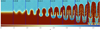 |
Fig. 7 Same as Fig. 6, but in 768 × 1536 resolution. |
| In the text | |
|
Fig. 8 ‘Hot-bubble’ experiment at time=150 and 300 s. Both panels show fluctuations of ΔA/A, with the min/max values given in the floating box. |
| In the text | |
|
Fig. 9 MHD blast experiment. Density (left) and magnetic pressure (right) at time=0.021. We note the sharp shock-fronts. |
| In the text | |
|
Fig. 10 Orszag-Tang vortex test at time = 0.5. Density (left), entropy per unit mass (middle), and magnetic pressure (right). |
| In the text | |
|
Fig. 11 Orszag-Tang vortex test at time = 0.75. Density (left), entropy per unit mass (middle), and magnetic pressure (right). We note the plasmoids forming. |
| In the text | |
|
Fig. 12 Current-sheet test at different times. Density (top) and magnetic pressure (bottom). |
| In the text | |
|
Fig. 13 Current-sheet test at different times. Density (top) and magnetic pressure (bottom). |
| In the text | |
|
Fig. 14 Magnetic-loop advection experiment. The initial magnetic pressure (left) and after the loop has been advected around the grid twice. |
| In the text | |
|
Fig. 15 Gresho vortex test. The initial setup (left) and after two rotation periods with different Mach numbers: Ma = 0.1, 0.01, 0.001. The rightmost panel is for a higher resolution run (see text for more details). |
| In the text | |
|
Fig. 16 Gas density (left) and pressure (right) in the Gresho vortex test with Ma = 0.01. We note that the quantities are within the noise limit. |
| In the text | |
|
Fig. 17 Magnetic rotor test. From left to right: Density, magnetic pressure, Mach number, and |
| In the text | |
Current usage metrics show cumulative count of Article Views (full-text article views including HTML views, PDF and ePub downloads, according to the available data) and Abstracts Views on Vision4Press platform.
Data correspond to usage on the plateform after 2015. The current usage metrics is available 48-96 hours after online publication and is updated daily on week days.
Initial download of the metrics may take a while.