| Issue |
A&A
Volume 698, May 2025
|
|
|---|---|---|
| Article Number | A288 | |
| Number of page(s) | 11 | |
| Section | The Sun and the Heliosphere | |
| DOI | https://doi.org/10.1051/0004-6361/202553839 | |
| Published online | 24 June 2025 | |
Density-gradient-driven drift-wave turbulence in the solar corona
1
Centre for Mathematical Plasma Astrophysics, KU Leuven 3001, Leuven, Belgium
2
Dutch Institute for Fundamental Energy Research, 5612 AJ Eindhoven, The Netherlands
3
Eindhoven University of Technology, 5600 MB Eindhoven, The Netherlands
4
Department of Physics & Astronomy, Ruhr-Universität Bochum, D-44780 Bochum, Germany
5
Institute of Physics, University of Maria Curie-Skłodowska, 20-031 Lublin, Poland
6
Faculty of Military Sciences, Netherlands Defence Academy, 1781 AC Den Helder, The Netherlands
⋆ Corresponding author: m.brchnelova@mindef.nl
Received:
21
January
2025
Accepted:
23
April
2025
Aims. The solar corona is a highly filamentary environment with density gradients of diverse scales and strengths. If perpendicular to the background magnetic field, such gradients give rise to drift waves (DWs) via the DW instability, leading to plasma heating and particle, heat, and momentum transport. Particularly in the context of the coronal heating and solar wind acceleration problems, it is instructive to study DWs to determine how they affect the budgets of the coronal plasma. This paper investigates density-gradient-driven DWs in the solar corona using non-linear gyrokinetic simulations, particularly fluctuation frequencies and coronal heating.
Methods. We used the gyrokinetic code GENE to simulate DW turbulence in slab geometry that represents a coronal loop. Simulations were carried out with the hydrogen mass ratio for cases with varying magnetic shear, density gradient scale lengths, and electron β, each covering ranges relevant to the corona.
Results. Frequencies between 0.1 mHz and a few hertz are obtained, with larger values possible for hotter and smaller structures. Turbulence spectra exhibit tails consistent with kinetic Alfvén wave turbulence. Particle acceleration in the parallel direction occurs, although this process only accounts for observed volumetric heating rates in regions with high gradients. In the perpendicular direction, conditions are generally such that fast stochastic heating can occur. Finally, the structure erosion timescales indicate that while DW turbulence can flatten gradients over time, most structures are expected to survive for days without additional driving.
Conclusions. Drift waves are expected to be unstable in the solar corona and can, especially when arising from strong density gradients, create an environment suitable for particle acceleration and plasma heating both parallel and perpendicular to the magnetic field on timescales of hours to days. Future modelling will assess DW behaviour in stronger gradients and in more complex configurations.
Key words: plasmas / methods: numerical / Sun: corona
© The Authors 2025
 Open Access article, published by EDP Sciences, under the terms of the Creative Commons Attribution License (https://creativecommons.org/licenses/by/4.0), which permits unrestricted use, distribution, and reproduction in any medium, provided the original work is properly cited.
This article is published in open access under the Subscribe to Open model. Subscribe to A&A to support open access publication.
1. Introduction
One of the major outstanding challenges in solar physics is solving the so-called coronal heating problem: explaining which mechanism(s) cause(s) the plasma of the solar corona to reach temperatures millions of degrees kelvin higher than the solar photosphere and chromosphere. This problem implies that one or more processes occurring on or around our closest star are poorly understood. In practice, this also means that we cannot accurately model the conditions in the solar corona, which further constrains our ability to model the solar dynamics and accurately forecast space weather. Current state-of-the-art global coronal models aimed at space weather forecasting rely on highly approximate, empirical models to add the necessary momentum and energy budgets to create a corona with realistic temperatures that drives a bi-modal solar wind (see e.g. Downs et al. 2010; Lionello et al. 2009; Baratashvili et al. 2024).
A variety of mechanisms have been proposed to explain coronal heating. An overview is provided in Klimchuk (2006). Generally, the mechanisms are divided into two classes: the processes related to magnetic reconnection and wave phenomena. Details regarding constraints on the heating due to magnetic reconnection and magnetohydrodynamic (MHD) waves can be found in the works of Aschwanden (2001) and Van Doorsselaere et al. (2020), among many others.
However, despite the substantial body of literature available on this topic, to date, there is no consensus in the community regarding the source of coronal heating. Many argue that trying to find a single process that causes coronal heating may be impossible, as it may instead be caused by several different mechanisms acting on a variety of spatial and temporal scales and interacting with each other (De Moortel & Browning 2015). Waves and instabilities can induce magnetic reconnection, and vice versa. Magnetic reconnection can lead to the formation of waves and instabilities. For example, Pueschel et al. (2014) showed that turbulence driven by magnetic reconnection on small scales gives rise to particle acceleration and a kinetic Alfvén wave (KAW) cascade, while van Ballegooijen et al. (2011) argued that Alfvénic turbulence is a strong candidate to explain coronal heating. Many phenomena observed in the solar corona, including the different types of waves and magnetic reconnection and their mutual interactions at various scales, likely contribute to the energy and momentum budgets of the coronal plasma simultaneously, albeit to a different extent.
When studying some of the possible heating processes discussed in the publications cited above, MHD and multi-fluid models may suffice. However, higher-fidelity models may be required for other processes, particularly those occurring on scales incompatible with the assumptions of the MHD and fluid models. One such process, suggested by Vranjes & Poedts (2009a,c, 2010a,b,c, 2014) as a possible mechanism through which coronal plasma could be effectively heated, are drift waves (DWs), which occur at the scale of the ion Larmor radius. As determined from thermonuclear fusion research, DWs are generated spontaneously by DW instabilities in regions where density and/or temperature gradients exist perpendicular to the background magnetic field. Many types of DWs exist, including the fusion-plasma-relevant ion- and electron-temperature-gradient-driven instabilities (Lee & Tang 1988), trapped-electron modes (Coppi & Rewoldt 1974), and microtearing modes (Hazeltine et al. 1975). The extreme ultraviolet and X-ray corona are highly filamentary and inhomogeneous, with abundant density gradients at a variety of scales (Woo 2007; Mackay et al. 2010; DeForest et al. 2018; Chitta et al. 2022; Antolin et al. 2023). Doppler measurements indicate that structures with short density-gradient scale lengths exist down to scales of 10 km (Woo 2006). Thus, in this study, we focused on density-gradient-driven DWs.
Since DWs rely solely on density gradients for their drive, it is more interesting to study them compared to mechanisms that require a specific excitation or footpoint driving (at the correct frequencies) to generate heating (see e.g. Gudiksen 2009); for DWs to be driven to instability, all that is required is a density gradient perpendicular to a sheared background magnetic field. It may be instructive to study DWs beyond the scope of coronal heating as they may be ubiquitous in the corona, just like in thermonuclear fusion plasmas. They could thus generate (drift-Alfvén) turbulence and drive secondary reconnection, which can then trigger or interfere with other coronal processes. Furthermore, since DWs produce drift motion perpendicular to the background magnetic field, their study can help us better understand and estimate cross-field transport in the corona, which is why they are studied so intensively in thermonuclear fusion research (as discussed by e.g. Voitenko & Goossens 2004).
However, unlike some of the other mechanisms mentioned above, DWs have not yet been directly identified in solar coronal observations, possibly due to the small scales of the fluctuations they excite. Drift-wave-type instabilities do, however, play an important role in other applications, such as in fusion devices, where they are the dominant source of DW turbulent transport (Terry & Diamond 1985; Rogister 1996) and have thus been widely researched in this context.
The instability mechanism generating the density-gradient-driven DWs studied in this paper is detailed in Brchnelova et al. (2024). In brief, a density perturbation ( ) to the equilibrium density profile causes a differential response from the parallel motion of ions and electrons due to their disparate masses. This results in the generation of an electrostatic potential perturbation (
 ) and thus an electric field (
 ) is generated. The resulting E×B drift then causes advection perpendicular to B and to the background density gradient (hence the term ‘drift waves’). If the response of the electrons is non-adiabatic, for example due to electron inertia, a phase difference is created between
  and
and  , and the DWs become linearly unstable.
Fluctuations produced by unstable DWs can lead to various heating mechanisms, which in turn lead to different parallel and perpendicular temperatures, as observed in the solar atmosphere. In the perpendicular direction, stochastic heating is predicted to occur (Vranjes & Poedts 2009a,c, 2010a,b,c, 2014) due to particle motion that becomes chaotic in the presence of electrostatic field fluctuations (Cerri et al. 2021). This heating has been studied both experimentally and numerically, for example in nuclear fusion experiments (McChesney et al. 1991), in the Earth's bow shock (Stasiewicz & Eliasson 2020, 2021), and in the ionosphere (Stasiewicz et al. 2000). In the ionosphere and magnetosphere, the DWs responsible for this stochastic energisation correspond to the lower hybrid drift instability between the cyclotron and lower hybrid frequencies. However, the properties of the solar corona are fairly different from those of these environments, and thus, the resulting DW frequencies can also differ significantly. Stochastic heating further requires a sufficient gradient of the electric field. Measurements of strong and dynamic electric fields in the solar atmosphere have indeed been reported (Davis 1977; Zhang & Smartt 1986), and Vranjes & Poedts (2009b) further argue that they should be omnipresent in the solar corona and sufficient to drive stochastic heating. Chandran et al. (2013) have shown that stochastic heating can explain various solar wind features, such as the temperature ratios of different plasma species. In the parallel direction, kinetic particle acceleration can take place due to a parallel electric field (E∥) and an aligned electric current (j∥; see Pueschel et al. 2014).
However, in the DW publications cited above, the properties of DWs in the solar corona have been estimated through approximate dispersion relations that rely on several simplifying assumptions and thus only allow qualitative conclusions regarding the potential of DWs for the coronal heating problem. By contrast, in Brchnelova et al. (2024), we conducted a linear gyrokinetic (Brizard & Hahm 2007) simulation study of DWs with the gyrokinetic code GENE (Jenko et al. 2000). We found that – given that linear mode signatures such as frequencies and cross-phases, especially at the lower wavenumbers that dominate turbulent spectra, tend to carry over to the non-linear system (Dannert & Jenko 2005) – DWs are expected to be unstable in the solar corona at frequencies in the range 0.1 mHz to 1 Hz, the exact frequency depending primarily on the considered length scale, temperature, and magnetic field strength
Linear simulations, however, cannot predict the amplitude of the turbulent fluctuations because saturation will occur due to the background variation. In addition, according to the quasi-linear scalings in Dannert & Jenko (2005) and Staebler et al. (2016), turbulent fluctuation amplitude spectra typically peak at much lower wavenumbers than linear growth rate spectra. We thus expanded on Brchnelova et al. (2024) by studying the non-linear system, which enabled more quantitative insights into fluctuation amplitudes, parallel and perpendicular heating, and fluctuation spectra; this in turn provides a better understanding of the effects that DWs can have on the surrounding coronal plasma.
In Sect. 2 we introduce the gyrokinetic solver GENE and the setup used for the non-linear simulations. In Sect. 3 we present analyses of non-linear simulations, including the corresponding spectral fluxes, frequency power spectra, fluctuation spectra, kinetic particle heating, stochastic timescales, and structure erosion due to particle fluxes. In Sect. 4 the findings from Sect. 3 are interpreted in the context of the solar corona. We also extrapolate on the findings to estimate the action of DWs at higher-density gradients. The limitations of the current study are discussed in Sect. 5, and our conclusions are presented in Sect. 6.
2. Gyrokinetic simulation setup
For this study we made use of the gyrokinetic Vlasov-Maxwell solver GENE (Jenko et al. 2000), which had previously been used for studies of astrophysical and space physics applications (Pueschel 2009; Pueschel et al. 2011, 2014, 2015; Told et al. 2015, 2016), in addition to many fusion applications. Gyrokinetics is a framework suitable to study kinetic processes in environments with strong guide fields. It assumes that any background magnetic field variation occurs on much larger scales than the Larmor radius and that any processes of dynamical relevance have frequencies much lower than the cyclotron frequency (∼1 to 100 kHz in the solar corona). Gyro-averaging eliminates the timescale of the Larmor motion and one velocity coordinate; as a result, gyrokinetic simulations typically exhibit speedups of several orders of magnitude when compared to fully kinetic simulations. Discussions about the validity regime of gyrokinetic simulations in astrophysical scenarios are provided in TenBarge et al. (2014), Schekochihin et al. (2009), and Howes et al. (2006). In addition, compared to gyrokinetic particle-in-cell simulations of DW turbulence, where noise can accumulate (Nevins et al. 2006), gyrokinetic Vlasov DW simulations do not suffer from this noise accumulation, even when run for long times (see, for instance, Fig. 5a of Peeters et al. 2016).
The magnetic geometry in which DWs are simulated here is a sheared slab that represents the entire length of the coronal loop or a similar gradient structure but only a small volume around a field line, with the macroscopic reference length Lz (where z is the coordinate parallel to the magnetic field) corresponding to the length of a structure such as a coronal loop. Ions and electrons, at hydrogen mass ratio, are assumed to have equal background temperatures T0, setting the reference ion sound speed cs, in a magnetic guide field B0=Bz0, defining the ion sound Larmor radius ρs. The density gradient that drives the formation of DWs exists in the x-direction, giving rise to DWs drifting in the y-direction. The corresponding wavenumber ky is normalised to 1/ρs, as is kx, corresponding to a highly anisotropic process when comparing parallel and perpendicular scales.
As in Brchnelova et al. (2024), to explore the behaviour of DWs under various coronal conditions, several parameters are varied, namely the strength of the density gradient ωn=Lz/Ln (with the density gradient scale length Ln equal for ions and electrons), electron β and magnetic shear  . The magnetic shear
  can be generally defined as
  , where Ls is the shear length, such that B=B(∇z−(x/Ls)∇y) in a slab geometry. In Brchnelova et al. (2024), we used the standard definition of
  for toroidal systems,
  with q(x) being the safety factor profile near a flux surface located at a distance r0, corresponding to q0, from the magnetic axis. The limits of
  in the simulations are based on the field-line-twist profiles of coronal loops from Aschwanden (2019).
The baseline scenario is again defined by ωn = 100,  and β = 0, with no (equal ion and electron) temperature gradient ωT = 0. For this study, assuming the corona to be collisionless is appropriate.
The gyrokinetic distribution function is treated in Fourier space in the x-direction of the density gradient and the y-direction of wave propagation. At the same time, the z-direction along the guide field is computed using finite differencing. Velocity space covers the parallel velocity v∥ and the magnetic moment μ. Domain sizes, mode, and grid-point resolutions were chosen such that doubling any setting would not substantially alter physical observables in the turbulent state. At  , the number of grid points in the x direction and z direction are thus Nx×Nz = 128 × 80, the number of grid points in v∥ and μ and Nv∥ and Nμ are 64 and 32, respectively, the converged velocity space domains in these coordinates are, respectively, Lv∥ = 3 and Lμ = 9, and the number of the resolved ky modes is Nky = 64, with the lowest finite
  . The parallel boundary condition constrains the box size Lx and depends on the shear
  as (Beer et al. 1995)

Finally, the coefficient of the fourth-order hyper-diffusion (Pueschel et al. 2010) in the x-direction is set to Dx = 0.02, and in the z-direction, the corresponding Dz = 8; both values were determined to produce converged results.
3. Properties of drift-wave turbulence
With the code setup introduced, we now discuss the physical scenarios simulated and the corresponding results. In this section we limit ourselves to a non-dimensional discussion. More specific interpretations of these results assuming coronal conditions will be presented in Sect. 4.
3.1. Simulated scenarios
The solar corona contains a wide variety of environments, and the behaviour of DWs and the associated turbulence generally depends on all physical input parameters. Thus, in addition to the baseline scenario described in Sect. 2, simulations with varying 0≤β≤3.5·10−4 (where β = 0 is referred to as the electrostatic limit),  and 50≤ωn≤250 were conducted, as listed in Table 1. Note that the upper limit of the β range was chosen to facilitate a comparison with the solar-corona reconnection study in Pueschel et al. (2014).
Physical parameter settings and perpendicular domain sizes of non-linear simulations.
All of the cases were evolved well into the quasi-stationary state of the DW turbulence (which is independent of the initial condition), where observables are time-averaged, typically for a period (measured in ion transit times) of 5−50 Lz/cs.
3.2. Fluctuation properties
In the following, observables in the form of different moments of the distribution function taken at arbitrary times during the quasi-stationary, turbulent state are visualised: the electrostatic potential, Φ, the electron number density, n, the parallel flow velocity, u∥, and the parallel and perpendicular temperatures, T∥ and T⊥. The corresponding normalisations read
Here, ρ*=ρs/Lz is the ratio of the ion sound gyroradius to the loop length.
For case 1, which uses the electrostatic limit and thus does not produce magnetic fluctuations A∥, Fig. 1 shows these fluctuations in the x-y plane, taken at the centre in the z domain along the field line. Except for Φ, these fluctuations are comparatively isotropic in x-y (recall that the z coordinate is normalised to Lz≫ρs, owing to an extreme anisotropy between the perpendicular and parallel directions), and given the small ρ*, highlight the validity of the δf approach. Typical x-y structure sizes are of the order of 1−10ρs.
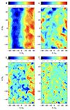 |
Fig. 1. Snapshot of fluctuation data in the quasi-stationary state for baseline case 1, with ωn = 100, |

While a proper analysis of the DW saturation mechanism is beyond the scope of this paper, the prominent zonal flow (Diamond et al. 2005) – a vertical structure in Φ at ky = 0 – in Fig. 1 suggests that zonal-flow-based energy transfer is a key process in saturating the linear instability, compare Makwana et al. (2014), Terry et al. (2021). By implication, strong zonal flows can lead to lower fluctuation amplitudes and vice versa for a given linear growth rate. Note that all cases studied, irrespective of driving gradient ωn, display similarly strong zonal flows in relation to the non-zonal (ky>0) turbulent fluctuation amplitudes. While the domain sizes Ly considered here are still on the scale of tens of gyroradii, zonal flows can in principle span much larger distances, making them a candidate for future observation efforts. Zonal flows have also been detected experimentally in fusion plasmas (Nishizawa et al. 2019), and are routinely seen in simulations of turbulence in fusion plasmas; recent work on stellarator turbulence driven by the universal instability, which is essentially the same mechanism as that studied in the present paper, reports similarly substantial amplitudes of the zonal flow (Costello et al. 2023).
For the cases with β>0, a similar zonal structure forms in the fluctuations in the magnetic vector potential A∥, as seen in Fig. 2 for case 6; given its low amplitude, however, it remains to be determined whether this feature can exert any influence on the turbulent saturation mechanism of the DWs. More importantly, however, even at low β, the appearance of magnetic fluctuations enables interactions among and between plasmoids and current sheets, allowing them to produce secondary magnetic reconnection (see Pueschel et al. 2014).
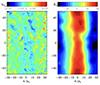 |
Fig. 2. Turbulent fluctuations for simulation case 6, where β = 10−4, allowing the system to produce magnetic perturbations A∥ (right panel). Current filaments (left panel) can thus interact via magnetic reconnection. |
3.3. Spectral fluxes
The fluctuation data shown in Figs. 1 and 2 highlight an inherent property of turbulence: the coexistence and interaction of multiple spatial scales. Typical structure sizes substantially exceed that of the fastest-growing linear mode (at ky = 4) due to mixing-length effects, allowing larger structures to substantially influence observables such as fluxes. Figure 3 shows the ky spectrum of the particle flux, normalised to n0cs(ρ*)2, for different parameter cases; the contribution of the higher wavenumbers is limited, with fluxes peaking in the range 0.1<ky<0.4. Increased  or decreased ωn, and thus reduced DW drive, shift flux peaks to slightly higher ky. The features in the heat-flux spectra are very similar, with heat fluxes (normalised to n0T0cs(ρ*)2) scaling approximately as Q∼Γ.
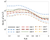 |
Fig. 3. Particle flux, Γ, as a function of ky for different parameter cases. Due to ambipolarity, electrons and ions experience equal particle fluxes. Electromagnetic contributions to the flux are negligible for all cases. |
3.4. Turbulent frequency signatures
In the absence of spectrally resolved frequency measurements, the spectral distribution of the fluctuation amplitudes – as, for instance, expressed in the fluxes – informs which frequencies are expected to be most prominent in the system overall. Power spectra for the two cases with the strongest and weakest DW drives are shown in Fig. 4. Note that in our convention, positive frequencies correspond to the drift in the ion diamagnetic direction. There, the range of frequencies widens at higher perpendicular wavenumbers, but as was seen in Fig. 3, only the lower wavenumbers, generally below ky = 0.4, are excited to large amplitudes; on small scales, energy input due to linear instabilities tends to be weak compared to non-linear transfer, resulting in highly broadened frequency signatures of low intensity. For observational purposes, the focus, therefore, lies on low-ky frequencies.
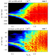 |
Fig. 4. Frequency power spectra for cases 2 (top) and 7 (bottom). Intensities are normalised separately at every ky. Narrow spectra at lower ky correspond to linear or coherent non-linear signatures, while at higher ky≳1, a strong-turbulence regime is attained. |
Linear frequencies of the dominant eigenmodes (Brchnelova et al. 2024) tend to lie in the range of −3≲ωlin≲−1 for the present parameters at wavenumbers where the non-linear frequencies are strongly coherent. However, the existence of many subdominant modes, which are substantially more difficult to probe, complicates the link between linear and non-linear physics. While future work will have to investigate this matter in more depth, at present there exists no indication that the frequency bands originating from ω≈−20 at the lowest ky and trending downwards until ky≈0.4, as well as the frequency band in the higher-shear case at positive ω for 0.3≲ky≲0.8, are corresponding to (sub-dominantly unstable) linear eigenmodes. Instead, a parallel can be drawn with heuristically similar frequency signatures (Faber et al. 2015; Pueschel et al. 2016) observed in  stellarator DW turbulence, the existence of which is not well understood.
The behaviour of the non-linear frequency ranges with changing ωn and β, however, agrees well with the linear results (with the frequencies increasing with an increasing ωn and decreasing for an increasing β). Preliminary simulations with a curved coronal loop geometry (which may be more representative of the solar corona) have revealed that with these three-dimensional effects included, the linear and non-linear frequencies are closer to each other, and they are lower than what is shown in Fig. 4, albeit only by an order-unity factor. For now, however, in this work, we are interested in an order-of-magnitude analysis, as the specific results are highly dependent on the exact values of  , β, ωn and Bz, Lz and T0, which vary significantly in the corona. Thus, while we consider the non-linear frequency ranges reported above in the subsequent analysis, one should note that more realistic dominant frequencies may be lower by a factor of a few.
3.5. Kinetic Alfvén waves
An additional observable that can be compared to in situ measurements is the turbulence spectrum. The spectral slope of the magnetic energy in the quasi-inertial range (ky≳0.7), as can be seen in Fig. 5 for case 8, is consistent with predictions in Howes et al. (2008), where KAW turbulence spectral slopes were derived for  : using the A∥ slopes measured from the present data,
  and
and  , close to the predicted −7/3. Notably, these values not only match those obtained from gyrokinetic simulations of reconnection turbulence (Pueschel et al. 2014) but are similarly consistent with observed spectra of the solar wind (Alexandrova et al. 2009; Chen et al. 2012).
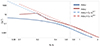 |
Fig. 5. ky (blue) and kx (red) spectra of the perturbed magnetic vector potential, A∥, along with the respective fits of |


3.6. Parallel kinetic acceleration and stochastic heating
From the perspective of solar coronal physics, a particularly interesting aspect of DWs is their ability to cause plasma heating. As discussed in the introduction, DWs may produce parallel heating via kinetic particle acceleration and perpendicular heating via triggering stochastic motion due to the electrostatic field.
To assess parallel kinetic particle acceleration, one can evaluate the DW-generated perturbed parallel electric field E∥, which enables the determination of the average volumetric heating, j∥E∥, where j∥ is the perturbed current density. This analysis was carried out for all simulation cases, with examples of the time evolution of E∥ and j∥E∥ for the baseline case 1 (electrostatic) and for case 7 (β = 3.5·10−4) shown in Fig. 6. There, E∥ is split into the static, flutter and inductive components (Pueschel et al. 2014) as
where only the first term is finite in the electrostatic limit β = 0. For the simulations with a non-zero β (allowing the generation of perturbations of the magnetic vector potential), the perturbed magnetic field projects perpendicular electric field fluctuations along the unperturbed magnetic field (see Rechester & Rosenbluth 1978), forming the flutter component, and the time variation of the perpendicular magnetic field Bx,y∼A∥ produces the inductive component. Even in the higher-β cases, however, the static component is dominant.
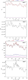 |
Fig. 6. Root-mean-square parallel electric field, E∥, normalised to |


It is important to acknowledge that the timescale over which this heating is able to alter the equilibrium distribution substantially and, thus, the background temperature is very long and ordered separately from the simulation time (t). The same applies to particle and heat fluxes, a common assumption for gyrokinetic flux-tube simulations.
The time-averaged root-mean-square j∥E∥ is listed in Table 2 in code units. The values are rounded to two significant digits due to the oscillations around the mean. As would be expected based on the linear growth rates, the volumetric heating rates most strongly scale with ωn, spanning two orders of magnitude between ω = 50 and ω = 200. Volumetric heating is also observed to decrease with  and with the electron β.
Observables from turbulence simulations.
Next, stochastic heating in the perpendicular direction is considered. Since Fig. 5 revealed that the spectrum resembles KAW turbulence, we can follow the work of Chandran (2010) on stochastic heating in Alfvén-wave (AW) turbulence. For AW and KAW fluctuations, we can express the amplitude threshold ϵi for strong stochastic heating, and from it the timescale th on which stochastic heating doubles an ion's kinetic energy, as
where v⊥i=(2kBT⊥i/mi)1/2, Ωi=qiBz/(mic), mi is the ion mass, qi the ion charge, c the speed of sound and kB the Boltzmann constant, all in cgs units. Stochastic heating is thus relevant in environments where th is sufficiently small (i.e. heating occurs on short enough timescales) to be relevant for coronal heating. For this reason, the key observable from simulations in this context is δΦ, defined here as the absolute value of the peak electrostatic fluctuation amplitude. Note that since we do not have a background electrostatic potential, δΦ=Φ. This δΦ in code units is listed in Table 2. As we have seen for the fluxes, δΦ scales strongly with ωn, resulting in stronger stochastic heating, interpreted physically later in Sect. 4 for coronal conditions.
3.7. Density structure erosion and lifetime
Finally, an essential aspect of coronal heating is the time over which this heating can be sustained – if the heating source are DWs driven by density gradients, this time is constrained by the lifetime of the density gradients. The timescale over which the gradient would erode can be estimated from the particle flux Γ (recall that due to quasi-neutrality and ambipolarity, hydrogen ions and electrons have equal number densities, equal density gradients, and equal particle fluxes) obtained from the simulations, with lifetime  , in which Ln is the density gradient scale length. For each simulated case, Γ is listed for ions in Table 2 in code units. Similarly to other observables, we see strong scaling with ωn, implying that, as expected, in the scenarios with higher density gradients, those gradients erode more quickly. Section 4 discusses these results as applied to the solar corona. As with parallel heating, we ordered out any changes to the background distributions throughout the simulation, as the simulation timescale was assumed to be much shorter than the timescale on which the structures erode. As the gradient is eroded over longer times due to the particle flux, linear DW drive will be diminished, leading to lower particle fluxes and heating rates.
In this context, however, it is helpful to recall that complete structure erosion can only occur when no restoring force exists (such a force could have been responsible for the existence of the gradient in the first place). Whether such a force persists in a given case depends on the specific scenario, and thus τΓ cannot be generalised to be relevant for all structures we see in the corona.
4. Implications for the solar corona
The results from Sect. 3 can now be interpreted physically by inserting normalisations appropriate for the solar corona. The solar corona contains various conditions and structures; however, as shown in this section, the simulated physical volumetric heating rates, timescales and frequencies, as per Sect. 3, depend heavily on the specific conditions. For this reason, we do not limit this discussion to just one set of reference parameters and instead perform evaluations for a wide range of conditions.
Since focused on the base of the corona, we considered T0 temperatures in the range 0.1 MK to 10 MK, with the smaller temperatures corresponding to, for example, prominences (Brughmans et al. 2022) and the hotter ones corresponding to super-hot coronal loops above active regions (Lu et al. 2024). Magnetic fields are taken as Bz = 0.1 G to 10 G (Alissandrakis & Gary 2021) and structure lengths Lz lie between 105 m and 108 m (Reale 2010), with the background number density determined from the electron β for β>0, or from β∼10−5 for the electrostatic cases.
4.1. Frequencies, amplitudes, and wavelengths
The magnitudes of the frequencies at the non-linearly most strongly excited wavenumbers (ky≲0.4) were in Sect. 3.4 found to vary between a few tens of cs/Lz for cases 3 and 7 up to 80 cs/Lz for case 2 (see Table 2). As cs is temperature-dependent, this quantity determines the temperature dependence of the predicted observable frequency. The results for a range of temperatures and loop lengths are shown in the top row of Fig. 7 for cases 2 and 7, with these selected as they lie on the extreme ends of the range of cases. For the set of reference coronal conditions used in Brchnelova et al. (2024), we obtain ω = 0.145 mHz and thus frequencies in the range of 0.1 to 10 mHz. Figure 7, however, reveals that hertz-range frequencies are possible for hotter and smaller structures.
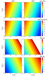 |
Fig. 7. For cases 2 (left) and 1 (right): the (absolute values of the) physical frequencies, parallel volumetric heating rates, timescales of stochastic heating, and structure lifetimes as functions of the length scale (Lz; on the x-axes) and either the background magnetic field (Bz) or the background temperature (T0). |
The obtained range agrees with the frequencies seen in the linear simulations and corresponds to the frequencies of the oscillations observed and described by Kepko et al. (2002), Kepko & Spence (2003), and Viall et al. (2009, 2021). Future study will need to reveal how DW fluctuations generated in the solar corona propagate into the solar wind, where these periodic mesoscale structures were measured. However, if these periodic structures are associated with fluctuations in the electrostatic field, they may indeed be connected to the DW mechanism.
We can also determine whether the fluctuations resolved in our simulations are directly observable in the solar corona. The strongest fluctuations were observed in case 2 and have an amplitude of a few tens of thousands. The density fluctuations are normalised to n0ρ*, meaning that if we assume B0∼10 G and Lz∼108 m, these fluctuations would correspond to ∼0.5% to 5·10−5% oscillations relative to the background density. These scale linearly with the inverse of Lz, implying that shorter structures would be more straightforwardly observable. In Fig. 1 we also see that comparable or slightly smaller relative fluctuation amplitudes are produced in T∥, T⊥ and u∥, in the case shown between 10−3% and 10−4% of the background values.
However, as evident from Figs. 1 and 2, DW oscillations occur on wavelengths of a few to a few tens of Larmor radii, which, for the investigated range of B0, corresponds to only ∼1−100 m. Resolving these scales in observations is unfeasible with current technology. Detection of DW fluctuations may become possible when DWs propagate into regions with lower magnetic fields and farther from the surface of the Sun, enabling an expansion of the associated length scales, even if DWs are no longer unstable in those regions. However, predicting the specifics of DW signatures under such circumstances is a complex task and will have to be the subject of a separate effort.
Brchnelova et al. (2024) showed that DWs have a much larger extent in the direction parallel to the background magnetic field (typically corresponding to low-order harmonics along the coronal loop). Thus, if one could conduct a measurement aligned very precisely with the magnetic field, DW fluctuations could become discernible along the coronal loop length.
4.2. Parallel and perpendicular heating
Similarly, we can quantify to what extent DWs heat the surrounding plasma in the present simulations (see Sect. 3.6). We started with parallel heating. The baseline volumetric heating rate, j∥E∥, can be obtained by applying to the value in code units the normalisation of  . Because, for a given β, the guide field
  in n0 cancels that in
  , the heating rate only depends on Lz and T0. Thus, we varied T0 and Lz across the ranges mentioned above, with the resulting j∥E∥ shown in the second row of Fig. 7.
The volumetric coronal heating that global coronal models require to heat the corona sufficiently and accelerate the solar wind is in the range of ∼10−6−10−3 erg/(cm3s), depending on the scenario considered (see e.g. Baratashvili et al. 2024). The values displayed in Fig. 7 are well below this range. However, heating increases significantly with increasing ωn. The maximum density gradient modelled in the present paper is ωn = 250 due to computational-resource limitations. However, density gradients across coronal loops of thousands or more may well be realistic (see, for instance, the discussion in Brchnelova et al. 2024 about the work of Cargill et al. 2016). We thus performed an extrapolation from the existing data to determine at which ωn parallel heating via j∥E∥ can become significant (see Sect. 4.4).
In the perpendicular direction, we evaluated whether stochastic heating can reach relevant levels based on the work of Chandran (2010) and the fluctuations of the electrostatic potential, δΦ, as outlined in Sect. 3.6. The maximum electrostatic potential fluctuations shown in our simulations range between 500 and 8·104 in code units, normalised to (T0,eV/e)ρ* (see Table 2). For example, for a 10 G field with a loop length of 108 m, we obtain voltage fluctuations between 5·10−4 V (for case 7) and 8·10−2 V (for case 2).
We then determined τh using Eq. (4). As would be expected, τh is highly sensitive to the constituents of ϵi as a result of the exponential term, and the value of ϵi is primarily dependent on B0 and Lz. For this reason, we held the plasma at 1 MK and visualise the stochastic timescale τh in the third row of Fig. 7. The exponential term quickly drives τh to very high values with increasing Lz and B0, so we only plot those regions in which τh is realistic from the perspective of coronal heating (to a maximum of a few hours). Especially for the cases with stronger density gradients, almost the entire range shown results in a substantial τh, implying that stochastic heating is very efficient in most investigated cases. As mentioned for parallel heating, these results will be extrapolated to higher density gradients in Sect. 4.4.
4.3. Erosion timescales
Finally, we quantified the lifetime, τΓ, of the gradient structures based on the particle fluxes listed in Table 2. τΓ is again most sensitive to Lz (which for a given ωn determines Ln) and to B0, affect Γ through (ρ*)2. Thus, we plot τΓ for the aforementioned ranges of Lz and B0 in the bottom row of Fig. 7. The results show that most of the structures can survive, even without continuous driving, on the timescales that correspond to the typical lifetimes of regular coronal loops (tens of minutes to hours and days; see e.g. Klimchuk et al. 2010 and Mulu-Moore et al. 2011) and longer.
4.4. Extrapolation to higher ωn
The simulations conducted here do not explore the full range of normalised density gradients expected in the corona, which may reach thousands, as discussed in Brchnelova et al. (2024). As mentioned above, simulating higher-density gradients requires numerical resolutions that exceed currently available computational resources. However, from the data listed in Table 2, we can determine extrapolation power laws that allow us to estimate ω, j∥E∥, τh (via δΦ) and τΓ (via Γi) for higher ωn. This can be determined separately for the  electrostatic and β = 3.5·10−4 sets of simulations. These are plotted in Fig. 8 along with power-law fits.
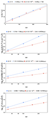 |
Fig. 8. For the electrostatic cases (blue squares) and β = 10−4 cases (red diamonds): scalings of the DW frequency (top left), parallel volumetric heating (top right), peak electrostatic potential (bottom right), and particle flux (bottom left) with the density gradient. |
Using these extrapolation laws, we estimate that at ωn = 1000, with Lz = 107 m, T0 = 1 MK and B0 = 10 G, frequencies of up to ∼700 mHz are expected, along with a relatively low parallel heating of 10−8 erg/cm3/s, a fast perpendicular stochastic heating with τh∼7·10−6 s, and long lifetimes of τΓ∼5·109 s. The drift velocity, vy, for this higher gradient would reach 1 to 10 m/s. According to the same approximations, at somewhat higher gradients ωn∼5000, the parallel heating starts to be significant (>10−5 erg/cm3/s). However, such ωn values are far above those used to create these scalings, and higher density-gradient simulations will need to be conducted in the future to confirm these findings.
However, one factor remains to be considered before concluding the efficacy of heating: the present simulations use a sheared-slab geometry, whereas a coronal loop inherently exhibits field-line curvature and even twist (Aschwanden 2019). Preliminary gyrokinetic simulations with a three-dimensional loop geometry inspired by Tsao (2023) suggest that for a given β and ωn, DW-driven turbulent amplitudes can be substantially boosted, with an order of magnitude higher Γi and two orders of magnitude higher j∥E∥ straightforwardly achievable. Further pursuit of DW turbulence in three-dimensional loop geometry will thus have a high priority going forwards, particularly as this boost makes parallel heating dynamically relevant for the solar corona at gradient scale lengths more common in this region.
5. Limitations of the modelling approach
While this work has demonstrated that DW turbulence constitutes a powerful mechanism to explain a range of observed features in the solar corona, further efforts are necessary to improve our confidence regarding the practical applications and interpretation of these results.
Firstly, this paper only considers slab geometry and does not consider curvature and twist effects. Preliminary simulations relaxing this constraint show stronger DW drive and heating.
Secondly, the present simulations technically require that magnetic field lines lie on closed flux surfaces and that fluctuations are thus (quasi-)periodic along the field line. More realistic parallel boundary conditions will need to be studied for both closed loops and regions with open field lines. It has already been suggested that line-tying of the (both background and perturbed) magnetic field does not substantially affect gyrokinetic turbulence (Tsao 2023).
Thirdly, the scenario considered here assumes no other equilibrium gradients are present. Linearly, the presence of additional temperature gradients can moderately stabilise density-gradient-driven DWs. Temperature gradients are also known to exist in the solar corona, especially in structures such as prominences, for instance, the measurements of Mouradian et al. (1979) or the models of Anzer & Heinzel (2008) and Brughmans et al. (2022). For example, from the simulations of Brughmans et al. (2022), one can estimate  in prominences, and in Brchnelova et al. (2024), we show that such ωT may have a limited influence on DW growth rates. The effect of such additional inhomogeneities could be included in future work.
6. Conclusions
We used the gyrokinetic turbulence code GENE to determine the expected properties of density-gradient-driven DW turbulence with full non-linear simulations. The geometry considered was a sheared slab representing the immediate vicinity of a magnetic field line in a coronal loop. A prescribed density gradient perpendicular to the background magnetic field leads to the spontaneous generation of DWs via the DW instability. Multiple parameter cases were computed, in which we varied the density gradient scale length, magnetic shear, and electron β to characterise the behaviour of DWs in various coronal environments. For these cases, we have the reported flux spectra, frequency power spectra, fluctuation spectra, parallel volumetric heating rates, stochastic heating timescales, and erosion timescales that indicate the possible structure lifetime without any background driving mechanism. Thereafter, for a range of background magnetic field strengths, loop lengths, and temperatures, we computed the physical values of the expected DW frequencies, parallel volumetric heating rates, stochastic heating timescales, and structure lifetimes. The main takeaways from the analysis are:
-
The self-induced DWs in the solar corona generate zonal flows, current sheets, and plasmoids, and may thus also generate an environment suitable for secondary magnetic reconnection.
-
The spectrum of the perturbed magnetic potential at the high-kx, ky tail corresponds to the slope of KAW turbulence.
-
The turbulence has a spectral peak in the range 0.1≲kyρs≲0.4, with stronger density gradients producing peaks at lower ky.
-
Depending on the loop length and temperature of the plasma, the expected DW frequencies in the solar corona range from ∼0.1 mHz to a few hertz.
-
The parallel electric fields and current densities generated by DWs may give rise to non-negligible kinetic particle acceleration in the parallel direction; simulations in more realistic geometry and/or at higher gradients will be required to confirm whether the corresponding heating rates are dynamically relevant in the solar corona.
-
The amplitude of the fluctuations of the electrostatic potential indicates that in almost all of the investigated conditions, DWs lead to fast stochastic heating in the perpendicular direction, which is consistent with the observation that T⊥>T∥ in the solar corona. Moreover, stochastic DW heating is known (from thermonuclear fusion research and experiments) to be more efficient on ions, consistent with the observation that Ti>Te in the solar corona.
-
The particle flux implies that most structures can exist despite erosion that lasts for minutes to days, even without a background driving mechanism.
-
Compared to other types of waves in the solar plasma, DWs can be distinguished by their largely electrostatic fluctuation signature.
-
However, since the wavelengths of DWs are only a few to a few tens of Larmor radii, our current instruments can only observe them if they are generated in or propagated into regions of very weak magnetic fields. Propagation of DWs from the corona into the solar wind should thus be further studied so that missions, such as the Solar Orbiter and Parker Solar Probe, can identify them.
As discussed in Sect. 5, future work will need to focus on DW turbulence in more realistic coronal loop geometry and determine the impact of realistic boundary conditions. Such studies could also include a moderate temperature gradient. In addition, the impact of possible non-thermal components of the background electron distribution should be assessed, as they may affect DW frequencies and growth rates.
Our results suggest that DWs can trigger both parallel and perpendicular heating and produce frequencies and turbulence spectra consistent with observations in the solar wind. This highlights the considerable potential of DWs in solar physics while simultaneously showing that gyrokinetic turbulence simulations can be a powerful tool even when applied to physical scenarios very different (Pueschel et al. 2017) from terrestrial plasma confinement experiments.
Acknowledgments
This research was funded by projects C16/24/010 (C1 project Internal Funds KU Leuven), G0B5823N and G002523N (FWO-Vlaanderen), and 4000145223 (SIDC Data Exploitation (SIDEX2). The resources and services used in this work were provided by the VSC (Flemish Supercomputer Centre), funded by the Research Foundation–Flanders (FWO) and the Flemish Government, and by the Tier 1 VSC grant project 2023/019. SP is also funded by the European Union. Views and opinions expressed are, however, those of the author(s) only and do not necessarily reflect those of the European Union or ERCEA. Neither the European Union nor the granting authority can be held responsible for them. His project (Open SESAME) has received funding under the Horizon Europe programme (ERC-AdG agreement No 101141362).
References
- Alexandrova, O., Saur, J., Lacombe, C., et al. 2009, Phys. Rev. Lett., 103, 165003 [NASA ADS] [CrossRef] [Google Scholar]
- Alissandrakis, C. E., & Gary, D. E. 2021, Front. Astron. Space Sci., 7, 77 [CrossRef] [Google Scholar]
- Antolin, P., Dolliou, A., Auchère, F., et al. 2023, A&A, 676, A112 [NASA ADS] [CrossRef] [EDP Sciences] [Google Scholar]
- Anzer, U., & Heinzel, P. 2008, A&A, 480, 537 [NASA ADS] [CrossRef] [EDP Sciences] [Google Scholar]
- Aschwanden, M. J. 2001, ApJ, 560, 1035 [NASA ADS] [CrossRef] [Google Scholar]
- Aschwanden, M. J. 2019, ApJ, 874, 131 [NASA ADS] [CrossRef] [Google Scholar]
- Baratashvili, T., Brchnelova, M., Linan, L., Lani, A., & Poedts, S. 2024, A&A, 690, A184 [NASA ADS] [CrossRef] [EDP Sciences] [Google Scholar]
- Beer, M. A., Cowley, S. C., & Hammett, G. W. 1995, Phys. Plasmas, 2, 2687 [Google Scholar]
- Brchnelova, M., Pueschel, M. J., & Poedts, S. 2024, Phys. Plasmas, 31, 092902 [Google Scholar]
- Brizard, A. J., & Hahm, T. S. 2007, RMP, 79, 421 [Google Scholar]
- Brughmans, N., Jenkins, J. M., & Keppens, R. 2022, A&A, 668, A47 [NASA ADS] [CrossRef] [EDP Sciences] [Google Scholar]
- Cargill, P. J., De Moortel, I., & Kiddie, G. 2016, ApJ, 823, 31 [NASA ADS] [CrossRef] [Google Scholar]
- Cerri, S. S., Arzamasskiy, L., & Kunz, M. W. 2021, ApJ, 916, 120 [NASA ADS] [CrossRef] [Google Scholar]
- Chandran, B. D. G. 2010, ApJ, 720, 548 [NASA ADS] [CrossRef] [Google Scholar]
- Chandran, B. D. G., Verscharen, D., Quataert, E., et al. 2013, ApJ, 776, 45 [NASA ADS] [CrossRef] [Google Scholar]
- Chen, C. H. K., Salem, C. S., Bonnell, J. W., Mozer, F. S., & Bale, S. D. 2012, Phys. Rev. Lett., 109, 035001 [NASA ADS] [CrossRef] [Google Scholar]
- Chitta, L. P., Peter, H., Parenti, S., et al. 2022, A&A, 667, A166 [NASA ADS] [CrossRef] [EDP Sciences] [Google Scholar]
- Coppi, B., & Rewoldt, G. 1974, Phys. Rev. Lett., 33, 1329 [Google Scholar]
- Costello, P., Proll, J. H. E., Plunk, G. G., Pueschel, M. J., & Alcusón, J. A. 2023, JPP, 89, 905890402 [Google Scholar]
- Dannert, T., & Jenko, F. 2005, Phys. Plasmas, 12, 072309 [Google Scholar]
- Davis, W. D. 1977, Sol. Phys., 54, 139 [Google Scholar]
- De Moortel, I., & Browning, P. 2015, Philos. Trans. R. Soc. Lond. Ser. A, 373, 20140269 [Google Scholar]
- DeForest, C. E., Howard, R. A., Velli, M., Viall, N., & Vourlidas, A. 2018, ApJ, 862, 18 [Google Scholar]
- Diamond, P. H., Itoh, S. I., Itoh, K., & Hahm, T. S. 2005, Plasma Phys. Control F., 47, R35 [Google Scholar]
- Downs, C., Roussev, I. I., van der Holst, B., et al. 2010, ApJ, 712, 1219 [CrossRef] [Google Scholar]
- Faber, B. J., Pueschel, M. J., Proll, J. H. E., et al. 2015, Phys., Plasmas, 22 [CrossRef] [Google Scholar]
- Gudiksen, B. V. 2009, ASR, 43, 108 [Google Scholar]
- Hazeltine, R. D., Dobrott, D., & Wang, T. S. 1975, Phys. Fluids, 18, 1778 [Google Scholar]
- Howes, G. G., Cowley, S. C., Dorland, W., et al. 2006, ApJ, 651, 590 [NASA ADS] [CrossRef] [Google Scholar]
- Howes, G. G., Dorland, W., Cowley, S. C., et al. 2008, Phys. Rev. Lett., 100, 065004 [NASA ADS] [CrossRef] [Google Scholar]
- Jenko, F., Dorland, W., Kotschenreuther, M., & Rogers, B. N. 2000, Phys. Plasmas, 7, 1904 [Google Scholar]
- Kepko, L., & Spence, H. E. 2003, J. Geophys. Res. (Space Phys.), 108, 1257 [Google Scholar]
- Kepko, L., Spence, H. E., & Singer, H. J. 2002, Geophys. Res. Lett., 29, 39 [Google Scholar]
- Klimchuk, J. A. 2006, Sol. Phys., 234, 41 [Google Scholar]
- Klimchuk, J. A., Karpen, J. T., & Antiochos, S. K. 2010, ApJ, 714, 1239 [NASA ADS] [CrossRef] [Google Scholar]
- Lee, W. W., & Tang, W. M. 1988, Phys. Fluids, 31, 612 [Google Scholar]
- Lionello, R., Linker, J. A., & Mikić, Z. 2009, ApJ, 690, 902 [CrossRef] [Google Scholar]
- Lu, Z., Chen, F., Ding, M. D., et al. 2024, Nat. Astron., 8, 706 [Google Scholar]
- Mackay, D. H., Karpen, J. T., Ballester, J. L., Schmieder, B., & Aulanier, G. 2010, Space Sci. Rev., 151, 333 [Google Scholar]
- Makwana, K. D., Terry, P. W., Pueschel, M. J., & Hatch, D. R. 2014, Phys. Rev. Lett., 112, 095002 [Google Scholar]
- McChesney, J. M., Bellan, P. M., & Stern, R. A. 1991, Phys. Fluids B: Plasma Phys., 3, 3363 [Google Scholar]
- Mouradian, Z., Martres, M. J., & Soru-Escaut, I. 1979, A&A, 79, 138 [Google Scholar]
- Mulu-Moore, F. M., Winebarger, A. R., Warren, H. P., & Aschwanden, M. J. 2011, ApJ, 733, 59 [NASA ADS] [CrossRef] [Google Scholar]
- Nevins, W. M., Candy, J., Cowley, S., et al. 2006, Phys. Plasmas, 13, 122306 [Google Scholar]
- Nishizawa, T., Almagri, A. F., Anderson, J. K., et al. 2019, Phys. Rev. Lett., 122, 105001 [Google Scholar]
- Peeters, A. G., Rath, F., Buchholz, R., et al. 2016, Phys. Plasmas, 23, 082517 [Google Scholar]
- Pueschel, M. J. 2009, Ph.D. Thesis [Google Scholar]
- Pueschel, M. J., Dannert, T., & Jenko, F. 2010, Comput. Phys. Commun., 181, 1428 [Google Scholar]
- Pueschel, M. J., Jenko, F., Told, D., & Büchner, J. 2011, Phys. Plasmas, 18, 112102 [Google Scholar]
- Pueschel, M. J., Told, D., Terry, P. W., et al. 2014, ApJS, 213, 30 [Google Scholar]
- Pueschel, M. J., Terry, P. W., Told, D., & Jenko, F. 2015, Phys. Plasmas, 22, 062105 [Google Scholar]
- Pueschel, M. J., Faber, B. J., Citrin, J., et al. 2016, Phys. Rev. Lett., 116, 085001 [Google Scholar]
- Pueschel, M. J., Rossi, G., Told, D., et al. 2017, Plasma Phys. Control F., 59, 024006 [Google Scholar]
- Reale, F. 2010, Liv. Rev. Sol. Phys., 7, 5 [Google Scholar]
- Rechester, A. B., & Rosenbluth, M. N. 1978, Phys. Rev. Lett., 40, 38 [NASA ADS] [CrossRef] [Google Scholar]
- Rogister, A. L. 1996, Fusion Technol., 29 [Google Scholar]
- Schekochihin, A. A., Cowley, S. C., Dorland, W., et al. 2009, ApJS, 182, 310 [NASA ADS] [CrossRef] [Google Scholar]
- Staebler, G. M., Candy, J., Howard, N. T., & Holland, C. 2016, Phys. Plasmas, 23, 062518 [Google Scholar]
- Stasiewicz, K., & Eliasson, B. 2020, ApJ, 904, 173 [Google Scholar]
- Stasiewicz, K., & Eliasson, B. 2021, MNRAS, 508, 1888 [Google Scholar]
- Stasiewicz, K., Lundin, R., & Marklund, G. 2000, Phys. Scr., 2000, 60 [Google Scholar]
- TenBarge, J. M., Daughton, W., Karimabadi, H., Howes, G. G., & Dorland, W. 2014, Phys. Plasmas, 21, 020708 [Google Scholar]
- Terry, P. W., & Diamond, P. H. 1985, Phys. Fluids, 28, 5 [Google Scholar]
- Terry, P. W., Li, P. -Y., Pueschel, M. J., & Whelan, G. G. 2021, Phys. Rev. Lett., 126, 025004 [Google Scholar]
- Told, D., Jenko, F., TenBarge, J. M., Howes, G. G., & Hammett, G. W. 2015, Phys. Rev. Lett., 115, 025003 [NASA ADS] [CrossRef] [Google Scholar]
- Told, D., Cookmeyer, J., Muller, F., Astfalk, P., & Jenko, F. 2016, New J. Phys., 18, 065011 [NASA ADS] [CrossRef] [Google Scholar]
- Tsao, S. -W. 2023, Ph.D. Thesis, University of Texas, Austin, USA [Google Scholar]
- van Ballegooijen, A. A., Asgari-Targhi, M., Cranmer, S. R., & DeLuca, E. E. 2011, ApJ, 736, 3 [Google Scholar]
- Van Doorsselaere, T., Srivastava, A. K., Antolin, P., et al. 2020, Space Sci. Rev., 216, 140 [Google Scholar]
- Viall, N. M., Spence, H. E., & Kasper, J. 2009, Geophys. Res. Lett., 36 [CrossRef] [Google Scholar]
- Viall, N. M., Vourlidas, A., Howard, R., et al. 2021, BAAS, 53 [Google Scholar]
- Voitenko, Y., & Goossens, M. 2004, ApJ, 605, L149 [Google Scholar]
- Vranjes, J., & Poedts, S. 2009a, EPL, 86, 39001 [Google Scholar]
- Vranjes, J., & Poedts, S. 2009b, MNRAS, 400, 2147 [Google Scholar]
- Vranjes, J., & Poedts, S. 2009c, MNRAS, 398, 918 [Google Scholar]
- Vranjes, J., & Poedts, S. 2010a, MNRAS, 408, 1835 [Google Scholar]
- Vranjes, J., & Poedts, S. 2010b, ApJ, 719, 1335 [NASA ADS] [CrossRef] [Google Scholar]
- Vranjes, J., & Poedts, S. 2010c, in New Frontiers in Advanced Plasma Physics, eds. B. Eliasson, & P. K. Shukla, AIP Conf., 1306, 201 [Google Scholar]
- Vranjes, J., & Poedts, S. 2014, J. Phys. Conf. Ser., 511, 012054 [Google Scholar]
- Woo, R. 2006, ApJ, 639, L95 [Google Scholar]
- Woo, R. 2007, Sol. Phys., 241, 251 [Google Scholar]
- Zhang, Z., & Smartt, R. N. 1986, Sol. Phys., 105, 355 [Google Scholar]
All Tables
Physical parameter settings and perpendicular domain sizes of non-linear simulations.
All Figures
|
Fig. 1. Snapshot of fluctuation data in the quasi-stationary state for baseline case 1, with ωn = 100, |
| In the text | |
|
Fig. 2. Turbulent fluctuations for simulation case 6, where β = 10−4, allowing the system to produce magnetic perturbations A∥ (right panel). Current filaments (left panel) can thus interact via magnetic reconnection. |
| In the text | |
|
Fig. 3. Particle flux, Γ, as a function of ky for different parameter cases. Due to ambipolarity, electrons and ions experience equal particle fluxes. Electromagnetic contributions to the flux are negligible for all cases. |
| In the text | |
|
Fig. 4. Frequency power spectra for cases 2 (top) and 7 (bottom). Intensities are normalised separately at every ky. Narrow spectra at lower ky correspond to linear or coherent non-linear signatures, while at higher ky≳1, a strong-turbulence regime is attained. |
| In the text | |
|
Fig. 5. ky (blue) and kx (red) spectra of the perturbed magnetic vector potential, A∥, along with the respective fits of |
| In the text | |
|
Fig. 6. Root-mean-square parallel electric field, E∥, normalised to |
| In the text | |
|
Fig. 7. For cases 2 (left) and 1 (right): the (absolute values of the) physical frequencies, parallel volumetric heating rates, timescales of stochastic heating, and structure lifetimes as functions of the length scale (Lz; on the x-axes) and either the background magnetic field (Bz) or the background temperature (T0). |
| In the text | |
|
Fig. 8. For the electrostatic cases (blue squares) and β = 10−4 cases (red diamonds): scalings of the DW frequency (top left), parallel volumetric heating (top right), peak electrostatic potential (bottom right), and particle flux (bottom left) with the density gradient. |
| In the text | |
Current usage metrics show cumulative count of Article Views (full-text article views including HTML views, PDF and ePub downloads, according to the available data) and Abstracts Views on Vision4Press platform.
Data correspond to usage on the plateform after 2015. The current usage metrics is available 48-96 hours after online publication and is updated daily on week days.
Initial download of the metrics may take a while.