| Issue |
A&A
Volume 698, June 2025
|
|
|---|---|---|
| Article Number | A50 | |
| Number of page(s) | 9 | |
| Section | The Sun and the Heliosphere | |
| DOI | https://doi.org/10.1051/0004-6361/202452312 | |
| Published online | 28 May 2025 | |
Coronal jet Identification with machine learning
1
Solar Physics and Space Plasma Research Centre (SP2RC), School of Mathematical and Physical Science, University of Sheffield, Hicks Bldg, Hounsfield Road, Sheffield S3 7RH, UK
2
Department of Physics, University of Rome “Tor Vergata”, Via della Ricerca Scientifica 1, Rome I-00133, Italy
3
Instituto de Astrofísica e Ciências do Espaço, Department of Physics, University of Coimbra, Coimbra, Portugal
4
Department of Astronomy, Eötvös Loránd University, Pázmány P. sétány 1/A, Budapest H-1117, Hungary
5
Gyula Bay Zoltan Solar Observatory (GSO), Hungarian Solar Physics Foundation (HSPF), Petőfi tér 3., Gyula H-5700, Hungary
6
National Key Laboratory of Deep Space Exploration, School of Earth and Space Sciences, University of Science and Technology of China, Hefei 230026, People’s Republic of China
7
CAS Key Laboratory of Geospace Environment, Department of Geophysics and Planetary Sciences, University of Science and Technology of China, Hefei 230026, People’s Republic of China
8
School of Electrical and Electronic Engineering, University of Sheffield, Amy Johnson Building, Portabello Street, Sheffield S1 3JD, UK
⋆ Corresponding author: This email address is being protected from spambots. You need JavaScript enabled to view it.
Received:
19
September
2024
Accepted:
5
March
2025
Abstract
Coronal jets are narrow eruptions observable across various wavelengths, primarily driven by magnetic activity. These phenomena may play a pivotal role in solar activity, which significantly impacts the dynamics of the solar system, however they have not been studied in depth thus far. This work employs machine learning, specifically, via a random forest model, to enhance the assembly of the dataset of coronal jets. By combining data from two segmentation methods, semi-automated jet identification algorithm (SAJIA) and mathematical morphology (MM), we strove to develop a more comprehensive dataset. Our model was trained and validated initially on a robust dataset and subsequently applied to classify unlabelled data. To ensure a higher level of confidence for positive identifications, the classification threshold was increased to 0.95. This adjustment led to the identification of 3452 new jet candidates. The new candidates were then validated through visual inspection. The validation resulted in the identification of 3268 true jets and 184 false positives. Our findings highlight the effectiveness of integrating machine learning with traditional analysis techniques to enhance the accuracy and reliability of solar jet identification. These results contribute to a deeper understanding of coronal jets and their role in solar dynamics, demonstrating the potential of machine learning in advancing solar physics research.
Key words: Sun: activity / Sun: filaments / prominences
© The Authors 2025
 Open Access article, published by EDP Sciences, under the terms of the Creative Commons Attribution License (https://creativecommons.org/licenses/by/4.0), which permits unrestricted use, distribution, and reproduction in any medium, provided the original work is properly cited.
This article is published in open access under the Subscribe to Open model. This email address is being protected from spambots. You need JavaScript enabled to view it. to support open access publication.
1. Introduction
Solar activity plays a crucial role in the dynamics of the solar system, both on short- and long-term timescales, especially given the impact on Earth and other celestial bodies at present. Coronal jets are narrow, elongated eruptions occurring within the Sun’s corona, observable across various wavelengths (Shibata et al. 1992; Raouafi et al. 2016; Liu et al. 2023). Similarly to major dynamic solar phenomena, including solar flares and coronal mass ejections (CMEs), most theoretical and observational studies suggest that coronal jets fundamentally originate from magnetic reconnection phenomena (Shibata et al. 1992; Canfield et al. 1996; Moore et al. 2010; Pariat et al. 2015; Sterling et al. 2015).
Nevertheless, another category of magnetohydrodynamics (MHD) models highlights a distinct mechanism for the onset of coronal jets, which is not the emergence of magnetic flux itself, but rather the injection of helicity through photospheric motions (Pariat et al. 2015, 2016; Raouafi et al. 2016). Specifically, shear and/or twisting motions at the base of the closed non-potential region below a pre-existing null-point can induce magnetic reconnection with the surrounding quasi-potential flux, thereby initiating untwisting or helical jets (see e.g. Pariat et al. 2015). Moreover, previous studies have shown that coronal jet evolution is often preceded by wave-like or oscillatory disturbances (Pucci et al. 2012; Scullion et al. 2012; Bagashvili et al. 2018). Observational analyses have revealed that many jets are associated with oscillations in coronal emission at the jet bases, which may result from changes in the area or temperature of the pre-jet activity region (Pucci et al. 2012). Statistically, pre-jet intensity oscillations have been observed around 12–15 minutes before jet onset (Bagashvili et al. 2018) and they are potentially linked to MHD wave generation, driven by rapid temperature variations and shear flows associated with local reconnection events (Shergelashvili et al. 2006).
Additionally, their chromospheric counterparts (or even so-called smaller cousins), known as spicules (length ∼10 Mm), play a crucial role in the coronal heating and the acceleration of the solar wind (De Pontieu et al. 2004; Shibata et al. 2007; Tian et al. 2014; Dey et al. 2022; Liu et al. 2023), which are yet not fully understood.
In this work, we approach the coronal jet problem from another angle considering whether there is a solar cycle effect on these localised dynamic features. Although the solar cyclic activity is marked by a series of global phenomena, such as the long-term evolution of sunspot numbers, variations in solar irradiance, and the frequency of solar flares and CMEs (Solanki & Krivova 2011; Song et al. 2016; Bhowmik & Nandy 2018), the extent and mechanisms through which the solar cycle influences localised small-scale solar features, such as coronal jets, remain poorly understood. This lack of clarity underscores the necessity for comprehensive statistical studies. Shimojo et al. (1996) studied 100 jets, predominantly originated from active regions, over the period from November 1991 to April 1992, upon manual examination of the X-ray observations from the Yohkoh Soft X-Ray Telescope (Ogawara 1995).
More recently, Liu et al. (2023) introduced a novel semi-automated identification algorithm for off-limb coronal jets: the semi-automated jet identification algorithm (SAJIA). They applied SAJIA to data collected by the Atmospheric Imaging Assembly (AIA; Lemen et al. 2012) aboard the Solar Dynamics Observatory (SDO) throughout Solar Cycle 24, spanning 2010 through 2020. The jet events analysed in this study have been identified using the SDO/AIA 304 Å channel, which primarily captures emissions from He II at temperatures around 50 000 K, with possible contributions from slightly higher temperatures, but cooler than typical coronal plasma. Although these features may not reach canonical coronal temperatures, they are spatially located within the corona and exhibit the characteristic morphology and dynamic behaviour of jet-like ejections. Additionally, previous studies have shown that many jets observed in 304 Å correspond to multi-thermal events, where cooler plasma is ejected alongside or as a consequence of coronal reconnection processes (Morton et al. 2012; Monga et al. 2021; Raouafi et al. 2016; Shen 2021; Liu et al. 2023).
Moreover, Liu et al. (2023) observed power-law distributions relating the intensity and energy to the frequency of the 1215 jets identified using SAJIA. Additionally, quasi-annual oscillations in their properties were also revealed, providing insights into the temporal dynamics of these solar phenomena.
More recent studies have leveraged machine learning to uncover cyclical patterns in solar phenomena. Diercke et al. (2024) employed a deep learning detection algorithm to identify a filament cycle based on H-alpha observations during solar cycle 24. Similarly, Zhang et al. (2024) revealed a prominence cycle within the same solar cycle by applying a deep learning approach to analyze images from SDO/AIA at 304 Å images. These advancements highlight the growing application of machine learning techniques to enhance our understanding of the cyclic nature of solar activities. Such studies can help decipher the underlying physical processes that link the broader solar cycle with the behaviour of smaller-scale phenomena like coronal jets. This deeper understanding is crucial for advancing our knowledge of solar dynamics and improving our ability to predict space weather events that have a direct impact on Earth’s technological infrastructure.
In a recent study, Bourgeois et al. (2025) leveraged SDO/AIA images to gather detailed information about solar structures during Solar Cycle 24. These authors employed mathematical morphology (MM), a technique fundamentally rooted in the analysis of geometric structures, to study both eruptive and atmospheric phenomena on the Sun. Through the application of these advanced mathematical tools, they were able to efficiently analyze and interpret the complex and dynamic features of solar phenomena. Their work not only provided comprehensive statistics on solar activity, but also delivered critical insights into active longitudes, enhancing our understanding of solar behaviour during this cycle.
In this paper, we employ a popular machine learning approach, namely, random forests, to augment the jets dataset obtained from Liu et al. (2023). Random forests is an ensemble of learning method that builds multiple decision trees during training and outputs the mode of the classes of the individual trees. This method is highly regarded for its accuracy, robustness, and ability to handle large datasets with numerous input variables.
To enhance the available dataset, we combined jet structures identified by SAJIA with those found through the application of MM, which offers valuable tools for various tasks, such as image enhancement, shape and size analysis, skeletonisation, multi-scale analysis, background subtraction, and noise removal. In solar physics, MM is primarily utilised for feature detection, segmentation, and tracking solar events, such as filament detection.
Although MM has its roots in the early 1960s (Matheron 1967; Haas et al. 1967; Serra 1969), its use in solar physics has only become prevalent in more recent times. In solar physics, MM is predominantly used for feature detection, segmentation, and tracking solar events (Shih & Kowalski 2003; Koch & Rosolowsky 2015; Barata et al. 2018; Carvalho et al. 2020; Bourgeois et al. 2024). The combination of SAJIA and MM techniques allows for a more comprehensive dataset to be constructed by leveraging the strengths of both analytical approaches, therby providing a richer basis for understanding and predicting solar jet phenomena.
The structure of the paper is as follows. Section 2 provides a detailed description of the dataset used in this study. Sections 3 and 4 outline the methodological framework and present a comprehensive analysis of the classification model’s performance, including key evaluation metrics. Finally, Sect. 5 offers an in-depth interpretation of the results and concluding remarks, providing insights to further understand the model’s effectiveness and implications.
2. Data
In this section, we outline the dataset used to train the machine learning model, providing details on the process by which it was acquired. For the classification task at hand, it is essential to utilise a dataset that distinctly encodes characteristics of both positive (true coronal jets) and negative (false coronal jets) events. This is crucial because the machine learning model needs to learn from clear examples of each category to effectively differentiate between them. The MM description of coronal off-limb structures produced by Bourgeois et al. (2025) included a variety of features that capture the unique attributes of coronal structures, such as their morphology, intensity, and spatial distribution, so as to offer a comprehensive basis for comparison and classification.
We use the dataset proposed by Liu et al. (2023) as baseline. These authors employed the SAJIA algorithm to full-disk SDO/AIA 304 Å images from 1 June 2010, to 31 May 2020 with a temporal resolution of six hours. SAJIA yielded 3800 coronal jet candidates. Of these, 1215 were confirmed as true jets by visual inspection. Subsequently Soós et al. (2024) expanded the analysis by enhancing the temporal resolution to three hours. This refinement led to the detection of an additional 4227 coronal jet candidates within the same timeframe. From these, 1489 were validated as true jets. Overall, the combined efforts resulted in a comprehensive examination of 8027 coronal jet candidates from June 1, 2010, to May 31, 2020. Ultimately, 2704 of these detections were confirmed as true jets.
In their study, Bourgeois et al. (2025) also analyzed full-disk SDO/AIA 304 Å images ranging from 2010 to 2020, but leveraged a MM approach to identify solar structures. Such an approach has allowed for a segmentation of the coronal off-limb structures observable in the full-disk images. This methodology led to the construction of an extensive dataset comprised of MM morphology features of 877843 solar structures, providing a detailed characterisation of their geometric and topological properties (refer to Bourgeois et al. 2025 for more detailed information about the dataset). We filtered the obtained structures to retain only those closest to the solar disk by calculating the distance to the nearest pixel and applying a threshold. This filtering step is implemented to reduce noise and exclude possible eruptions located too far from the solar disk, which are less likely to be coronal jets. This ensures that our analysis is focussed on the most relevant coronal jet candidates.
In our analysis, we mapped the structures identified using the MM approach with those detected by the SAJIA algorithm based on their positions on the solar disk. Specifically, we associate each SAJIA jet candidate with the radially closest MM structure. By combining SAJIA and MM datasets, we were able to obtain a MM description of the 8027 structures from Liu et al. (2023).
After the filtering, we obtained a dataset composed of 2667 validated jets (positive events) and 5028 validated as non-jets (negative events). For the sake of clarity, throughout this work the positive events will be addressed as SAJIA jets, and the negative events will be addressed as SAJIA non-jets. Figure 1 shows the comparison of an exemplary coronal jets detected by SAJIA and the MM approach.
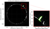 |
Fig. 1. Comparison of the contouring results from the SAJIA algorithm (red contours) and the MM algorithm (green contours) on the SDO/AIA 304 Å image recorded on 06/06/2010 at 15:00:00 UT. |
Figure 2 shows the training data obtained from the SAJIA algorithm. A key observation is that the retrieved true coronal jets tend to cluster at high absolute values of latitudes. This suggests that jets are more frequently detected at both high northern and high southern latitudes. Additionally, the number of jet detections is noticeably higher during the early stages of Solar Cycle 24. This pattern illustrates the spatial and temporal distribution of coronal jets in the training data, highlighting that certain latitudinal regions and phases of the solar cycle are more prone to jet activity. However, this is not properly representative of the natural behaviour of coronal jets. Because of the potential bias, we decided not to include latitude and time features in the input space of the model.
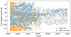 |
Fig. 2. Scatter-plot of the training data obtained from the SAJIA algorithm. Coronal jets are represented by orange dots, while non-jets are depicted in blue. |
We employed MM features to encode the descriptions of coronal jet candidates. Such features were obtained leveraging the DIPlib Python package, which provides access to various morphological metrics such as Feret diameters, radius statistics, convex area, and perimeter. Next, following a feature selection process, we eliminated collinear features to enhance model performance. This process ensures that the remaining features contribute uniquely to the classification task.
At the end of the selection process, the feature space is composed of 17 features, encoding each jet instance. The candidate jets descriptors are the total intensity, the structures area and perimeter, the length-width ratio, the skewness and excess kurtosis of the grey-value image intensities across the object, the Podczeck shape descriptors (square, circle and elongation), the measure of similarity to a circle (circularity), the roundness, the deviation from an elliptic shape (ellipse variance), the bending energy of the structure, and, finally, the position of the closest pixel to the center of the solar disk defined by the angle and the distance (for detailed information, please refer to the DIPlib documentation).
3. Methods
We employed the random forest model (Breiman 2001), an exemplary implementation of the Bootstrap aggregating (bagging) technique. Bagging is a robust ensemble learning method where each model in the ensemble operates on a slightly different subset of the training data, generated by randomly sampling the original training set with replacement. This approach ensures that each predictor within the ensemble, despite having been trained using the same algorithm, still continues to learn from a unique variations among the training data.
The random forest model combines multiple decision trees, each built from randomly sampled subsets of the data. These trees operate independently and in parallel, making predictions collaboratively. For a classification problem, the ensemble’s final prediction is typically determined by majority voting, where the class predicted by the most individual trees is chosen as the final output. This method effectively reduces the model’s variance and minimises overfitting, thereby enhancing the generalisability of the predictions. By leveraging the strength of multiple learners, the random forest model provides a more reliable and stable prediction than any single tree (Breiman 1996).
In fact, such ensemble settings enable the model to determine the probability of belonging to a class. The probability for a class is determined by the proportion of trees voting for that class. If N is the total number of trees and nc is the number voting for a class, c, the probability, P(c), is  , the decision is then dependent on a threshold (typically 0.5): if P(c)≥ threshold, the instance is classified as c. Adjusting this threshold can modify the classifier’s sensitivity and specificity. The random forest model capitalises on the strengths of decision trees and bagging to reduce overfitting by averaging multiple decision trees, thereby reducing the model variance. This allows random forests to remain robust to outliers and noise.
4. Results
To train and evaluate our random forest classifier, we divided the dataset into training and test sets with an 80-20 split. This approach ensure that the model is trained on a substantial portion of the data, while preserving a separate set for unbiased performance evaluation.
Before training the model, we conducted a hyperparameter tuning process leveraging a tree-structured parzen estimator (TPE). This is a sequential model-based optimisation method (Bergstra et al. 2011), which leverages probability density functions to guide the search towards more promising regions of the hyperparameter space. This allows TPE to efficiently explore and exploit the search space, often leading to faster convergence to optimal solutions.
We employed such method through the optimisation framework Optuna (Akiba et al. 2019). The optimal settings are evaluated by means of k-fold cross validation (Kohavi 1995). Once the model is optimised and trained, we evaluate its performance on the test set. To evaluate the classifier performance, we used multiple standard metrics and we additionally reported on the confusion matrix. The confusion matrix, shown in Table 1, includes true positives (TPs), true negatives (TNs), false positives (FPs), and false negatives (FNs), which provide detailed insights into the model’s predictions. Using multiple evaluation metrics offers a broader and more comprehensive understanding of the model’s performance. This multi-metric approach helps identify strengths and weaknesses that a single metric might overlook. The evaluation scores are given in Table 2.
Confusion matrix for random forest classifier.
Evaluation metrics for the random forest classifier.
The accuracy score is 0.76, but it measures the ratio of correctly predicted instances to the total instances and it can be misleading in unbalanced datasets where one class significantly outnumbers the other. The balanced accuracy, with a score of 0.73, addresses this by evaluating the accuracy of each class individually and then averaging the results.
The model achieved a receiver operating characteristic represented by the area under the curve (ROC-AUC) score of 0.81. This metric represents the area under the receiver operating characteristic curve, which plots the true positive rate (recall) against the false positive rate for various thresholds. This suggests that the model performs reasonably well across both classes. The high specificity indicates that the model effectively identifies negative cases, thereby minimising false positives. However, the recall and precision values reveal that there is room for improvement in correctly identifying positive cases, as it misses some positives and incorrectly labels some negatives as positives.
Figure 3 illustrates the distribution of correct and incorrect predictions across different classification thresholds. The green columns represent correct predictions (true positives and true negatives), while the red bars indicate incorrect predictions (false positives and false negatives).
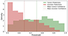 |
Fig. 3. Confidence in correct vs incorrect predictions. Distribution of correct (green) and incorrect (red) predictions across different thresholds. The x-axis represents the thresholds ranging from 0.5 to 1.0, while the y-axis indicates the count of predictions. |
The confidence of the model in correctly identifying jets also improves, as the threshold increases. In this study, our goal is to leverage machine learning to expand the sample of coronal jets. After training and validating the model, we applied it to classify previously unlabelled data. Compared to the SAJIA dataset, the MM dataset (composed of 877 843 structures) is both larger and more diverse.
To enhance the classification confidence, we increased the prediction threshold from 0.5 to 0.95, ensuring that the model only classifies an instance as a jet when it exhibits a high degree of certainty. By setting a more stringent threshold, the identified positive cases are more reliably true jets, reducing the likelihood of false positives.
The model detected 3,452 new jet candidates as a result. To further validate these findings, we performed a manual verification by visually inspecting SDO/AIA 304 Å GIF images corresponding to the eruption times of each candidate, confirming their authenticity (more details on the visual inspection process can be found in Appendix A). The visual inspection confirmed 3268 as true jets, while 184 turned out to be false positives.
Figure 5 presents an exemplary case where the new jet candidate is confirmed as a true coronal jet. Now, for the sake of clarity, let us to take a closer look at the new coronal jets identified using the MM approach. Figure 4 shows the distribution of the new detections in terms of intensity, time, latitude, and area. The figure also compares the distribution of these newly identified jet candidates (MM jets) with the jets in the training set, as well as with the non-jet instances in the training set (SAJIA jets and SAJIA non-jets, respectively), providing insights into how the newly detected events relate to the previously known samples. MM jets exhibit the highest densities at lower intensities and smaller areas, indicating that these jets are predominantly low-intensity, small-scale structures. Furthermore, MM jets are clustered primarily during the early stages of Solar Cycle 24, and are concentrated at high latitudes.
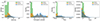 |
Fig. 4. Density distributions of MM jets, SAJIA jets, and SAJIA non-jets across four different features: intensity (A), time (B), Carrington latitude (C), and area (D). Each subplot shows the comparative density for each class, with MM jets indicated in green, SAJIA jets in orange, and SAJIA non-jets in blue. |
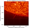 |
Fig. 5. Confirmed true jet observed on May 22, 2010. The jet is visible as a bright, elongated structure extending from the solar surface into the upper atmosphere. The image is presented in helioprojective coordinates, with the x-axis representing helioprojective longitude (Solar-X) and the y-axis representing helioprojective latitude (Solar-Y), both in arcseconds. |
In contrast, while SAJIA jets and SAJIA non-jets exhibit a more gradual decline in their frequency with increasing intensity and area, their distributions are more dispersed across latitudes and span the entire time period examined. Notably, the highest-frequency regions for SAJIA jets align closely with the clustering observed in MM jets, indicating that the newly detected MM jets follow the same spatial and temporal distribution patterns as the positive examples in the training set.
5. Conclusion
In this study, we have applied a machine learning approached based on the random forest algorithm to expand and refine the dataset of coronal jets. Our approach integrates jet structures identified by the SAJIA algorithm (Liu et al. 2023) with those detected through an MM approach (Bourgeois et al. 2025), allowing us to construct a more comprehensive and diverse dataset that enhances our understanding of coronal jet phenomena.
A key advancement in our methodology is the incorporation of MM-derived features, which provide geometric and morphological descriptors of the structures in the dataset. These additional features enrich the descriptive power of the dataset, offering a more detailed representation of coronal jets. However, while the MM dataset significantly expands the available data, it inherently lacks ground truth labels for jet classification. To address this issue, we retained the SAJIA dataset labels as the primary classification reference for training the model, ensuring a reliable and structured learning process, while leveraging the new MM features to enhance model performance.
Once it was trained and validated, the model was then applied to classify previously unlabelled data from the MM dataset. Given the absence of ground truth in this dataset, a key challenge was ensuring that new jet candidates were identified with high confidence. To achieve this aim, we adjusted the classification threshold from the default 0.5 to 0.95, meaning that the model would only assign a positive classification to jets when it reached a very high level of certainty. This more stringent criterion not only minimised the risk of false positives, but also introduced a natural consequence: the newly identified jets were predominantly clustered in the regions of the feature space where the training data exhibited the highest density of positive instances. This reflects a tendency of the model to be more conservative in its predictions, prioritising precision over recall in this application.
However, it is essential to consider the potential influence of SDO intensity degradation on the observed distributions (Ahmadzadeh et al. 2019; Barnes et al. 2020; Zwaard et al. 2021). Over time, the gradual reduction in instrument sensitivity could affect both the detection and classification of coronal jets, potentially leading to systematic biases. In particular, this degradation may have impacted the detection of small-scale, low-intensity jets, which were densely clustered between 2010 and 2012 at an approximate Carrington latitude of –75 degrees. These events, which were more prominent in the earlier period, may be underrepresented in later years due to the declining instrument sensitivity. The SAJIA algorithm, responsible for identifying jets, may have failed to detect them in subsequent periods, possibly due to an increased signal-to-noise ratio or a reduced ability to distinguish faint events from background noise.
Our approach yielded 3452 new jet candidates as a result, significantly increasing the sample size available for further analysis. To ensure the reliability of these newly identified jets, we conducted a manual validation process, which involved systematically analyzing SDO/AIA 304 Å GIF images corresponding to each candidate’s eruption time. This additional verification step confirmed 3268 true jets, while 184 were identified as false positives. These results demonstrate the robustness of our classification framework, highlighting the effectiveness of combining machine learning techniques with expert-guided validation to expand coronal jet datasets.
Beyond the immediate benefits of dataset augmentation, the expanded statistics on coronal jets allow for deeper investigations into broader solar phenomena. In particular, a more comprehensive jet catalogue may contribute to studies of active longitudes (Chidambara Aiyar 1932; Plyusnina 2010; Zhang et al. 2008; Gyenge et al. 2017), a phenomenon that remains an open question that holds far-reaching implications for solar dynamo models and space weather forecasting. However, while our results illustrate the potential of machine learning in solar physics, they also reinforce the critical importance of data quality and completeness. Machine learning models are inherently sensitive to the quality and representativeness of their training data. Thus, ensuring an accurate, well-balanced dataset remains a fundamental requirement for achieving reliable and reproducible scientific outcomes.
With the advent of new observations, particularly from Solar Orbiter’s Extreme Ultraviolet Imager (EUI), a growing number of smaller-scale jets, measuring just a few hundred kilometers in width, have been identified (Chitta et al. 2023). The identification of small-scale jets in high-resolution solar images presents new challenges for segmentation techniques. While MM has proved useful in detecting large-scale solar structures, its applicability to faint, small-scale jets (∼200–500 km wide) remains limited. The primary challenges arise from high noise levels, low contrast, and the filamentary, intermittent nature of these features, which complicate their isolation using traditional morphological operations.
However, MM could still serve as a useful pre-processing tool for enhancing jet-like structures before applying advanced segmentation methods. Techniques such as top-hat transforms, morphological gradient operators, and reconstruction-based morphological filtering could be useful in terms of contrast enhancement and edge detection. Nevertheless, more robust approaches may be necessary to accurately detect and classify small-scale jets.
Future studies could explore hybrid methodologies that integrate MM-based preprocessing with wavelet-based feature extraction and deep learning segmentation models (e.g. U-Net; Liu et al. 2024). Advanced deep learning techniques, trained on high-resolution datasets such as Solar Orbiter/EUI observations, could provide a more adaptive and automated approach to small-scale jet detection.
Advancing these detection techniques could prove insightful with respect to our understanding of the role of small-scale jets in coronal dynamics and their contribution to the solar wind. Combining MM with AI-driven feature extraction methods may pave the way for more precise and scalable segmentation strategies in solar physics, especially with the availability of new observational data.
Acknowledgments
This work is part of the SWATNet project funded by the European Union’s Horizon 2020 research and innovation programme under the Marie Skłodowska-Curie grant agreement No. 955620. We acknowledge the use of the data from the Solar Dynamics Observatory (SDO). SDO is the first mission of NASA’s Living With a Star (LWS) program. The SDO/AIA data are publicly available from NASA’s SDO website (https://sdo.gsfc.nasa.gov/data/). J.L. acknowledges the support by the National Natural Science Foundation (NSFC 12373056, 42188101) and the Strategic Priority Research Program of the Chinese Academy of Science (Grant No. XDB0560000). R.E. is grateful to Science and Technology Facilities Council (STFC, grant No. ST/M000826/1) UK, acknowledges NKFIH (OTKA, grant No. K142987 and Excellence Grant TKP2021-NKTA-64) Hungary and PIFI (China, grant number No. 2024PVA0043) for enabling this research. Sz.S. acknowledges the support (grant No. C1791784) provided by the Ministry of Culture and Innovation of Hungary of the National Research, Development and Innovation Fund (NKFIH), financed under the KDP-2021 funding scheme, furthermore the Institutional Excellence Program no. TKP2021-NKTA-64 also thank for the support received from NKFIH OTKA (Hungary, grant No. K142987). This work was also supported by the International Space Science Institute project (ISSI-BJ ID 24-604) on “Small-scale eruptions in the Sun”. MBK is grateful for the Leverhulme Trust Found ECF-2023-271 and for ÚNKP-23-4-II-ELTE-107, ELTE Hungary. S.C acknowledges the support of project CORonal mass ejection, solar eNERgetic particle and flare forecaSTing from phOtospheric sigNaturEs (CORNERSTONE), funded under the National Recovery and Resilience Plan (NRRP), Missione 4 “Istruzione e Ricerca” – Componente C2 – Investimento 1.1, “Fondo per il Programma Nazionale di Ricerca e Progetti di Rilevante Interesse Nazionale (PRIN)” – Call for tender No. 1409 of 14/09/2022 of Italian Ministry of University and Research funded by the European Union – NextGenerationEU Award Number: P2022RKXH9, Concession Decree No. 1397 of 06/09/2023 adopted by the Italian Ministry of University and Research.
References
- Ahmadzadeh, A., Kempton, D. J., & Angryk, R. A. 2019, ApJS, 243, 18 [NASA ADS] [CrossRef] [Google Scholar]
- Akiba, T., Sano, S., Yanase, T., Ohta, T., & Koyama, M. 2019, arXiv e-prints [arXiv:1907.10902] [Google Scholar]
- Bagashvili, S. R., Shergelashvili, B. M., Japaridze, D. R., et al. 2018, ApJ, 855, L21 [NASA ADS] [CrossRef] [Google Scholar]
- Barata, T., Carvalho, S., Dorotovic, I., et al. 2018, Astron. Comput., 24, 70 [NASA ADS] [CrossRef] [Google Scholar]
- Barnes, W., Cheung, M., Bobra, M., et al. 2020, J. Open Source Software, 5, 2801 [CrossRef] [Google Scholar]
- Bergstra, J., Bardenet, R., Bengio, Y., & Kégl, B. 2011, Adv. Neural Inform. Process. Syst., 24 [Google Scholar]
- Bhowmik, P., & Nandy, D. 2018, Nat. Commun., 9, 5209 [NASA ADS] [CrossRef] [Google Scholar]
- Bourgeois, S., Barata, T., Erdélyi, R., Gafeira, R., & Oliveira, O. 2024, Sol. Phys., 299 [CrossRef] [Google Scholar]
- Bourgeois, S., Chierichini, S., Soós, S., et al. 2025, A&A, 693, A301 [NASA ADS] [CrossRef] [EDP Sciences] [Google Scholar]
- Breiman, L. 1996, Mach. Learn., 24, 123 [Google Scholar]
- Breiman, L. 2001, Mach. Learn., 45, 5 [Google Scholar]
- Canfield, R. C., Reardon, K. P., Leka, K. D., et al. 1996, ApJ, 464, 1016 [NASA ADS] [CrossRef] [Google Scholar]
- Carvalho, S., Gomes, S., Barata, T., Lourenço, A., & Peixinho, N. 2020, Astron. Comput., 32, 100385 [NASA ADS] [CrossRef] [Google Scholar]
- Chidambara Aiyar, P. R. 1932, MNRAS, 93, 150 [CrossRef] [Google Scholar]
- Chitta, L. P., Zhukov, A. N., Berghmans, D., et al. 2023, Science, 381, 867 [NASA ADS] [CrossRef] [Google Scholar]
- De Pontieu, B., Erdélyi, R., & James, S. P. 2004, Nature, 430, 536 [Google Scholar]
- Dey, S., Chatterjee, P., Murthy, O. V. S. N., et al. 2022, Nat. Phys., 18, 595 [NASA ADS] [CrossRef] [Google Scholar]
- Diercke, A., Jarolim, R., Kuckein, C., et al. 2024, A&A, 686, A213 [NASA ADS] [CrossRef] [EDP Sciences] [Google Scholar]
- Gyenge, N., Singh, T., Kiss, T. S., Srivastava, A. K., & Erdélyi, R. 2017, ApJ, 838, 18 [NASA ADS] [CrossRef] [Google Scholar]
- Haas, A., Matheron, G., & Serra, J. 1967, Morphologie mathématique et granulométries en place: Annales Mines, 12, 767 [Google Scholar]
- Koch, E. W., & Rosolowsky, E. W. 2015, MNRAS, 452, 3435 [Google Scholar]
- Kohavi, R. 1995, in Proceedings of the 14th International Joint Conference on Artificial Intelligence - Volume 2, IJCAI’95 (San Francisco, CA, USA: Morgan Kaufmann Publishers Inc.), 1137 [Google Scholar]
- Lemen, J. R., Title, A. M., Akin, D. J., et al. 2012, Sol. Phys., 275, 17 [Google Scholar]
- Liu, J., Song, A., Jess, D. B., et al. 2023, ApJS, 266, 17 [NASA ADS] [CrossRef] [Google Scholar]
- Liu, J., Ji, C., Wang, Y., et al. 2024, ApJ, 972, 187 [Google Scholar]
- Matheron, G. 1967, Eléments pour une théorie des milieux poreux (Paris: Masson) [Google Scholar]
- Monga, A., Sharma, R., Liu, J., et al. 2021, MNRAS, 500, 684 [Google Scholar]
- Moore, R. L., Cirtain, J. W., Sterling, A. C., & Falconer, D. A. 2010, ApJ, 720, 757 [Google Scholar]
- Morton, R. J., Srivastava, A. K., & Erdélyi, R. 2012, A&A, 542, A70 [NASA ADS] [CrossRef] [EDP Sciences] [Google Scholar]
- Ogawara, Y. 1995, J. Atmosph. Terr. Phys., 57, 1361 [Google Scholar]
- Pariat, E., Dalmasse, K., DeVore, C. R., Antiochos, S. K., & Karpen, J. T. 2015, A&A, 573, A130 [NASA ADS] [CrossRef] [EDP Sciences] [Google Scholar]
- Pariat, E., Dalmasse, K., DeVore, C. R., Antiochos, S. K., & Karpen, J. T. 2016, A&A, 596, A36 [NASA ADS] [CrossRef] [EDP Sciences] [Google Scholar]
- Plyusnina, L. A. 2010, Sol. Phys., 261, 223 [NASA ADS] [CrossRef] [Google Scholar]
- Pucci, S., Poletto, G., Sterling, A. C., & Romoli, M. 2012, ApJ, 745, L31 [NASA ADS] [CrossRef] [Google Scholar]
- Raouafi, N. E., Patsourakos, S., Pariat, E., et al. 2016, Space Sci. Rev., 201, 1 [Google Scholar]
- Scullion, E., Rouppe van der Voort, L., & de la Cruz Rodriguez, J. 2012, in SDO-4: Dynamics and Energetics of the Coupled Solar Atmosphere. The Synergy Between State-of-the-Art Observations and Numerical Simulations, 44 [Google Scholar]
- Serra, J. 1969, Introduction à la morphologie mathématique, Cahiers du Centre de morphologie mathématique de Fontainebleau (Fontainebleau: Centre de morphologie mathématique de Fontainebleau) [Google Scholar]
- Shen, Y. 2021, Proc. R. Soc. London Ser. A, 477, 217 [NASA ADS] [Google Scholar]
- Shergelashvili, B. M., Poedts, S., & Pataraya, A. D. 2006, ApJ, 642, L73 [Google Scholar]
- Shibata, K., Ishido, Y., Acton, L. W., et al. 1992, PASJ, 44, L173 [Google Scholar]
- Shibata, K., Nakamura, T., Matsumoto, T., et al. 2007, Science, 318, 1591 [Google Scholar]
- Shih, F. Y., & Kowalski, A. J. 2003, Sol. Phys., 218, 99 [NASA ADS] [CrossRef] [Google Scholar]
- Shimojo, M., Hashimoto, S., Shibata, K., et al. 1996, PASJ, 48, 123 [Google Scholar]
- Solanki, S. K., & Krivova, N. A. 2011, Science, 334, 916 [Google Scholar]
- Song, H. Q., Zhong, Z., Chen, Y., et al. 2016, ApJS, 224, 27 [NASA ADS] [CrossRef] [Google Scholar]
- Soós, S., Liu, J., Korsós, M. B., & Erdélyi, R. 2024, ApJ, 965, 43 [CrossRef] [Google Scholar]
- Sterling, A. C., Moore, R. L., Falconer, D. A., & Adams, M. 2015, Nature, 523, 437 [NASA ADS] [CrossRef] [Google Scholar]
- Tian, H., DeLuca, E. E., Cranmer, S. R., et al. 2014, Science, 346, 1255711 [Google Scholar]
- Zhang, L. Y., Wang, H. N., & Du, Z. L. 2008, A&A, 484, 523 [NASA ADS] [CrossRef] [EDP Sciences] [Google Scholar]
- Zhang, T., Hao, Q., & Chen, P. F. 2024, ApJS, 272, 5 [NASA ADS] [CrossRef] [Google Scholar]
- Zwaard, R., Bergmann, M., Zender, J., et al. 2021, Sol. Phys., 296, 138 [NASA ADS] [CrossRef] [Google Scholar]
Appendix A: Visual inspection of coronal jets
To ensure the reliability of the automatically identified jet candidates, we conducted a systematic visual inspection of the results. Our classification approach led to the detection of 3,452 new jet candidates, each of which was subsequently verified through manual assessment. For this process, we analysed images captured by the SDO/AIA instrument at 304 Å, examining them in GIF format. The random forest model used for classification operated on single-frame representations of each event, limiting its ability to capture the temporal evolution of the detected structures. To mitigate this constraint and improve our verification process, we generated and downloaded 2 hour GIF sequences centered on the date-time of each event. This approach enabled a dynamical assessment of each candidate, allowing us to confirm whether the structures exhibited the expected morphological and kinematic behaviour characteristic of coronal jets.
In this framework, the manual validation step was crucial in distinguishing true jets from potential artifacts, false detections, or transient structures unrelated to jet activity. By incorporating human expertise into the verification process, we ensured that the identified events corresponded to real physical phenomena rather than model mis-classifications. This additional layer of validation strengthened the robustness and accuracy of the automated classification, reinforcing confidence in the final dataset of newly identified jets.
For the sake of clarity, we illustrate this process in Figure A.1, where we showcase examples of frames extracted from the GIFs used in the visual inspection. The figure presents four representative cases: FP, TP, FN, and TN.
The first row displays TP events, where the identified structures exhibit the defining characteristics of coronal jets. Each event presents a well-defined, elongated morphology extending outward from the solar surface, a hallmark of jet activity. Their brightness contrast in AIA 304 Å is distinct, with localised intensity enhancements indicative of plasma heating and ejection, features commonly associated with reconnection-driven events.
The second row presents TN events, which do not display the characteristic features of coronal jets. These structures lack the well-defined, collimated morphology typical of jets and appear more diffuse, without a clear outward extension. Their spatial and temporal behaviour further supports their classification, as they remain relatively stable over time, unlike jets, which evolve dynamically and exhibit outward propagation.
The third row illustrates FP events, where the model misclassified non-jet structures as jets. While some of these instances exhibit localised brightening, they lack the distinct, collimated morphology required for a true jet classification. Instead, they appear irregular or diffuse, with no evident plasma ejection. These features suggest that they may correspond to background brightenings, prominences, or other transient solar structures rather than actual jet events.
The fourth row presents FN events, where jets were incorrectly classified as negatives. Despite exhibiting jet-like elongation and transient behaviour, these structures may have been misclassified due to their relatively low contrast in AIA 304 Å, making them less distinguishable from the background. Some events appear more diffuse or less collimated, potentially complicating their identification. Projection effects or viewing angles may have further obscured their morphology, contributing to their misclassification.
Additionally, the model’s reliance on single-frame classification may have played a role in these false negatives. Jets that evolve gradually or exhibit weaker initial brightening might not present strong distinguishing features in an isolated frame, leading to their misclassification. This highlights a limitation of the current approach, where faint or morphologically complex jets remain challenging for the model to detect.
These examples provide insight into how different instances appear in the observational data, helping to contextualise the classification outcomes and highlighting the challenges associated with automated jet identification.
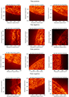 |
Fig. A.1. Illustrative examples of classification outcomes. Each row represents a classification category with three representative cases. The first row shows correctly identified coronal jets with well-defined, collimated structures and strong brightness contrast. The second row presents correctly identified non-jets, which appear diffuse and stable. The third row illustrates misclassified jets, where background features or localised brightenings were mistaken for jets. The fourth row shows missed jets, where real events were not recognised due to low contrast or projection effects. |
All Tables
All Figures
|
Fig. 1. Comparison of the contouring results from the SAJIA algorithm (red contours) and the MM algorithm (green contours) on the SDO/AIA 304 Å image recorded on 06/06/2010 at 15:00:00 UT. |
| In the text | |
|
Fig. 2. Scatter-plot of the training data obtained from the SAJIA algorithm. Coronal jets are represented by orange dots, while non-jets are depicted in blue. |
| In the text | |
|
Fig. 3. Confidence in correct vs incorrect predictions. Distribution of correct (green) and incorrect (red) predictions across different thresholds. The x-axis represents the thresholds ranging from 0.5 to 1.0, while the y-axis indicates the count of predictions. |
| In the text | |
|
Fig. 4. Density distributions of MM jets, SAJIA jets, and SAJIA non-jets across four different features: intensity (A), time (B), Carrington latitude (C), and area (D). Each subplot shows the comparative density for each class, with MM jets indicated in green, SAJIA jets in orange, and SAJIA non-jets in blue. |
| In the text | |
|
Fig. 5. Confirmed true jet observed on May 22, 2010. The jet is visible as a bright, elongated structure extending from the solar surface into the upper atmosphere. The image is presented in helioprojective coordinates, with the x-axis representing helioprojective longitude (Solar-X) and the y-axis representing helioprojective latitude (Solar-Y), both in arcseconds. |
| In the text | |
|
Fig. A.1. Illustrative examples of classification outcomes. Each row represents a classification category with three representative cases. The first row shows correctly identified coronal jets with well-defined, collimated structures and strong brightness contrast. The second row presents correctly identified non-jets, which appear diffuse and stable. The third row illustrates misclassified jets, where background features or localised brightenings were mistaken for jets. The fourth row shows missed jets, where real events were not recognised due to low contrast or projection effects. |
| In the text | |
Current usage metrics show cumulative count of Article Views (full-text article views including HTML views, PDF and ePub downloads, according to the available data) and Abstracts Views on Vision4Press platform.
Data correspond to usage on the plateform after 2015. The current usage metrics is available 48-96 hours after online publication and is updated daily on week days.
Initial download of the metrics may take a while.