| Issue |
A&A
Volume 697, May 2025
|
|
|---|---|---|
| Article Number | A191 | |
| Number of page(s) | 15 | |
| Section | Cosmology (including clusters of galaxies) | |
| DOI | https://doi.org/10.1051/0004-6361/202553940 | |
| Published online | 16 May 2025 | |
Non-halo structures and their effects on gravitationally lensed galaxies
1
Université de Strasbourg, CNRS, Observatoire Astronomique de Strasbourg (ObAS), UMR 7550, F-67000 Strasbourg, France
2
ENS Paris-Saclay, 4 Av. des Sciences, 91190 Gif-sur-Yvette, France
3
Max Planck Institute for Astrophysics, Karl-Schwarzschild-Strasse 1, D-85748 Garching bei München, Germany
4
Dipartimento di Fisica e Astronomia “Augusto Righi”, Alma Mater Studiorum Università di Bologna, Via Gobetti 93/2, I-40129 Bologna, Italy
5
INAF-Osservatorio di Astrofisica e Scienza dello Spazio di Bologna, Via Piero Gobetti 93/3, I-40129 Bologna, Italy
6
INFN-Sezione di Bologna, Viale Berti Pichat 6/2, I-40127 Bologna, Italy
7
Donostia International Physics Center (DIPC), Paseo Manuel de Lardizabal, 4, 20018 Donostia-San Sebastián, Gipuzkoa, Spain
8
Institute for Astronomy, University of Vienna, Türkenschanzstraße 17, Vienna 1180, Austria
⋆ Corresponding author: baptiste.jego@astro.unistra.fr
Received:
28
January
2025
Accepted:
31
March
2025
While the lambda cold dark matter (ΛCDM) model is very successful on large scales, its validity on smaller scales remains uncertain. Recent works suggest that non-halo dark matter structures, such as filaments and walls, could significantly influence gravitational lensing and that the importance of these effects depends on the dark matter model. Specifically, in warm dark matter (WDM) scenarios, fewer low-mass objects form and thus their mass is redistributed into the cosmic web. We investigated these effects on galaxy-galaxy lensing using fragmentation-free WDM simulations with particle masses of mχ = 1 keV and mχ = 3 keV. Although these cosmological scenarios have been observationally excluded in the past, the fraction of mass falling outside of halos grows with the thermal velocity of the dark matter particles, which allows for the search for first-order effects. We created mock datasets based on gravitationally lensed systems from the BELLS-Gallery, incorporating non-halo contributions from these simulations to study their impact in comparison to mocks where the lens has a smooth mass distribution. Using Bayesian modelling, we found that perturbations from WDM non-halo structures produce an effect on the inferred parameters of the main lens and shift the reconstructed source position. However, these variations are subtle and are effectively absorbed by standard elliptical power-law lens models, making it challenging to distinguish them from intrinsic lensing features. Most importantly, non-halo perturbations do not appear as a strong external shear term, which is commonly used in gravitational lensing analyses to represent large-scale perturbations. Our results demonstrate that while non-halo structures can affect the lensing analysis, the overall impact remains indistinguishable from variations of the main lens in colder WDM and CDM scenarios, where non-halo contributions are smaller.
Key words: gravitational lensing: strong / dark matter / large-scale structure of Universe
© The Authors 2025
 Open Access article, published by EDP Sciences, under the terms of the Creative Commons Attribution License (https://creativecommons.org/licenses/by/4.0), which permits unrestricted use, distribution, and reproduction in any medium, provided the original work is properly cited.
This article is published in open access under the Subscribe to Open model. Subscribe to A&A to support open access publication.
1. Introduction
One of the long-standing challenges and key goals of modern cosmology is to understand the nature of dark matter (see e.g. Bosma 1981; Bullock & Boylan-Kolchin 2017; Zavala & Frenk 2019). In the lambda cold dark matter (ΛCDM) paradigm, often referred to as the standard model of cosmology, dark matter particles are assumed to be non-relativistic, cold, and to make up for 85 per cent of the matter content and approximately 27 per cent of the total mass-energy budget of the Universe (see Planck Collaboration VI 2020). Generally, ΛCDM is widely used in numerical simulations, as it can accurately reproduce and predict the large-scale structure of the Universe (Frenk & White 2012); SFW. It provides a physical explanation for several crucial phenomena such as the cosmic microwave background (CMB, Planck Collaboration XVIII (2011)), the large-scale distribution of galaxies, and the accelerated expansion of the Universe.
Several models have been proposed as alternatives to CDM (see e.g. Bullock & Boylan-Kolchin 2017; Bertone & Tait 2018, for reviews) to reconcile predictions from ΛCDM with observations on galactic and sub-galactic scales. Here, we focus on models that suppress small-scale structure formation, specifically thermal relic warm dark matter (WDM) models (Bode et al. 2001). In these models, dark matter particles are produced in an equilibrium state with a non-negligible initial thermal velocity. This initial thermal velocity dispersion allows the dark matter particles to free-stream out of the gravitational potential wells of smaller perturbations, thereby suppressing the gravitational collapse of these perturbations.
Strong gravitational lensing allows us to measure the dark matter distribution on the sub-galactic scale, where the differences between models are substantial. Therefore, it provides a robust avenue for testing predictions from different dark matter models (Dalal & Kochanek 2002; Xu et al. 2009; Vegetti et al. 2018; Gilman et al. 2020; Powell et al. 2023) through the detection of low-mass dark-matter structures, where the abundance is highly sensitive to the nature of dark matter. With respect to the search for thermal relic dark matter, this approach is also complementary to other methods, such as the analysis of stellar streams (Banik et al. 2021) as well as the Lyman-α forest (Iršic et al. 2024) and Milky Way satellites (Nadler et al. 2021), with which it can be combined to produce stronger constraints (Enzi et al. 2021). However, a careful understanding of all possible sources of systematic errors is needed. For example, Richardson et al. (2022) (hereafter, R22), investigated the impact of non-halo structures on flux-ratio anomalies in multiply imaged quasars. By sampling 1000 random lines of sight, the authors show that in a mχ = 3 keV WDM scenario, neglecting the non-halo material can lead to an underestimation of the flux ratio anomalies by five to ten per cent, which increases substantially for the warmer 1 keV model. From this analysis, the authors concluded that material outside of halos, such as filaments and walls, should be included in rigorous models and that their inclusion can affect the constraints on the DM particle mass, leading to a potential bias in favour of colder dark matter models when neglected.
In this paper, we investigate whether these non-halo structures also affect the surface brightness distribution of strongly lensed arcs. The latter is sensitive to local changes of the first derivative of the lensing potential in a way that is strongly dependent on the angular resolution of the data: the better the resolution, the smaller the angular size of the perturbations that can be detected (Despali et al. 2019). Here, we aim to study the impact that non-halo structures have on lensed arc observations in different WDM scenarios. To this end, we generated and analysed a set of mock images reproducing observations of two systems studied as part of the BELLS-Gallery sample (Shu et al. 2016a; Nightingale et al. 2023; Ritondale et al. 2018). We used the new, fragmentation-free simulations from R22 to add non-halo structures to mock lensing datasets and test whether they can be detected and distinguished from the effect of the main lens. Recent studies on quadruply lensed quasars have ruled out DM models with mχ < 5.2 keV, thereby favouring colder DM particles (Hsueh et al. 2019; Gilman et al. 2020). However, these analyses neglect the effect of material outside of halos. Analyses of the WDM non-halo structures could relax these constraints. However, because these structures are extremely difficult to model, we are limited to the parameters used in R22 and their numerical requirements. As such, here we consider two models with WDM particle masses mχ = 1 and mχ = 3 keV. We note that although mχ = 1 keV has been ruled out by observations, in this work, this model serves as an interesting limiting case, allowing us to gauge the amplitude of the perturbations. The paper is structured as follows. In Sect. 2, we present the data from our WDM simulation and for the gravitational imaging. In Sect. 3, we detail the mock data that we modelled in Sect. 4. Then, in Sect. 5, we present and discuss our results. We give our conclusions in Sect. 6.
2. Simulations
2.1. Simulation parameters and models
In this work, we analyse two runs from the suite of WDM simulations presented in Stücker et al. (2022). Each volume represents a (20h−1Mpc)3 periodic box, run with cosmological WDM initial conditions generated using MUSIC1 (Hahn & Abel 2013). Both simulations were run using the same initial Gaussian random noise field and with the same cosmological parameters, h = 0.679, Ωm = 0.3051, ΩΛ = 0.6949, ΩK = 0, and σ8 = 0.8154 (Planck Collaboration VI 2020), but differ with regard to the dark matter model they represent. In particular, we used two volumes replicating cosmological structure formation in the presence of thermal relic dark matter with a particle mass of either, mχ = 1 keV or mχ = 3 keV, which we hereafter refer to as the 1 keV or 3 keV simulations, respectively.
In WDM cosmologies, the thermal velocity of DM particles leads them to have a finite free-streaming length (Bode et al. 2001), as per
which depends on the particle mass mχ, the dark matter density in units of the critical density of the Universe, Ωχ, and gχ, a dimensionless factor which accounts for the number of degrees of freedom of the dark matter particles; here, we adopt gχ = 1.5, the value corresponding to the case of sterile neutrinos.
This free-streaming motion is considered negligible in CDM, but in the case of WDM dampens the power spectrum on small scales. Here, this dampening is modelled using the Bode et al. (2001) transfer function,

where P(k) is the scale-dependant power spectrum, and k is the wavenumber vector. The resulting dampening to the power spectrum is shown in Fig. 1.
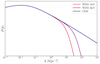 |
Fig. 1. Power spectra for CDM, mχ = 1 keV and mχ = 3 keV WDM. The WDM power spectra correspond to low-pass filtered versions of the CDM power spectrum. The vertical axis is unitless and arbitrarily normalised. The free-streaming scale is a function of the dark matter particle mass mχ, and is directly related to the cut-off scale. |
Beyond smoothing out density fluctuations, the free-streaming motion of the WDM particles allows them to escape small-scale gravitational potential fluctuations, which effectively suppresses structure formation below the half-mode mass scale,
where ρm is the mean matter density of the Universe, and
Here, Mhm corresponds to the mass at which the WDM power spectrum is suppressed by a factor of two compared to its CDM counterpart (Viel et al. 2005; Schneider et al. 2012). The WDM models used here result in a half-mode mass of Mhm = 2.5 × 10¹⁰h−1 M⊙ for the 1 keV model and Mhm = 5.7 × 10⁸h−1 M⊙ for the 3 keV model, respectively.
In general, WDM models tend to be associated with the lack of low-mass structures. While this is the main feature of these models, it is worth noting that the material that is not confined to halos remains within non-halo structures; for instance, R22 found that at z = 0, the fraction of matter outside of halos represents fnon − halo = 45.7 per cent of the total dark matter mass in the 1 keV model and, respectively, fnon − halo = 34.8 per cent in the 3 keV model. This means that in WDM models, more matter is redistributed in the smooth cosmic web large-scale structures compared to CDM, where fnon − halo is around 5%−20% and increases with redshift (e.g. Angulo & White (2010) for the 100 GeV neutralino CDM).
2.2. Avoiding artificial fragmentation
It has been found that in N-body WDM simulations, the smoother density field will artificially fragment due to discreteness effects (Wang & White 2007), resulting in a large population of spurious small mass halos. Although methods have been developed to identify and remove this spurious population (see e.g. Lovell et al. 2014; Stücker et al. 2022), these artificial halos have nevertheless prohibited the study of the smoother regions of the density fields in this type of simulation.
To circumvent this issue, another approach has been developed (Abel et al. 2012; Shandarin et al. 2012; Hahn & Abel 2013), which relies on the assumption that the DM distribution function only occupies a three dimensional hyper-surface of the full six-dimensional phase space. In these simulations, the phase0space distribution function is tessellated using a set of tracer particles, which can in turn be used to calculate the temporal evolution of the full phase space distribution function with much higher accuracy. However, these methods break down inside virialised structures due to chaotic mixing, requiring an exponentially large number of tracer particles to accurately trace these systems (Hahn & Angulo 2016; Sousbie & Colombi 2016).
The simulations used here make use of a hybrid tessellation-N-body method (Stücker et al. 2020, 2022), which dynamically separates particles into four categories: voids, walls, filaments, and halos. For the first three categories, the phase-space distribution function is tessellated using NV = 2563 particles, while the final category is modelled using NT = 5123 tracer particles of mass mT = 5.0 ⋅ 106h−1 M⊙ that are released in regions where the density field has collapsed along three dimensions (i.e. inside halos). This hybrid approach maintains the efficiency of N-body inside halos, while allowing the large-scale distribution function to be traced with very high accuracy.
An additional advantage of the hybrid tessellation-N-body approach is that it allows, in post-processing, to effectively interpolate the smooth density field down to arbitrarily small masses. This allows the creation of extremely high-resolution density maps outside of halos. It is using this property that R22 were able to project ten (8 × 8 × 8)h−3Mpc3 sub-volumes with an effective mass resolution of ∼20h−1 M⊙. Once these are put together, they represent a continuous (80 × 8 × 8)h−3Mpc3 projection. These projected density maps are shown in Fig. 2: in the upper panels, we show all the matter inside the simulation, except the halos that have been fitted and replaced by spherical NFW profiles to reduce the numerical noise; in the lower panels, we only show the matter present in non-halo structures, showing the 1 keV and 3 keV simulations in the left and right panels, respectively. As discussed previously, we can see that the 3 keV simulation contains many more low-mass halos and that the 1 keV simulation appears far smoother, with fewer visible clumps in the filaments and walls.
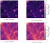 |
Fig. 2. Upper panel: Full projected data from both simulations from R22. Each square has a side length of 8h−1Mpc, and corresponds to a 80h−1 Mpc projection depth. Panel (b) contains fewer small-scale dark matter halos than panel (a) as the free-streaming length is longer in 1 keV than in 3 keV WDM. Lower panel: Non-Halo projected data from both simulations from R22. Each square has a side length of 8h−1Mpc1, and corresponds to a 80h−1Mpc1 projection. Panel (c) contains smoother and less clumpy structures at small scales than panel (d). The markers are all at the same coordinates and show the regions from which we select the non-halo material used as additional perturbations in our gravitationally lensed systems. These correspond to the highest density of non-halo material in both simulations and to the densest halo in both simulations, excluding those which are cut in the top-left corner. |
2.3. Lensing maps
From the simulated non-halo surface density maps (lower panels in Fig. 2), we compute lensing properties using the convention of Bartelmann & Schneider (2001). We define the convergence, κ, as the ratio between the surface mass density and a critical surface density, which is a function of the lens and the source angular diameters:
with c as the speed of light, G as the gravitational constant, and DL, DS, and DLS, respectively, being the angular diameter distance from the observer to the lens, the observer to the source, and from the lens to the source.
From the convergence, we can compute the lensing potential Ψ using the Poisson equation ΔxΨ(x) = 2κ. In turn, from the lensing potential we define the deflection angle maps, α1 and α2, as the individual components of the gradient, ∇xΨ(x) = α(x), along with the shear components, γ1 and γ2, as
and
where  .
.
In Fig. 3, we provide a set of example fields produced from two 20 × 20 kpc2 cut-outs of the projected density field of the same region as seen in both simulations. No direct comparison between the 3 keV and 1 keV maps can be made because the non-halo structures display different shapes and characteristics, even though they are situated at the same coordinates. Nonetheless, we observe that all the quantities have systematically higher values for 1 keV than for 3 keV, which is consistent with the higher fraction of matter outside of halos, fnon − halo, in the warmer model (see the values of fnon − halo given in Table 1).
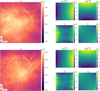 |
Fig. 3. 20 × 20 kpc2 maps of the convergence, deflection angle components, and shear components for the non-halo material in two regions around halos at the same coordinates in the 3 keV (top) and 1 keV (bottom) simulations from R22. The deflection angle maps are used to add the effect of non-halo structures on top of the deflection from the elliptical power law lenses in our datasets. The positions of the non-halo material from which we compute these convergence maps are marked in Fig. 2. They are the same in both simulations. The white contours are based on the arc light image of SDSSJ110+3649 propagated from z = 0.733. |
Parameters for the WDM cosmological simulations used in R22 and in this work.
A key parameter to consider when extracting the effect of the non-halo material from the simulations is the projection depth. Here, due to computational limitations, we only have access to data with a maximum depth of 80h−1Mpc, while typical lensed sources are located at high redshifts, resulting in observer-source distance of the order of a few gigaparsecs (Gpc). However, Σcr peaks at the typical lens redshift value for a certain source redshift, which implies that the line-of-sight perturbing material lying far away from the main lens, such as low-mass field halos, has a negligible effect on the lensed system (Despali et al. 2018). The dependence of the relative impact of the non-halo material with respect to halos on this projection depth is studied and quantified in the case of quadruply lensed quasars in R22. In that work, the authors showed that the improvements in the analysis are effectively minor when considering longer lines of sight, as their study is focussed on the relative contributions of the non-halo structures to small-mass halos. In our work, we also investigate the relative contributions of non-halo structures to unperturbed lens models. Therefore, because we have the same computational limitations as R22 and we are not looking at absolute effects, we chose to make use of the full 80h−1Mpc depth. This depth is enough to quantify the impact of the non-halo structures while avoiding having to repeat the same structures too many times; thus, we used the same projection size as in R22.
3. Mock data
We created mock lensing observations based on two strong gravitational lens systems from the eBOSS Emission-Line Lens Survey for GALaxy-Lyα EmitteR sYstems (BELLS GALLERY; Shu et al. 2016b): SDSSJ1110+3649 and SDSSJ1201+4743. We chose these specific systems because they have been studied in detail in previous works and have a reasonably good signal-to-noise ratio (S/N) level (Despali et al. 2019). They were observed with the WFC3-UVIS camera and the F606W filter on the Hubble Space Telescope. These systems have also been independently modelled by Shu et al. (2016a), Nightingale et al. (2023), and Ritondale et al. (2018). We use the lens model parameters from the latter study. Observational details on the base systems are given in Table 2. Technical details are also provided in this table, where the Einstein radii come from Ritondale et al. (2019). We created mock observations that reproduce the original HST observations in terms of resolution and noise by convolving the obtained map with an HST-type point-spread function (PSF) and adding a random noise field. We generated the noise field by independently sampling a normal random variate with a standard deviation that is ten times lower than the maximum brightness of the image to obtain a signal-to-noise ratio,  ; this result is in agreement with the typical uncertainties on the grade-A lenses magnitudes from the BELLS-Gallery (Shu et al. 2016a). The noise maps for the unperturbed and perturbed maps of the same system were computed independently. These two systems are presented in Fig. 4 with the respective image and source.
Summary of the image acquisition characteristics, and source and lens redshifts of both gravitationally lensed systems studied in this work.
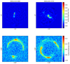 |
Fig. 4. Left panels: System SDSS J1110+3649. Right panels: System SDSS J1201+4743. The top panels represent the source brightness distribution and the bottom panels represent the observed flux after propagating through the lens, convolving with an HST-type point spread function, and adding a Gaussian noise resulting in a signal to noise ratio of 10. |
From these systems, we created three datasets: 𝒟1 and 𝒟2 based on SDSSJ1110+3649, and 𝒟3 based on SDSSJ1201+4743. Each dataset contains three variations:
-
A mock image created from the lens parameters and mock source with no additional perturbation (‘unperturbed’);
-
A mock image where perturbations in the lens plane from simulated 1 keV WDM filaments and walls (‘1 keV’) are added to the smooth case;
-
An image with perturbations in the lens plane from simulated 3 keV WDM filaments and walls (‘3 keV’).
We included the WDM perturbations to the deflection angles through the convergence maps described in the previous section. These were computed from a subregion of the full projected non-halo density maps. This subregion (marked by the white cross in Fig. 2) was chosen because it has the highest density and thus maximises the perturbative effect of the non-halo structures. Although this does not allow for a statistical study, we performed a quantitative estimation of the effect of the non-halo structures and made sure that our conclusions are not affected by the specific geometry or alignment effects in the chosen regions. This is explained in more detail in Sect. 5.
For both systems, we modelled the main deflectors using the elliptical power-law lens parameters from Ritondale et al. (2019). We added the lensing effect computed from the non-halo structure density fields to these elliptical smooth lenses. It is through the sum of these two deflectors (the main lens and non-halo perturbations) that we were able to propagate the source surface brightness distribution to produce the mock observed flux distribution. The perturbations from the simulated non-halo 1 keV and 3 keV dark matter structures (shown in the left column of Fig. 3) are the same for 𝒟1 and 𝒟3, but have been rotated by 90 degrees for 𝒟2 to check that our results are not biased by a particular alignment or anti-alignment of the filaments or walls with the intrinsic geometries of the lens mass model. Similarly, 𝒟3 was used to check that the results obtained with 𝒟1 are representative of typical gravitational lensing systems rather than outliers.
4. Lens modelling
To quantify the effect of non-halo structures, we modelled the mock data sets described above using the PRONTO code (Vegetti et al. in prep.), a grid-based Bayesian modelling technique developed by Vegetti & Koopmans (2009) and further extended by Rizzo et al. (2018), Ritondale et al. (2019), Powell et al. (2020), and Ndiritu et al. (2024). We simultaneously inferred the most probable parameters of the lens mass density distribution, ηm, along with the brightness distribution and smoothness of the background source. While the latter was modelled pixel-by-pixel in a regularised way, the former was modelled using an elliptical power-law profile (Bourassa & Kantowski 1975; Bray 1984; Kormann et al. 1994) given by
where κ0 is the surface mass density normalisation, q is the axis ratio, γ is the radial slope of the mass-density profile, and rc is the core radius, which is not a free parameter and is kept at 10−4 arcseconds. Two additional parameters account for external shear: the shear strength Γ and the shear angle, Γθ. Finally, multi-poles can be added as an extension to the elliptical power law + external shear profile. Multipoles of an order of m create a convergence, κm, which takes the form:
![$$ \begin{aligned} \kappa _{m}(r,\phi ) = r^{1-\gamma }[a_{m}\sin (m\phi ) + b_{m}\cos (m\phi )], \end{aligned} $$](/articles/aa/full_html/2025/05/aa53940-25/aa53940-25-eq11.gif)
where r and ϕ are the polar coordinates in the reference frame of the lens. These multi-poles introduce asymmetries in the lens geometry and we can measure their ability to absorb the perturbations due to external mass components (O’Riordan & Vegetti 2024; Powell et al. 2022). Here, we use multi-poles of the 3rd order or of third and fourth orders. Therefore, the most extensive form of the free parameter vector is ηm = (κ0, q, γ, xc, yc, θ, Γ, Γθ, a3, b3, a4, b4) with xc, yc, and θ the coordinates of the centre and the orientation of the lens. The values of the fiducial parameters used to create the mock data and the prior probability distributions are given in Table 3.
Values of the lens mass distribution fiducial parameters used to create the mock data and prior probability distributions to model it for 𝒟1, 𝒟2, and 𝒟3.
We explored the parameter space with the nested sampling algorithm MultiNest (Feroz et al. 2009). To compare two different models of the same dataset, we look to the logarithmic value of the evidence, log(ℰ). A lower value of log(ℰ) corresponds to a better fit of the model to the data; therefore the difference, Δlog(ℰ) = log(ℰ) – Δ0, where Δ0 is a reference value, is a quantitative way to compare the different models used for our systems. We considered four variations of the lens mass model:
-
Elliptical power law with free external shear used as a reference;
-
Elliptical power law with the external shear fixed to the best value from the previous case;
-
Elliptical power law with third-order multi-poles;
-
Elliptical power law with third- and fourth-order multi-poles.
We modelled each variation of the dataset 𝒟1 (unperturbed, 1 keV, 3 keV) with each of these. In Table 3, the priors are provided for all parameters. When a parameter was not included in the model, it was fixed at the fiducial value used to create the mock data. In the following, we focus on this system as it is the most affected by the non-halo density perturbations. A complementary discussion, including the distributions for xc, yc, and λs and the results for all three systems belonging to 𝒟1 is given in Appendix A. In the case of 𝒟2 and 𝒟3, we only fit the simple power law+external shear model to understand possible biases in 𝒟1.
Values of the differences in logarithmic evidence from the nested sampling of the parameters of each model of lens mass distribution for 𝒟1.
5. Results
In this section, we discuss the results of the lens modelling of mock images created with and without the inclusion of non-halo structures, as described in Sect. 4. For each dataset, we compared the evidence obtained by using the different mass models described in the previous section. The values of the difference in logarithmic evidence for each model are given in Table 4.
In this controlled experiment, we manually included the perturbations, as opposed to real observations, where we do not have any information on the underlying mass distribution of and around the main lens. We treated all the mock images as real observations and model them without imposing strong priors on the lens parameters. In this way, we sought to test whether it is possible to distinguish the effect of the non-halo structures from that of the main lens. In particular, we could expect their effect to appear as (or increase) the external shear, as this term is expected to represent the effect of the environment around the lens. In fact, Etherington et al. (2023) showed that the external shear term compensates for the lack of model complexity, rather than describing sources of large-scale shear. Our mocks allow us to test this hypothesis in a controlled setting.
5.1. Considering whether non-halo perturbations can be detected as external shear
In Fig. 3, we see that the shear amplitudes γ1 and γ1 are of the order of 10−3, which is similar to the range of values of external shear Γ recovered from BELLS and SLACS lenses in Ritondale et al. (2019) and Etherington et al. (2023). Therefore, we expect the effect of non-halo structures to be comparable with that of external shear. To examine this possibility, we began by modelling the mock observations of the 𝒟1 set with the simplest lens model, which includes only a power-law profile and external shear. In all cases, this simple model can fit the data quite well, leaving no persistent structures in the residuals, which have mean and median values close to zero even in the presence of the non-halo convergence. Figure 5 shows the three mocks (first column) and the results of the lens modelling. The corresponding posterior distributions are shown in Fig. 6. If external shear describes the effect of large-scale structures, we would expect an increase (or variation) of the shear parameters in the perturbed case. Instead, we see that all lens parameters are affected; in particular, the convergence normalisation, κ0, ellipticity, q, and density slope, γ. The posterior distribution for the shear strength, Γ, and angle, Γθ, do not show any systematic difference compared to the unperturbed case, suggesting that the orientation of the filaments and walls does not leave a distinctive imprint.
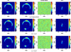 |
Fig. 5. Optimisation results when modelling the three systems from 𝒟1 with an elliptical power law + external shear. The upper panel (a) shows the results for the unperturbed system, the middle panel (b) for 1 keV, and the lower panel (c) for 3 keV. From left to right: images are the initial data, reconstructed model, normalised residuals between these two images, and reconstructed source. The units are arbitrary, but analogous to a 2D mass density |
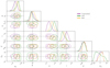 |
Fig. 6. 1σ and 2σ contours for the parameters ηm (excluding the center coordinates xc and yc, and the source regularisation λs) for the elliptical power law + external shear model of the unperturbed, 1 keV and 3 keV systems in 𝒟1. The dashed lines show the 2D distributions, the solid lines show the marginal distributions and the dotted grey lines mark the true values. |
Overall, the changes in the posterior distribution of the parameters are not significant and the best-fit values for all parameters remain sensibly the same within the 1σ error bars. The perturbations, no matter their orientations along the line of sight, seem to be reabsorbed by a reasonably smooth (unperturbed) model in both the 1 keV and 3 keV cases. Some of the differences in the mass model are absorbed by the source: as the source is pixelated and reconstructed at the same time as the lens model, the two are related and the sources react to changes in the lens model. The sources in the right column of Fig. 5 generally show the same shape and visually look similar and in very good agreement with the modelling from Ritondale et al. (2019). However, Fig. 7 shows that the differences between the resulting fine geometrical features and the source position shift lead to surface brightness differences up to half the maximum surface brightness of the source obtained for the unperturbed system. As a check that the introduction of WDM perturbations does indeed shift the sources and does not alter the overall flux, we computed the ratio of integrated surface brightness,  and
and  , where the sums are performed over all the map pixels; respectively, they yield 0.97 and 0.98. Previous works (Brainerd 2001; Koopmans 2005; Rau et al. 2013) have shown that small variations in the source structure can absorb the perturbations due to low-mass perturbations and thus prevent their detection. In this case, we see that the source can also absorb part of the effect of the extended convergence caused by the non-halo large-scale structures given that it does not visibly alter the surface brightness of the arc in a localised way.
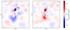 |
Fig. 7. Difference in the sources brightness distribution in the source plane obtained when modelling the systems in 𝒟1 with a lens following an elliptical power law profile with additional external shear. If SX is the source surface brightness distribution obtained for the system X, these images are the result of SUnperturbed − S1 keV (left) and SUnperturbed − S3 keV (right). The local surface brightness of the reconstructed source can be shifted and modified in the perturbed models if some of the additional perturbations are absorbed by variations of the main lens properties. The general trend given by these images is that the main effect of the additional perturbation is an overall shift of the source, which is indicated by corresponding red and blue regions of the 2D brightness distribution. To highlight this effect, the black markers give the point of highest surface brightness (‘+’ for the unperturbed system and ‘x’ for the perturbed one). |
We go on to model 𝒟2 and 𝒟3 to check if we get consistent results with the 𝒟1 analysis. Figures 8 and 9 show the corresponding posterior distributions for these two datasets. We recall here that 𝒟2 is generated from the same base system as 𝒟1, but with perturbations rotated by +90°. This is a good sanity check that our results for 𝒟1 do not emerge for specific alignments between the perturbations and other lens or source features. Comparing Figs. 6 and 8 gives us insights into the potential alignments between the source and the lens.
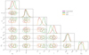 |
Fig. 8. 1σ and 2σ contours for the parameters ηm for the elliptical power law + external shear model of the unperturbed, 1 keV, and 3 keV systems in 𝒟2. The layout is the same as in Fig. 6. |
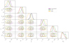 |
Fig. 9. 1σ and 2σ contours for the parameters ηm for the elliptical power law + external shear model of the unperturbed, 1 keV, and 3 keV systems in 𝒟3. The layout is the same as in Fig. 6. |
In Fig. 8, we observe that the recovered parameters lie in the same ranges as Fig. 6, where in both cases, we observe significant overlap between the posteriors corresponding to the unperturbed and perturbed lenses. This is a good qualitative indication that no parameter is strongly affected by the orientation of the perturbation. However, we can appreciate some small differences: for 𝒟2, the parameters remain the same between the unperturbed and the 3 keV systems and vary only when introducing the 1 keV perturbations, which are stronger. In 𝒟1, we instead see a gradual shift of the posterior distribution for κ0, q and γ when perturbations are introduced. Given that the perturbation orientation is the only difference between the two cases, this indicates that in 𝒟2 the alignment with the lens can conspire to mask their effect (reabsorbing it into the model even more) in the 3 keV case, as hinted by the convergence map in Fig. 3.
In 𝒟3 (Fig. 9), both the lens model and the input source are different. We nonetheless observe that the non-halo structures have a similar impact on the posteriors than that already discussed for 𝒟1 and 𝒟2. This confirms that different perturbations alter the lenses, but that they remain in statistically good agreement with each other as all the 1σ contours overlap.
5.2. Effect of lens model complexity
In the previous section, we show that an elliptical power-law+external shear parametrisation provides a good model to reconstruct the mock observations. In this section, we explore how non-halo structures affect more complex models and if this increased complexity can better capture these perturbations. As such, we analysed each mock observation within the 𝒟1 dataset with four different mass models and can compare the resulting Δlog(ℰ) values displayed in Table 4. As a first test, we fixed the external shear parameters to the best fit of the power-law + shear model. This reduced the number of parameters but decreases the quality of the lens modelling. The discrepancy between the evidence values gets bigger with the addition of non-halo perturbations, as Γ (even when it is consistent with 0 at the 1σ level) can absorb some of these perturbation effects. We note that when Γ is consistent with 0, the posterior distribution for the parameter Γθ does not converge as one cannot assign a meaningful direction to the sheer in this case (see Figs. 6, 8, 9, 10, A.1, A.2, and A.3).
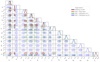 |
Fig. 10. 1σ and 2σ contours for the parameters ηm with third and fourth order multi-poles (excluding the center coordinates xc and yc, and the source regularisation λs) for the four models of the 1 keV system in 𝒟1. The reference lens model is the elliptical power law+external shear. |
We then considered a mass model with additional complexity given by third- and fourth-order multi-poles. While the input mass model used to create the mock image does not explicitly contain these multi-poles, we may expect that they may be able to capture additional features originating from the non-halo convergence. However, we find that this is not the case as for all three datasets (unperturbed, 1 keV, 3 keV), where the addition of multi-poles (m = 3 or m = 3,4) to the model decreases the evidence. Indeed, we observe that the blue and green distributions of Fig. 10 shift away from the black and red ones, corresponding more to the input source; also, they are broader and, hence, they give less precise constraints on the values of the parameters. Overall, the models with multi-poles are less preferred and the posterior distributions of the parameters are less constraining and do not help capture the effect of the perturbations. Nonetheless, it is important to note that all multi-pole parameters are consistent with 0 at the 1σ level. Looking at the differences between the values of Δlog(ℰ) for all three systems, it could be tempting to assume that since they are lower in the 1 keV scenario, multi-poles are better at absorbing 1 keV non-halo features than their 3 keV counterparts. However, we should not compare these three systems with each other and we recall that the perturbation introduced with the 1 keV and 3 keV simulations display different geometrical features.
Furthermore, looking at the distributions in Fig. 10, we can notice several similarities and differences between our four models for the 1 keV system (that are similar for the unperturbed and 3 keV systems). Most parameters follow similar posterior distributions in different models within 1σ. For all the systems, it appears that every parameter’s posterior distribution converges. The Bayesian modelling used here (Vegetti & Koopmans 2009) can provide optimised values for the lens profile in the four different types of models tested and the presence of the perturbations is marked by minor shifts in the posterior distributions of the parameters. Thus, the perturbations introduced in the strong lensing signal by WDM non-halo structures appear to be a systematic effect and they are not equivalent to multi-poles.
6. Conclusions
In this study, we have investigated whether and to what extent the material outside of halos (i.e. within the filaments and walls) can cause statistically relevant and observable effects on gravitationally lensed arcs in the case of galaxy-galaxy lensing. Such effects could be used to constrain the dark matter particle mass or, equivalently, its warmth. Here, we tested the effects of non-halo material from two simulations of WDM cosmological scenarios with dark matter particle masses, mχ = 1 keV and mχ = 3 keV. So far, most studies have focussed on the effects of dark matter halos on gravitationally lensed systems, but a recent study Richardson et al. (2022), R22 in this work) has shown that non-halo structures have an effect on quadruply lensed quasar flux ratio observations. Despite numerous simplifications, the authors show that in a mχ = 3 keV scenario, neglecting the non-halo material can lead to an underestimation of the flux ratios by 5 to 10 per cent, while this goes up to 50 per cent for mχ = 1 keV. Although this dark matter model has already been observationally ruled out, the authors concluded that non-halo material should be included in rigorous models and that their inclusion can lower the constraints on the dark matter particle mass, allowing for more permissive studies of cosmologies.
Here, we used the same WDM hybrid sheet and release simulations with mχ = 3 keV and mχ = 1 keV as in R22. These are novel fragmentation-free simulations, where particles are separated into four classes: voids, pancakes, filaments, and halos. Three of these classes (voids, pancakes, and filaments) have been simulated using 2563 sheet tracing particles, while the fourth class, halos, have been simulated using 5123N-Body particles. The sheet interpolation scheme used for the first three classes allows for the resampling of the density field in these regions with an unprecedented mass resolution. From the simulated density fields, we obtained non-halo structure convergence maps that we added as perturbations to two gravitationally lensed systems from the BELLS-Gallery. We analysed the resulting mock observations using four different models for the lens mass distribution of the systems in the first dataset and with only one of these models in the second and third datasets. Classic lens models describe the main lens with a single elliptical power law (with or without additional multi-poles), while the contribution of matter on larger scales is represented by an external shear term. Our simulated observations allowed us to test whether or not this term actually corresponds to extended mass components, such as filaments and walls, and (if so) whether they can be distinguished from the main lens model. Our main conclusions are as follows:
-
Of all the models we tested, we find that a single elliptical power-law deflector with additional external shear provides the best fit. Removing external shear or adding multi-poles does not help to account for the potential effects of non-halo structures. In fact, all the multi-pole parameters are consistent with 0 at the 1σ level.
-
When jointly reconstructing the lens and source, WDM perturbations are absorbed by the model parameters, but they do introduce a systematic bias into both the source surface brightness distribution and the lens mass-density distribution. The main effect on the reconstructed source is small localised displacements with no apparent global modulation of the shape and surface brightness.
-
We find that the commonly used singular elliptical power-law lens+external shear parametrisation is sufficient to account for most of the effect at the cost that these perturbers cannot be distinguished from others that are also absorbed by this parametrisation (Despali et al. 2021).
We conclude that in the case of galaxy-galaxy lensing, the effects of filaments and walls (i.e. the material outside of halos) can impact the reconstruction of the source surface brightness in a non-trivial way when using common lens mass profiles. However, this effect remains negligible in WDM cosmologies with mχ = 1 keV and mχ = 3 keV. Therefore, we find this applies to colder cosmologies as well, where the relative importance of non-halos compared to the one of halos is lower.
The simulated WDM non-halo material studied in this work originates from the same simulations as those used in R22; thus, we have to take the same precautions as them when interpreting our results. Our limitations are also of a similar nature: we used the thin-lens approximation, while baryonic effects were not modelled, the dark matter particles of such warmth are already observationally excluded, and the line of sight is relatively short (80h−1Mpc), compared to the sizes of typical gravitationally lensed systems. Thus, it is not possible to thoroughly quantify the effect of the non-halo structures of the line of sight and we have only considered their relative effects in the region of the main lens. Placing all non-halo structures in the lens plane maximises their effect because lensing strength scales with convergence, which is highest at that redshift. In reality, mass distributed along the line of sight contributes less due to geometric dilution and shear cancellations. Additionally, multi-plane deflections introduce non-linearities that tend to weaken the perturbations compared to a single-plane approximation. Thus, our approach provides an upper bound on the effect – if it is small here, it would be even smaller in a full ray-tracing treatment.
It is interesting to note the apparent mismatch between the conclusions of this work and those of R22. Indeed, in R22, it was found that non-halo structures introduce a five to ten per cent perturbation to flux ratio anomalies, our analysis shows that their effects on extended, pixellated sources are largely absorbed into the lens model. This difference arises because flux ratios are sensitive to magnification perturbations (convergence and shear), whereas extended source reconstructions primarily respond to deflection field perturbations. The latter are generally less affected, as also seen in Appendix C of R22, where non-halo structures more efficiently perturb brightness than the image positions. This is due to the intrinsic difference in the data and the lens modelling process: a point source in the flux ratio analysis cannot absorb surface brightness variations as the pixellated source considered here. Moreover, the flux ratio analysis probes all unaccounted mass in the lens or along the line of sight; whereas the modelling of the lensed arc usually strives to identify which component is causing an extended surface brightness variation. This distinction explains why non-halo effects appear more significant in flux ratio studies, but remain negligible in our approach.
Acknowledgments
We acknowledge helpful comments and corrections from the anonymous referee. We acknowledge insightful comments on the manuscript and direction for this project from Simona Vegetti. B. J. is supported by a CDSN doctoral studentship through the ENS Paris-Saclay and by the Max Planck Institute for Astrophysics. G. D. acknowledges the funding by the European Union – NextGenerationEU, in the framework of the HPC project – “National Centre for HPC, Big Data and Quantum Computing” (PNRR – M4C2 – I1.4 – CN00000013 – CUP J33C22001170001). T. R. acknowledges funding from the Spanish Government’s grant program “Proyectos de Generación de Conocimiento” under grant number PID2021-128338NB-I00. J. S. acknowledges support from the Austrian Science Fund (FWF) under the ESPRIT project number ESP 705-N. We made extensive use of the numpy (Oliphant 2006; Van Der Walt et al. 2011), scipy (Virtanen et al. 2020), astropy (Astropy Collaboration 2013, 2018), GetDist (Lewis 2019), and matplotlib (Hunter 2007) python packages. The data used and produced in this work is available upon reasonable request to the corresponding author.
References
- Abel, T., Hahn, O., & Kaehler, R. 2012, MNRAS, 427, 61 [Google Scholar]
- Angulo, R. E., & White, S. D. M. 2010, MNRAS, 401, 1796 [NASA ADS] [CrossRef] [Google Scholar]
- Astropy Collaboration (Robitaille, T. P., et al.) 2013, A&A, 558, A33 [NASA ADS] [CrossRef] [EDP Sciences] [Google Scholar]
- Astropy Collaboration (Price-Whelan, A. M., et al.) 2018, AJ, 156, 123 [Google Scholar]
- Banik, N., Bovy, J., Bertone, G., Erkal, D., & de Boer, T. 2021, J. Cosmol. Astropart. Phys., 2021, 043 [Google Scholar]
- Bartelmann, M., & Schneider, P. 2001, Phys. Rep., 340, 291 [Google Scholar]
- Bertone, G., & Tait, T. M. P. 2018, Nature, 562, 51 [Google Scholar]
- Bode, P., Ostriker, J. P., & Turok, N. 2001, ApJ, 556, 93 [Google Scholar]
- Bosma, A. 1981, AJ, 86, 1825 [NASA ADS] [CrossRef] [Google Scholar]
- Bourassa, R. R., & Kantowski, R. 1975, APJ, 195, 13 [Google Scholar]
- Brainerd, T. 2001, ASP Conf. Ser., 237, 65 [NASA ADS] [Google Scholar]
- Bray, I. 1984, MNRAS, 208, 511 [NASA ADS] [Google Scholar]
- Bullock, J. S., & Boylan-Kolchin, M. 2017, ARA&A, 55, 343 [Google Scholar]
- Dalal, N., & Kochanek, C. S. 2002, ApJ, 572, 25 [Google Scholar]
- Despali, G., Vegetti, S., White, S. D. M., Giocoli, C., & van den Bosch, F. C. 2018, MNRAS, 475, 5424 [NASA ADS] [CrossRef] [Google Scholar]
- Despali, G., Lovell, M., Vegetti, S., Crain, R. A., & Oppenheimer, B. D. 2019, MNRAS, 491, 1295 [Google Scholar]
- Despali, G., Vegetti, S., White, S. D. M., et al. 2021, MNRAS, 510, 2480 [Google Scholar]
- Enzi, W., Murgia, R., Newton, O., et al. 2021, MNRAS, 506, 5848 [NASA ADS] [CrossRef] [Google Scholar]
- Etherington, A., Nightingale, J. W., Massey, R., et al. 2023, ArXiv e-prints [arXiv: 2301.05244] [Google Scholar]
- Feroz, F., Hobson, M. P., & Bridges, M. 2009, MNRAS, 398, 1601 [NASA ADS] [CrossRef] [Google Scholar]
- Frenk, C. S., & White, S. D. M. 2012, Ann. Phys., 524, 507 [NASA ADS] [CrossRef] [Google Scholar]
- Gilman, D., Birrer, S., Nierenberg, A., et al. 2020, MNRAS, 491, 6077 [NASA ADS] [CrossRef] [Google Scholar]
- Hahn, O., & Abel, T. 2013, Astrophysics Source Code Library [record ascl:1311.011] [Google Scholar]
- Hahn, O., & Angulo, R. E. 2016, MNRAS, 455, 1115 [Google Scholar]
- Hsueh, J.-W., Enzi, W., Vegetti, S., et al. 2019, MNRAS, 492, 3047 [Google Scholar]
- Hunter, J. D. 2007, Comput. Sci. Eng., 9, 90 [NASA ADS] [CrossRef] [Google Scholar]
- Iršic, V., Viel, M., Haehnelt, M. G., et al. 2024, Phys. Rev., D, 109 [Google Scholar]
- Koopmans, L. V. E. 2005, MNRAS, 363, 1136 [NASA ADS] [CrossRef] [Google Scholar]
- Kormann, R., Schneider, P., & Bartelmann, M. 1994, A&A, 284, 285 [NASA ADS] [Google Scholar]
- Lewis, A. 2019, ArXiv e-prints [arXiv:1910.13970] [Google Scholar]
- Lovell, M. R., Frenk, C. S., Eke, V. R., et al. 2014, MNRAS, 439, 300 [Google Scholar]
- Nadler, E. O., Drlica-Wagner, A., Bechtol, K., et al. 2021, Phys. Rev. Lett., 126, 091101 [NASA ADS] [CrossRef] [Google Scholar]
- Ndiritu, S., Vegetti, S., Powell, D. M., & McKean, J. P. 2024, ArXiv e-prints [arXiv: 2407.19015] [Google Scholar]
- Nightingale, J. W., He, Q., Cao, X., et al. 2023, MNRAS, 527, 10480 [NASA ADS] [CrossRef] [Google Scholar]
- Oliphant, T. E. 2006, A guide to NumPy, Vol. 1 (USA: Trelgol Publishing) [Google Scholar]
- O’Riordan, C. M., & Vegetti, S. 2024, MNRAS, 528, 1757 [CrossRef] [Google Scholar]
- Planck Collaboration XVIII. 2011, A&A, 536, A18 [NASA ADS] [CrossRef] [EDP Sciences] [Google Scholar]
- Planck Collaboration VI. 2020, A&A, 641, A6 [NASA ADS] [CrossRef] [EDP Sciences] [Google Scholar]
- Powell, D., Vegetti, S., McKean, J. P., et al. 2020, MNRAS, 501, 515 [Google Scholar]
- Powell, D. M., Vegetti, S., McKean, J. P., et al. 2022, MNRAS, 516, 1808 [NASA ADS] [CrossRef] [Google Scholar]
- Powell, D. M., Vegetti, S., McKean, J. P., et al. 2023, MNRAS, 524, L84 [NASA ADS] [CrossRef] [Google Scholar]
- Rau, S., Vegetti, S., & White, S. D. M. 2013, MNRAS, 430, 2232 [Google Scholar]
- Richardson, T. R. G., Stücker, J., Angulo, R. E., & Hahn, O. 2022, MNRAS, 511, 6019 [NASA ADS] [CrossRef] [Google Scholar]
- Ritondale, E., Auger, M. W., Vegetti, S., & McKean, J. P. 2018, MNRAS, 482, 4744 [Google Scholar]
- Ritondale, E., Vegetti, S., Despali, G., et al. 2019, MNRAS, 485, 2179 [Google Scholar]
- Rizzo, F., Vegetti, S., Fraternali, F., & Di Teodoro, E. 2018, MNRAS, 481, 5606 [Google Scholar]
- Schneider, A., Smith, R. E., Macciò, A. V., & Moore, B. 2012, MNRAS, 424, 684 [NASA ADS] [CrossRef] [Google Scholar]
- Shandarin, S., Habib, S., & Heitmann, K. 2012, Phys. Rev. D, 85, 083005 [Google Scholar]
- Shu, Y., Bolton, A. S., Mao, S., et al. 2016a, ApJ, 833, 264 [Google Scholar]
- Shu, Y., Bolton, A. S., Kochanek, C. S., et al. 2016b, ApJ, 824, 86 [NASA ADS] [CrossRef] [Google Scholar]
- Sousbie, T., & Colombi, S. 2016, J. Comput. Phys., 321, 644 [Google Scholar]
- Springel, V., Frenk, C., & White, S. 2006, Nature, 440, 1137 [NASA ADS] [CrossRef] [Google Scholar]
- Stücker, J., Hahn, O., Angulo, R. E., & White, S. D. M. 2020, MNRAS, 495, 4943 [Google Scholar]
- Stücker, J., Angulo, R. E., Hahn, O., & White, S. D. M. 2022, MNRAS, 509, 1703 [Google Scholar]
- Van Der Walt, S., Colbert, S. C., & Varoquaux, G. 2011, Comput. Sci. Eng., 13, 22 [Google Scholar]
- Vegetti, S., & Koopmans, L. V. E. 2009, MNRAS, 392, 945 [Google Scholar]
- Vegetti, S., Despali, G., Lovell, M. R., & Enzi, W. 2018, MNRAS, 481, 3661 [NASA ADS] [CrossRef] [Google Scholar]
- Viel, M., Lesgourgues, J., Haehnelt, M. G., Matarrese, S., & Riotto, A. 2005, Phys. Rev. D, 71, 063534 [NASA ADS] [CrossRef] [Google Scholar]
- Virtanen, P., Gommers, R., Oliphant, T. E., et al. 2020, Nat. Methods, 17, 261 [Google Scholar]
- Wang, J., & White, S. D. M. 2007, MNRAS, 380, 93 [Google Scholar]
- Xu, D. D., Mao, S., Wang, J., et al. 2009, MNRAS, 398, 1235 [Google Scholar]
- Zavala, J., & Frenk, C. S. 2019, Galaxies, 7, 81 [NASA ADS] [CrossRef] [Google Scholar]
Appendix A: Details on the system modelling
Figures A.1, A.2, and A.3 give the posterior distributions for all the lens parameters used to model the three systems in 𝒟1.
 |
Fig. A.1. 1σ and 2σ contours for the parameters ηm and λs for the four models of the ’unperturbed’ system in 𝒟1. |
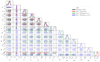 |
Fig. A.2. 1σ and 2σ contours for the parameters ηm and λs for the four models of the 1 keV system in 𝒟1. |
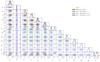 |
Fig. A.3. 1σ and 2σ contours for the parameters ηm and λs for the four models of the 3 keV system in 𝒟1. |
All Tables
Summary of the image acquisition characteristics, and source and lens redshifts of both gravitationally lensed systems studied in this work.
Values of the lens mass distribution fiducial parameters used to create the mock data and prior probability distributions to model it for 𝒟1, 𝒟2, and 𝒟3.
Values of the differences in logarithmic evidence from the nested sampling of the parameters of each model of lens mass distribution for 𝒟1.
All Figures
|
Fig. 1. Power spectra for CDM, mχ = 1 keV and mχ = 3 keV WDM. The WDM power spectra correspond to low-pass filtered versions of the CDM power spectrum. The vertical axis is unitless and arbitrarily normalised. The free-streaming scale is a function of the dark matter particle mass mχ, and is directly related to the cut-off scale. |
| In the text | |
|
Fig. 2. Upper panel: Full projected data from both simulations from R22. Each square has a side length of 8h−1Mpc, and corresponds to a 80h−1 Mpc projection depth. Panel (b) contains fewer small-scale dark matter halos than panel (a) as the free-streaming length is longer in 1 keV than in 3 keV WDM. Lower panel: Non-Halo projected data from both simulations from R22. Each square has a side length of 8h−1Mpc1, and corresponds to a 80h−1Mpc1 projection. Panel (c) contains smoother and less clumpy structures at small scales than panel (d). The markers are all at the same coordinates and show the regions from which we select the non-halo material used as additional perturbations in our gravitationally lensed systems. These correspond to the highest density of non-halo material in both simulations and to the densest halo in both simulations, excluding those which are cut in the top-left corner. |
| In the text | |
|
Fig. 3. 20 × 20 kpc2 maps of the convergence, deflection angle components, and shear components for the non-halo material in two regions around halos at the same coordinates in the 3 keV (top) and 1 keV (bottom) simulations from R22. The deflection angle maps are used to add the effect of non-halo structures on top of the deflection from the elliptical power law lenses in our datasets. The positions of the non-halo material from which we compute these convergence maps are marked in Fig. 2. They are the same in both simulations. The white contours are based on the arc light image of SDSSJ110+3649 propagated from z = 0.733. |
| In the text | |
|
Fig. 4. Left panels: System SDSS J1110+3649. Right panels: System SDSS J1201+4743. The top panels represent the source brightness distribution and the bottom panels represent the observed flux after propagating through the lens, convolving with an HST-type point spread function, and adding a Gaussian noise resulting in a signal to noise ratio of 10. |
| In the text | |
|
Fig. 5. Optimisation results when modelling the three systems from 𝒟1 with an elliptical power law + external shear. The upper panel (a) shows the results for the unperturbed system, the middle panel (b) for 1 keV, and the lower panel (c) for 3 keV. From left to right: images are the initial data, reconstructed model, normalised residuals between these two images, and reconstructed source. The units are arbitrary, but analogous to a 2D mass density |
| In the text | |
|
Fig. 6. 1σ and 2σ contours for the parameters ηm (excluding the center coordinates xc and yc, and the source regularisation λs) for the elliptical power law + external shear model of the unperturbed, 1 keV and 3 keV systems in 𝒟1. The dashed lines show the 2D distributions, the solid lines show the marginal distributions and the dotted grey lines mark the true values. |
| In the text | |
|
Fig. 7. Difference in the sources brightness distribution in the source plane obtained when modelling the systems in 𝒟1 with a lens following an elliptical power law profile with additional external shear. If SX is the source surface brightness distribution obtained for the system X, these images are the result of SUnperturbed − S1 keV (left) and SUnperturbed − S3 keV (right). The local surface brightness of the reconstructed source can be shifted and modified in the perturbed models if some of the additional perturbations are absorbed by variations of the main lens properties. The general trend given by these images is that the main effect of the additional perturbation is an overall shift of the source, which is indicated by corresponding red and blue regions of the 2D brightness distribution. To highlight this effect, the black markers give the point of highest surface brightness (‘+’ for the unperturbed system and ‘x’ for the perturbed one). |
| In the text | |
|
Fig. 8. 1σ and 2σ contours for the parameters ηm for the elliptical power law + external shear model of the unperturbed, 1 keV, and 3 keV systems in 𝒟2. The layout is the same as in Fig. 6. |
| In the text | |
|
Fig. 9. 1σ and 2σ contours for the parameters ηm for the elliptical power law + external shear model of the unperturbed, 1 keV, and 3 keV systems in 𝒟3. The layout is the same as in Fig. 6. |
| In the text | |
|
Fig. 10. 1σ and 2σ contours for the parameters ηm with third and fourth order multi-poles (excluding the center coordinates xc and yc, and the source regularisation λs) for the four models of the 1 keV system in 𝒟1. The reference lens model is the elliptical power law+external shear. |
| In the text | |
|
Fig. A.1. 1σ and 2σ contours for the parameters ηm and λs for the four models of the ’unperturbed’ system in 𝒟1. |
| In the text | |
|
Fig. A.2. 1σ and 2σ contours for the parameters ηm and λs for the four models of the 1 keV system in 𝒟1. |
| In the text | |
|
Fig. A.3. 1σ and 2σ contours for the parameters ηm and λs for the four models of the 3 keV system in 𝒟1. |
| In the text | |
Current usage metrics show cumulative count of Article Views (full-text article views including HTML views, PDF and ePub downloads, according to the available data) and Abstracts Views on Vision4Press platform.
Data correspond to usage on the plateform after 2015. The current usage metrics is available 48-96 hours after online publication and is updated daily on week days.
Initial download of the metrics may take a while.