| Issue |
A&A
Volume 697, May 2025
|
|
|---|---|---|
| Article Number | A210 | |
| Number of page(s) | 17 | |
| Section | Planets, planetary systems, and small bodies | |
| DOI | https://doi.org/10.1051/0004-6361/202453565 | |
| Published online | 21 May 2025 | |
Secular brightness curves of 272 comets
1
Instituto de Astrofísica e Ciências do Espaço, Universidade de Coimbra,
Portugal
2
Laboratoire de Géologie de Lyon: Terre, Planètes, Environnnement, CNRS, UCBL, ENSL,
Villeurbanne,
France
3
Institute of Astronomy and National Astronomical Observatory, Bulgarian Academy of Sciences,
72 Tsarigradsko Chaussee Blvd.,
1784
Sofia,
Bulgaria
4
Dep. Science and Technology, Parthenope University of Naples,
Naples,
Italy
5
INAF – Osservatorio Astronomico di Roma,
Italy
6
The University of Edinburgh,
Edinburgh,
UK
7
Instituto Pedro Nunes,
Coimbra,
Portugal
8
International Space Science Institute,
Bern,
Switzerland
★ Corresponding author: This email address is being protected from spambots. You need JavaScript enabled to view it.
Received:
20
December
2024
Accepted:
24
March
2025
Abstract
Aims. We investigate the brightening behavior of long-period comets as a function of dynamical age, defined by the original reciprocal semimajor axis, 1/a0. Our goal is to test long-standing claims about comet behavior using a large number of available measurements.
Methods. We used a large set of photometric observations to compute and analyze global and local brightening curves for 272 long-period comets. We fit the observed magnitudes with a linear model in log heliocentric distance, from which we derived brightening parameters for each comet. We categorized the sample into dynamically new, intermediate, and old comets, and we compared their brightening behavior. We also examined the relationships between dynamical age and other orbital and physical parameters.
Results. Dynamically new comets are seen to brighten more slowly than old comets, particularly within 3 au from the Sun. The brightening rate of new comets appears to vary with heliocentric distance. New comets are intrinsically brighter than old comets and exhibit a tighter correlation between brightening parameters.
Key words: methods: data analysis / methods: observational / techniques: photometric / catalogs / comets: general / Oort Cloud
© The Authors 2025
 Open Access article, published by EDP Sciences, under the terms of the Creative Commons Attribution License (https://creativecommons.org/licenses/by/4.0), which permits unrestricted use, distribution, and reproduction in any medium, provided the original work is properly cited.
This article is published in open access under the Subscribe to Open model. This email address is being protected from spambots. You need JavaScript enabled to view it. to support open access publication.
1 Introduction
The Oort Cloud is a vast, diffuse spherical shell composed of a trillion icy objects, extending from approximately a few thousand to tens of thousands of astronomical units from the Sun (Oort 1950; Francis 2005). The objects in the Oort Cloud are remnants from the early Solar System that were scattered by planetary encounters and had their inclinations randomized and their perihelia raised far beyond the planetary region by a complex combination of Milky Way tides and perturbations by passing field stars (Heisler & Tremaine 1986; Heisler et al. 1987; Duncan et al. 1987; Higuchi et al. 2007; Higuchi & Kokubo 2015; Pfalzner et al. 2024). The same processes cause some of these objects to return to the inner Solar System, where they manifest as long-period comets (LPCs; Oort 1950; Heisler & Tremaine 1986; Kaib & Quinn 2009).
Oort (1950) identified an overabundance of LPCs on orbits with an extremely low reciprocal semimajor axis, specifically 1/a0 < 0.0001 au−1, where 1/a0 corresponds to the energy of the comet’s orbit. The semimajor axis, a0, refers to the original orbit before planetary perturbations. When comets pass through the planetary region, their orbits are perturbed, primarily by Jupiter, resulting in changes in the reciprocal semimajor axis on the order of ±0.0005 au−1 (van Woerkom 1948). Oort took the observed abundance of 1/a0 values considerably smaller than this perturbation as evidence that these comets were coming into the planetary region for the first time. Such dynamically new comets are interesting because unlike returning LPCs or short-period comets (SPCs), they have experienced minimal solar irradiation since their ejection from the planetary region.
We build on the work of Oort & Schmidt (1951), who first reported photometric differences between dynamically new and returning comets, namely, that new comets brighten more slowly as they approach the Sun than returning comets. Subsequent studies found evidence for the same behavior (Meisel & Morris 1976; Whipple 1978; Meisel & Morris 1982; Green 1995; A’Hearn et al. 1995; Holt et al. 2024), but all used roughly ten times smaller samples or lacked coverage beyond 3 au. In this work, we employ a larger sample of LPCs observed mainly since the mid-1990s and to heliocentric distances beyond Jupiter, analyzing their brightening as they approach the Sun with the goal of testing the aforementioned claims about comet behavior. We specifically examine the secular brightening behavior, setting aside the apparent unpredictability of comets, which often display large variations in behavior over short timescales and between individual objects.
Even though previous studies vary in the details of how they measure comet brightness, they all attempt to track the comet total magnitude, including light reflected by the nucleus and the (mostly dominant) contribution from the coma. Similarly, this study focuses on comet total magnitudes. As described in Section 2, although we use highly heterogeneous data, we follow a uniform strategy to compare brightening rates between comets. Distinct brightening behavior is indicative of differences in the mechanism of comet activity and linked to the physical properties of comet nuclei (Meech & Svoren 2004).
Oort’s grouping of LPCs into new, intermediate, old, and periodic categories based on the original orbit’s reciprocal semimajor axis (see Table 1) remains a useful framework1. New comets are those likely entering the inner Solar System for the first time, intermediate comets are those likely returning after a distant first perihelion, and old comets have likely visited the planetary region multiple times. We may refer to newer comets as encompassing new and intermediate comets or returning comets when referring to intermediate and old comets together. Periodic comets, which are primarily SPCs, are excluded from this study.
The SPCs, defined as having orbital periods less than 200 yr, include both Jupiter-family comets with low-inclination prograde orbits strongly influenced by Jupiter and Halley-type comets with nearly isotropic orbits. Although spacecraft have visited several SPCs, revealing a diversity of physical characteristics and substantial processing of their nuclei (e.g., Keller & Kührt 2020, and references therein), a similar mission to LPCs has yet to be achieved due to the logistical challenges posed by their long-period orbits. The upcoming Comet Interceptor (CI) mission, a joint endeavor by ESA and JAXA, aims to overcome these challenges by pre-positioning a spacecraft at the Sun-Earth Lagrange point L2 so that it is ready to intercept a suitable LPC when discovered (Jones et al. 2024). The target comet for CI will likely be discovered by the Legacy Survey of Space and Time (LSST; Ivezić et al. 2019) to be carried out at the Vera Rubin Observatory at distances well beyond Jupiter (Jones et al. 2024). The mission’s preparation involves studying the detectability of potential targets and predicting their activity at flyby distances based on initial observations.
Oort dynamical groups.
2 Data and methods
This section describes the formalism, data sources, selection criteria, and analytical methods used to investigate the secular brightening behavior of LPCs. Our analysis began with a comprehensive dataset of the over 3000 known LPCs, which was then systematically refined through a series of selection steps based on specific criteria to ensure a robust final sample of comets for analysis. The selection process included ensuring precise orbital solutions, exclusion of unbound comets and fragments, assessing the availability of photometric observations, and application of quality criteria to address data uncertainty and non-uniformity. The details of these steps are provided in the following subsections. This approach allowed us to focus the analysis on a well-defined set of 272 comets, examining their brightening behavior as a function of dynamical age and other orbital parameters.
2.1 Brightening curves
Comets brighten as they approach the Sun and the Earth. The brightening is due to a combination of observing geometry as the comet approaches both the Sun and the Earth and increasing back-scattering cross-section. Comets can be seen in reflected or scattered sunlight, so the apparent brightness increases with the inverse square of both the heliocentric and geocentric distances. However, as comets approach the Sun, sublimation of their nuclei releases dust into an extended coma, increasing the reflective cross-section and leading to a steeper than inversesquare dependence on heliocentric distance. Furthermore, since the coma is not a point source, its apparent area increases as the geocentric distance (Δ) decreases, leading to a shallower than inverse-square dependence on geocentric-distance (the “Delta effect,” e.g., Hughes et al. 1993). Because this effect is small compared to other uncertainties, and in the interest of uniformity of treatment, we ignore it here.
Expressed in magnitudes, the total magnitude (T) of a comet may be approximated by
![Mathematical equation: $\[T=\mathrm{M} 1+5 ~\log~ \Delta+\mathrm{K} 1 ~\log~ r,\]$](/articles/aa/full_html/2025/05/aa53565-24/aa53565-24-eq1.png) (1)
(1)
where r and Δ are the heliocentric and geocentric distances in au, M1 is the total magnitude at r = Δ = 1 au, K1 is the brightening slope in units of magnitude per log astronomical unit, and the factor five assumes the total brightness depends solely on Δ−2. An inverse square dependence on heliocentric distance would imply K1 = 5, but increasing activity for incoming comets results in brightening slopes K1 > 5.
Parameters M1 and K1 are available from the NASA Jet Propulsion Laboratory (JPL) Solar System Dynamics2 (SSD) services for nearly all known comets. For LPCs, K1 varies roughly between 4 and 48, with a median near 10 mag/log(au). The total magnitude parameter, M1, ranges from 4 to 22, with a median value of 10 magnitudes. M1 is akin to the absolute magnitude, H, but applies to the total magnitude of active comets. Its range of validity is important when comparing to other studies.
To remove the geocentric dependence, which oscillates on a shorter timescale than the cometary orbit, we also consider the heliocentric magnitude, T⊙ = T − 5 log(Δ), given by
![Mathematical equation: $\[T_{\odot}=m+k ~\log~ r,\]$](/articles/aa/full_html/2025/05/aa53565-24/aa53565-24-eq2.png) (2)
(2)
where m and k are parameters analogous to M1 and K1 in Eq. (1). In this paper, we use Eq. (2) as the baseline for comparing brightening curves, focusing primarily on the parameter k, which we will refer to as brightening slope. Parameter m is the total heliocentric magnitude at r = 1. The right-hand side of Equation (2) is also commonly written as m + 2.5n log r, where n is referred to as the “activity index” (Hughes 1988; Whipple 1992) or, less commonly, the “photometric index” (Sosa & Fernández 2011) or the “index of variation” (Meisel & Morris 1976). Parameter k can be converted to the activity index as n = k/2.5.
2.2 Orbit quality selection
Using the astropy package astroquery (Ginsburg et al. 2019), we queried the Minor Planet Center (MPC) database to identify comet orbits, specifically selecting LPCs (prefix C/) that include original reciprocal semi-major axis values, 1/a0, and their uncertainties, σ1/a0. The MPC’s 1/a0 values generally agree with those from other sources3, such as the CODE Catalog (Królikowska & Dybczyński 2020) and the Nakano Note website4 by Syuichi Nakano. Despite using more robust orbit calculations (Holt et al. 2024) these catalogs include only a subset of the orbital solutions available from the MPC. To maximize the sample size and ensure internal consistency, we adopted the MPC original orbits. The 1/a0 values were used to classify LPCs into the different Oort groups (see Table 1). We kept new, intermediate and old comets, and excluded periodic and unbound orbits. On the latter, we retained only comets with 1/a0 > 3σ1/a0, ensuring a 3σ confidence level that the orbits are bound (1/a0 > 0). This criterion minimizes the likelihood of including unbound interlopers. Comet fragments were also excluded resulting in a preliminary sample of 787 comets for further inspection.
We subsequently used the JPL SSD Small-Body Database (SBDB) Query API to retrieve additional parameters and associated uncertainties, σ, for each comet, including semi-major axis (a, σa), time of perihelion passage (tp, σtp), perihelion distance (q, σq), eccentricity (e, σe), inclination (i, σi), and the brightening and magnitude parameters (M1 and K1). The latter result from fitting Eq. (1) to all MPC-reported observations. Importantly, in the case of M1 and K1, this is done without distinguishing between incoming and outgoing data (see Section 4.4 for more details).
2.3 Magnitude data selection
To analyze the total magnitude evolution of the comets in the preliminary sample identified in Section 2.2 as they approach the Sun, we obtained magnitude data from the MPC. Using astroquery, we obtained all reported observations for each comet from the MPC observations database5. These include magnitude, but are primarily used to measure the position and motion of the comets. Historically, the magnitude was specified simply as either nuclear (N) or total (T), but recent T magnitude data are often filter-specific. We focused on T magnitudes, considering observations taken through any available filter, but excluding N data. We chose to exclude N magnitudes for two primary reasons. Firstly, our focus is on the brightening behavior due to cometary activity, which can only be reliably accounted for in T magnitudes. Secondly, and more crucially, there is no straightforward way to verify whether the reported N magnitudes have been processed by observers to remove residual coma effects. Such processing, if present, could introduce additional systematic biases into our analysis. By focusing solely on total magnitudes, we aim to maintain consistency and minimize potential sources of systematic error. Comets for which astroquery returned no magnitudes, or only N magnitudes, were filtered out at this stage.
Each MPC observation includes the comet’s designation, the observation date and time, the observed magnitude, the photometry type (T or filter band pass), and the observatory code. We note that MPC magnitude uncertainties are not provided. To address the lack of uncertainty information, we developed a strategy which relies on sequences of consecutive measurements taken by the same observer instead of individual measurements. Each sequence allows determination of slope and respective uncertainty. This strategy is described in Section 2.4.
We used the JPL Horizons File API to retrieve the observing geometry, specifically the heliocentric (r) and geocentric (Δ) distances for each observation. Additionally, we classified each observation as pre-perihelion or post-perihelion based on the observation time relative to the perihelion passage.
The final dataset consists of 247 773 measurements for 741 comets, obtained at 978 different observatories, spanning heliocentric distances from 0.3 to 35 au. Most measurements are from survey observatories, including ATLAS (Smith et al. 2020), Pan-STARRS (Hodapp et al. 2004), the Catalina Sky Survey (Larson et al. 2003), and LINEAR (Stokes et al. 2000). The majority of the data (over 99%) were collected since 1996, thanks to these surveys and contributions from amateur observers at various observatories across Europe, notably at Tarbatness Observatory (Portmahomack, Scotland), Olmen (Balen, Belgium), Obs. Chante-Perdrix (Dauban, France), Brixiis Observatories (Kruibeke, Belgium), and Grömme (Oudsbergen, Belgium). A sample of observations grouped by comet is shown in Figure 1. Table 2 describes the dates and distances of the measurements. The full table of observations is made available online here.
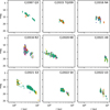 |
Fig. 1 Small subset of observations grouped by comet. Colors correspond to different observatories and symbols to different photometric bands. A larger sample appears in Appendix A. |
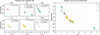 |
Fig. 2 Strands (top panel array) and global curve (bottom panel) for comet C/2019 U6. Top array panels are labeled by MPC observatory code (E89=Geyserland, F51=Pan-STARRS 1, Q38=Lake Boga, T05=ATLAS-HKO, T08=ATLS-MLO, W88=Slooh). Top-panel legends indicate strand filter and whether strands are valid or invalid, the latter indicated as the reason for rejection. Global curve legend indicates filter (same symbols as top array panels), for comparison. We note that the global curve may include points from invalid strands, e.g., green diamonds in top sub-panel F51, which means they were not useful to assess local slope, but are useful to assess the global behavior. |
Date and geometry of observations analyzed.
2.4 Robust brightening measurement using strands
The MPC magnitude data described above were collected mainly for astrometry and orbit determination and hence the lack of photometric uncertainties. Furthermore, comet photometry is inherently complex (Jewitt 1991) and is often influenced by subjective factors, which are not detailed for the MPC observations used in this study. Variations in observational techniques (e.g., aperture selection, different filters) may introduce magnitude offsets between observatories. As a result, the data for each comet are highly heterogeneous, presenting significant challenges for analysis. To address these challenges, we introduce “strands”: sequences of consecutive measurements taken by the same observatory using the same filter. It may be helpful to inspect Figure 2 for a visual representation of strands.
We fitted Eq. (2) to separate strands, to extract their slope and magnitude parameters, which we will denote kr and mr. A key advantage of this approach is that strand-based slopes (kr) are robust to differences between observers and to color offsets because each strand is derived from a single filter at a given observatory, and their slope depends only on relative changes within a single strand. This ensures that the brightening trends we extract are as free as possible from systematic observational biases. Each strand also provides an uncertainty estimate on kr and mr, denoted σkr and σmr, allowing us to assess the quality of the data and filter out unreliable strands (discussed in the next subsection). We note that mr is still susceptible to variations in observational techniques, such as aperture selection or calibration inconsistencies, so its interpretation requires more caution.
In the subsequent analysis, strands serve as the fundamental building blocks for studying the comet’s brightening behavior. Another important benefit of strands is that they represent different heliocentric distances; this is highlighted by the subscript r in kr and mr. As will become clear below, this enables us to measure changes in brightening rate with heliocentric distance.
2.5 Strand quality selection
To ensure that strand-based brightening rate measurements are reliable, we first applied a set of selection criteria before performing any slope fitting. The fundamental requirement is that a strand must provide a reliable estimate of the brightening slope, kr. If a strand lacks sufficient data points, does not span a sufficient range in heliocentric distance, or consists primarily of clustered measurements at its extremities, its slope may be misleading. Thus, to be considered reliable, a strand must satisfy the following conditions:
It should contain at least ten individual measurements.
It should span at least 0.5 au in heliocentric distance.
Its measurements should be well-distributed in heliocentric distance, rather than forming isolated clusters at the extremities. This was enforced by binning the data into five equal intervals in log r and requiring at least one measurement outside bins 1 and 5.
These particular criteria are based on extensive visual and numerical inspection of the resulting fits. Strands with fewer measurements or insufficiently broad or bimodal coverage often yielded fits that, while sometimes statistically acceptable, did not reliably reflect the comet’s secular brightening trend. More complex, adaptable criteria, produced equivalent results, so we opted to use a simpler and more easily reproducible set of thresholds.
Our focus is on the secular behavior of comets, so we evaluated strands based on the expectation of regular brightening, excluding data that did not conform to this pattern. By “regular brightening,” we mean that a comet’s brightness should vary according to Eq. (2). Spurious data would introduce scatter that disrupts this smooth trend. Thus, to assess each comet’s secular brightening, we aimed to reject data that exhibit excessive scatter. Although comet outbursts can complicate this assessment, filtering out such events is acceptable, as this study focuses on long-term brightening trends.
As such, we subjected strands that meet the criteria above to an ordinary least squares (OLS) fit to Eq. (2), and used the F-test p-value to reject the null hypothesis that all fit parameters are zero, that is, the strand magnitudes are consistent with noise. The F-test is well established and easy interpret when assessing linearity; a large p-value indicates that Eq. (2) has no explanatory power regarding the strand magnitudes. Only strands with pval < 0.0027 (3σ) and kr uncertainties σkr < 1 were considered valid.
Number of strands, global curves, and comets analyzed.
2.6 Extraction of strand brightening parameters
We extracted the brightening parameters mr and kr and respective uncertainties by fitting Eq. (2) to each of the valid strands using a robust linear model (RLM6). We chose to use RLM to extract the brightening parameters for analysis because it is more effective in capturing the main slope in the presence of outliers. We entertained the possibility that differences in number and density of measurements per strand could affect the robustness of their respective kr values, but tests involving the most extreme cases showed no significant deviation from the initial RLM fits.
Finally, each strand was associated with its comet, observatory, and photometric band, along with the comet’s original orbital properties, perihelion, and discovery information. Additionally, the strand’s specific properties, including number of measurements, minimum and maximum heliocentric distances (r), midpoint in log r, and best-fit parameters kr and mr, were recorded.
2.7 Global curves
To further understand the overall brightening trends of each comet, we performed two additional Eq. (2) fits per comet: one using all pre-perihelion data and the other using all post-perihelion data, irrespective of the observatory or photometric band. These “global fits” and associated best-fit parameters, which we will denote k1 and m1, allowed us to measure the overall slope of each comet’s brightening curve. Valid global curves were also required a minimum of 10 measurements covering at least 0.5 au in a relatively uniform manner, the same fit quality criteria as individual strands, and the inclusion of at least two strands.
Number of comets per orbital arc, Oort group, and strand count.
Heliocentric coverage (in au) of strands.
2.8 Sample summary and debiasing
The resulting sample includes 272 comets, 176 with both valid strands and global curves, 78 with global curves but no valid strands and 18 with valid strands but no global curves. In total, 992 strands were deemed fit for analysis, corresponding to 194 comets. Approximately one-third of the comets have only a single strand, with a median of two strands per comet, and a maximum of 67 strands for comet C/2017 K2. Most of the strands are pre-perihelion (644) compared to post-perihelion (348). As for global curves, 254 comets have valid coverage of either pre-perihelion brightening or post-perihelion fading, while 92 comets have both pre- and post-perihelion global curves. Tables 3 and 4 summarize how comets, strands and global curves distribute over orbital arc and Oort group. Figure 3 shows the distribution of 1/a0 for global curves and strands. Figure 4 and Table 5 show how strands are distributed in heliocentric distance. The resulting table of strands and global curves and their properties is made available online here.
In the specific case of strands, the sample summarized above is biased because some comets contribute more strands than others. We could address this problem by randomly resampling the strand sample ensuring each comet contributes the same amount of strands. However, this would lead to uneven coverage of heliocentric distance. As we will see below, the brightening slope, kr, appears to vary with heliocentric distance, making it important to ensure that all distance ranges are evenly represented. To address the biases, we first binned strands according to their midpoint in log heliocentric distance, which serves as an anchor for each strand when modeled using Eq. (2). The bin boundaries were set at 2, 3, 4, 5 and 6, extending indefinitely at both ends, attempting uniform coverage of the range containing the most data. We experimented with different bin structures, but found no significant impact in the results as long as each bin contains at least 30 strands. Next, we randomly sampled (with replacement) an equal number of strands from each bin, while simultaneously ensuring each comet contributes the same amount of strands. As an example for the case of pre-perihelion strands, we selected 107 or 108 strands per bin, ensuring that the total number of resampled strands remains 644. In the bin nearest the Sun, we drew 5 or 6 strands for each of the 18 comets, obtaining a total of 107 resampled strands for the bin (see Figure 4). The resulting samples, which we will refer to as “debiased strand samples,” are a fairer representation of the variability due to individual comets and heliocentric distances.
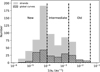 |
Fig. 3 Distribution of 1/a0 for strands (multiple per comet) and global curves (one or two per comet). Oort group ranges are identified. |
3 Results
3.1 Comparing Oort groups using bootstrap
To assess whether the photometric behaviors of new, intermediate, and old comets differ, we compared their brightening parameters by testing the null hypothesis that they are drawn from the same parent population. Using the debiased strand samples described above, we compiled kr and mr distributions for each Oort group, both pre- and post-perihelion. Since global curves do not require debiasing, we used used the k1 and m1 samples directly.
We then applied bootstrap resampling to evaluate how often the observed differences between two Oort groups could arise by chance. Specifically, we constructed synthetic samples by randomly shuffling Oort group labels and re-computing the difference multiple times. This allowed us to estimate the probability (p-value) that a difference as large as the observed one would occur if the groups were inherently indistinguishable, ensuring robustness to sample size. We adopt a 3σ significance threshold, considering results statistically significant if pval < 0.0027.
To quantify the differences between samples, we used the Kolmogorov-Smirnov D statistic7 (DKS), which measures the maximum difference between the respective cumulative distributions. DKS is equal to zero when the compared distributions are identical, and increases as they diverge in location, scale, or shape. Our bootstrap approach and choice of metric are nonparametric as we are dealing with asymmetric distributions, and is robust to sample size. Since debiased strand samples are drawn at random from the original sample, which introduces variability, we generated multiple (Ni) instances and averaged the results to obtain stable estimates of statistical properties and p-values. We found that Ni = 100 was sufficient achieve convergence.
3.2 Comparing brightening using strands
Figure 5 shows cumulative distributions and histograms of the kr parameter, grouped by Oort group, and Table 6 details the statistical properties of each distribution. We subjected each debiased kr sample to the bootstrap resampling described at the start of this section to calculate the p-values for the null hypothesis that the samples being compared are drawn from the same parent population. These are shown in Table 7, where each p-value is the average of Ni = 100 debiased strand samples.
The distributions of brightening slopes for strands of new and intermediate comets are not significantly different (pval ≈ 0.15), both groups having median kr near 11.1 to 11.3 mag/log(au). In contrast, old comets display markedly different behavior, characterized by a higher median kr = 13.2 and a distribution skewed to larger kr, lacking comets that brighten very slowly. The kr distribution for old comets differs significantly from both new comets (pval = 0.0019) and intermediate comets (pval = 0.0014). Although Oort & Schmidt (1951) use a different parametrization of brightening with heliocentric distance (for details, see Meisel 1970), our results corroborate their primary conclusion that new comets display different photometric behavior, brightening more slowly as they approach the Sun than old comets.
3.3 Comparing brightening using global curves
Analyzing the k1 distributions for global curves reveals a similar trend, though the differences between the Oort groups are less pronounced (see Figure 6, and Tables 7 and 8). The smallest p-value occurs when comparing new and old comets (pval ≈ 0.03). New and intermediate comets are statistically indistinguishable (pval ≈ 0.45), as are intermediate and old comets (pval ≈ 0.23). New comets have the lowest brightening slope (median k1 = 12.3, interquartile range IQR = 5.7), followed by intermediate comets (median k1 = 12.8, IQR = 7.1) and old comets (median k1 = 14.8, IQR = 8.6). The reduced distinction among global curves could be attributed to the smaller sample sizes; however, as discussed below, it may also be caused by trying to capture the brightening with a single set of parameters for all heliocentric distances.
We note here that the brightening parameter K1, easily accessible from the SBDB, already hints at the same differences in behavior. New comets have the narrowest distribution and the lowest median K1 = 6.5, with an interquartile range (IQR) between 4.6 and 8.9. Old comets have the broadest distribution and the steepest brightening (median K1 = 9.5, IQR [6.4, 14.3]) and intermediate comets have intermediate brightening (median K1 = 7.8, IQR [5.4, 10.3]). If we take all three dynamical groups together, K1 has a median of 7.5, with IQR [5.3, 10.3].
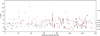 |
Fig. 4 Distribution of strands into comets and over heliocentric distance. Pre-perihelion strand midpoints (vertical axis) are plotted as open circles for each comet (horizontal axis) in the original sample (644 strands for 141 comets). Horizontal dotted lines mark heliocentric bin boundaries. Numbers of strands and comets in each bin in the original sample are shown separated by a slash to the right of the Figure. A debiased strand sample (see text for details) is overplotted as red dots. |
Strand parameter statistics by Oort group and orbital arc.
3.4 Evolution of brightening slope with heliocentric distance
To evaluate potential changes in brightening behavior with heliocentric distance, we analyzed separately strands that lie entirely within (interior) or beyond (exterior) a specific heliocentric distance. As before, we used debiased strand samples, ensuring that each distance range and each comet contribute the same number of strands. Figure 7 illustrates the contrast between the kr distributions of interior and exterior strands for a range of distance boundaries.
Focusing on the boundary at 3 au, we find that new comets have significantly different kr medians inside and outside that distance (6.7 versus 12.8, respectively). According to the Wilcoxon-Mann-Whitney U test, the null hypothesis that the medians are equal is rejected with pval ~ 10−4. For intermediate comets, the difference is notable but smaller (medians 7.8 versus 12.5, pval = 0.022), and does not reach the 3σ significance threshold. Furthermore, the range of boundaries in Figure 7 suggests that both groups experience a steady decline in brightening rate, from ≳12.5 to less than 10 mag/log(au), as they approach the Sun. In contrast, the brightening slope of old comets shows no significant difference inside and outside 3 au (medians 13.4 versus 14.6, pval = 0.45) and exhibits larger scatter. We note that using a smaller but more homogeneous sample of 21 LPCs, Holt et al. (2024) also find a decreasing rate of brightening as comets approach the Sun. Their sample is dominated by new comets, with only 3 returning LPCs.
Additionally, both Figure 7 and the median values suggest that the brightening behavior of newer and old comets differs primarily within 3 au. The U test confirms this, rejecting the null hypothesis when comparing the medians of new and old comets inside 3 au (pval ~ 10−6). The difference between intermediate and old comets is less pronounced (pval = 0.02), falling short of the 3σ threshold. Outside 3 au, the same test indicates that all three groups have statistically indistinguishable medians (pval ≥ 0.27).
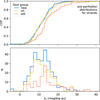 |
Fig. 5 Cumulative probability distributions (top) and histograms (bottom) of the kr brightening parameter for pre-perihelion strands, by Oort group. Shown are averages of Ni = 100 debiased strand sample distributions (see text for details). Histogram counts were rescaled so that they add up to the actual number of pre-perihelion strands measured. |
Bootstrap comparisons of strand and global curve parameters across Oort groups and orbital arcs.
3.5 Testing non-linear brightening models
If indeed the slopes of strands vary with heliocentric distance, global curves are unlikely to follow a strictly linear relationship as prescribed in Eq. (2). To test this, we compared the original linear fit with a quadratic fit in log r using OLS fitting and the Akaike Information Criterion (AIC), as implemented in Python’s statsmodels package. AIC accounts for both the goodness of fit (through the likelihood function) and model complexity (via a penalty for additional parameters). As anticipated, 83.8% of global curves are better represented by a quadratic model. Interestingly, strands are also more accurately described by a quadratic fit: 68.9% favor a quadratic model, while 31.1% are better explained by a linear fit. As expected, the difference is less pronounced, given that strands cover narrower heliocentric ranges. Further analysis of the fit residuals (normality, mean, skew and homoscedasticity) for the two models confirmed the conclusion offered by AIC. Improving the modeling of secular brightening requires a more uniform sample, for instance focusing on data from the best characterized surveys. Snodgrass & Holt (2024) found evidence for non-linear brightening in LPCs and propose an alternative empirical model where the rate of brightening varies linearly with heliocentric distance.
3.6 Post-perihelion fading behavior
If we look at the post-perihelion fading behavior, we find that it is more consistent among the different Oort groups (see Figures 8 and 9 and Tables 6 and 8). Parameter kr (now a fading slope) for outgoing strands of newer comets tends to be slightly shallower than that of old comets; however, the distributions are not significantly different (see Table 7). Moreover, the fading slope samples of outgoing global curves of new, intermediate and old comets are statistically indistinguishable (Table 8).
For the 92 comets with both incoming and outgoing data, Figure 10 compares the global curve pre- and post-perihelion, illustrating how the k1 slope changes between brightening and fading (see also Table 9). The median change in slope is Δk1 = −0.6 mag/log(au) and the number of comets that increase or decrease kr after perihelion is roughly equal. Half of comets exhibit slope changes within −3.3 < Δk1 < 2.0 mag/log(au). Figure 10 suggests a correlation between Δk1 and incoming k1, particularly for newer comets. A robust linear fit yields the relation Δk1 = −0.65(k1 − 11.6). If the post-perihelion fading slope is related to the subsequent pre-perihelion brightening, the apparent trend would lead to k1 converging toward a value near 11.6 mag/log(au) after repeated perihelion visits.
Statistics of global curves k1 and m1 samples.
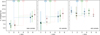 |
Fig. 7 Brightening slope of strands as a function of heliocentric distance. A range of distance boundaries, shown as vertical dotted lines labeled by distance, separate strands into interior and exterior to the boundary. Two horizontal lines extending from each boundary to the left and to the right connect to boxes that correspond to interior and exterior strands, respectively. The x coordinate of each box is the median of the midpoint in log r of the strands. The y extent of each box contains the IQR of the kr distribution. Inside each box, a horizontal line marks the median and a star symbol indicates the mean of the kr distribution. |
3.7 Investigating the m1 parameter
As mentioned above, mr and m1 are less reliably extracted from the MPC data due to inconsistencies in the photometric analysis by different observers. Furthermore, the aforementioned changes in kr as the comet approaches the Sun imply that mr fits to strands will depend on heliocentric distance. This is apparent in Figure 11, where mr values increase as comets approach the Sun, reflecting the corresponding decrease in kr. It is reassuring that the m1 values obtained from fitting global curves (to the left of the dashed line in the figure) are consistent with the values of kr for strands approaching 1 au (right of dashed line). With these caveats in mind, we compare in Figure 12 the distributions of the m1 parameter for new, intermediate, and old comets. New comets exhibit brighter median m1 values than old comets (Table 8), and the respective distributions are statistically incompatible according to the bootstrap test (pval = 0.0015, Table 7). The m1 distributions for intermediate and old comets are not incompatible at the 3σ level (pval = 0.0135), and new and intermediate comets are indistinguishable (pval = 0.5). In Section 4.2 we discuss the possibility that the brighter median m1 for new comets when compared to old comets is the result of a selection bias.
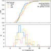 |
Fig. 9 Same as Figure 6 but for the k1 fading parameter corresponding to post-perihelion global curves. |
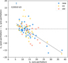 |
Fig. 10 Difference between brightening and fading slopes of global curves. A robust linear model fit of the form Δk1 = −0.65(k1 − 11.6) is shown (adjusted R2 = 0.27). |
Brightening/fading slope change statistics.
3.8 The link between the brightening parameters
The link between mr and kr for strands is straightforward since they are derived from local fits. However, it is interesting to examine the relationship between m1 and k1 for global curves, as it captures secular trends in brightening behavior. Figure 13 illustrates this relation for pre-perihelion global curves, grouped by Oort group. Linear fits are also shown, together with analytical expressions and coefficients of determination, R2. The slopes of these fits are close to −1, particularly for new comets. The fit is tightest for new comets, yielding residuals with a median of −0.1 and an IQR of [−1.6, 1.6], and intermediate comets (median: −0.2, IQR: [−1.7, 1.8]). For old comets the residuals become more dispersed (median: −0.5, IQR: [−3.2, 2.6]). To assess whether the dispersion of residuals differs between dynamical groups, we applied the Fligner-Killeen test, a non-parametric method robust to non-normality that ranks absolute deviations from the median. We compared the residuals of new versus old and intermediate versus old comets, testing the null hypothesis that their dispersions are equal. The test yielded pval ~ 10−5 for new versus old, indicating a highly significant difference. For intermediate versus old, we obtained pval = 0.00145, which is still significant at 3σ significance. In the case of new comets, the approximate constancy of m1 + 1.01k1 suggests that these comets have similar magnitudes at r ≈ 101.01 ≈ 10.2 au. This uniformity of behavior is intriguing, and may be influenced by a selection bias. However, while the absence of new comets with fainter m1 can be explained in this context, the lack of examples with steeper k1 values remains unexplained. A more detailed analysis of this trend is beyond the scope of this paper, but determining its underlying cause will likely require a well-characterized survey such as LSST.
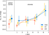 |
Fig. 11 Median mr for strands as a function of heliocentric distance and Oort group (shown to the right of the vertical dashed line). Strands are binned in equal-sized rmin bins (linear r), and the median mr and median absolute deviation are plotted as points and error bars, respectively. Bin centers coincide with the x-axis location of the “int.” symbols and the “new” and “old” symbols where horizontally nudged for clarity. To the left of the vertical dashed line are the m1 distribution median plus or minus the mean absolute deviation for global curves. |
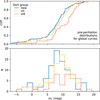 |
Fig. 12 Empirical cumulative probability distribution of the m1 parameter for pre-perihelion global curves organized by Oort group. |
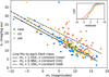 |
Fig. 13 Relation between m1 and k1 for pre-perihelion global curves, color-coded by Oort group. Points correspond to individual comets. Black lines are RLM fits to each Oort group. The respective fit coefficients of determination are |
![Mathematical equation: $\[R_{\text {new }}^{2}=0.71, R_{\text {int }}^{2}=0.71\]$](/articles/aa/full_html/2025/05/aa53565-24/aa53565-24-eq3.png)
![Mathematical equation: $\[R_{\text {old }}^{2}=0.45\]$](/articles/aa/full_html/2025/05/aa53565-24/aa53565-24-eq4.png)
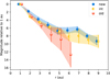 |
Fig. 14 Average relative magnitude brightening per Oort group. Median magnitudes are calculated for each comet in heliocentric distance bins, grouped by Oort classification and averaged. See text for details. Shading connecting points and 1σ standard error bars are added to guide the eye. Bin centers coincide with the x-axis location of the “int.” symbols and the “new” and “old” symbols where horizontally nudged for clarity. |
3.9 Brightening trends from direct magnitude analysis
As an alternative to modeling the reported magnitudes using Eq. (2), we can directly analyze the magnitudes to identify trends in brightening behavior. Figure 14 shows how the magnitude of incoming comets, relative to their magnitude at 1 au, varies with heliocentric distance. To generate these curves, we consider only comets that reach 1 au and divide each comet’s measurements into heliocentric distance bins (1 au wide and 1 au apart, centered at 1, 2, 3, ... au). For each bin, we compute the median magnitude and subtract the median magnitude at 1 au to produce a relative brightening curve for each comet. We then derive average brightening curves for each Oort group by computing the mean and standard deviation in each bin. The resulting values, along with quantiles of the brightening distribution in each bin, are listed in Table 10. These results confirm that newer comets brighten more gradually as they approach the Sun, while old comet display more scatter and no data beyond r ≈ 6 au. As a general trend, inbound new and intermediate comets brighten by approximately 10 magnitudes between 10 au and 1 au. We note that these brightening trends are based on a limited number of comets (see Table 10).
Magnitude brightening distribution as a function of heliocentric distance organized by Oort group.
3.10 Trends with other orbital elements
The orbital inclination distributions of new, intermediate and old comets in our sample are similar and all uniform between 0 and 180 degrees. Likewise, orbital inclination does not seem to influence the k1 distribution: no trends are observed between the two, either overall or within individual Oort groups. However, perihelion distance and Oort group are linked in our sample: new comets have a larger median perihelion distance (qnew = 3.1 au) compared to intermediate comets (qint = 2.8 au) and old comets (qold = 1.8 au).
Meisel & Morris (1976) noted that splitting comets by perihelion distance results in a stronger distinction than using 1/a0. Specifically, they divided comets into two groups: those with perihelion distances inside and outside q = 1.25 au. Their choice of threshold was partly constrained by the limited number of comets in their sample with q > 3 au and the absence of any with q > 3.8 au. Given that our dataset includes a larger number of high-perihelion comets, we investigated whether splitting the sample at a larger q would yield a greater difference in brightening behavior. Using the bootstrap procedure described at the start of this section, we tested qsplit from 1 to 4 au in steps of 0.25 and found no significant difference between kr interior and exterior to any value of qsplit.
4 Discussion
We found evidence that new comets behave differently from returning comets as they approach the Sun. The main differences are that newer comets are typically brighter at all distances (Figures 12 and 14), brighten more slowly, particulary inside 3 au (Figures 5 and 7), and display a tighter correlation between m1 and k1 (Figure 13) than old comets. Intermediate comets display intermediate behavior, which tends to be closer to that of new comets. The different distributions for the brightening slope are most obvious when calculated for individual strands (kr) which capture the effects of changing slope with heliocentric distance (Figure 5.) We discuss these points below.
4.1 On the different brightening of new and returning comets
A number of authors have found that new comets show a slower increase in brightness as they approach the Sun (Oort & Schmidt 1951; Meisel & Morris 1976; Whipple 1978; Green 1995). Our analysis uses a much larger set of comets and essentially confirms this result, while adding that the brightening slope of new comets decreases from kr ≈ 13 mag/log(au) beyond 3 au to kr ≈ 7 mag/log(au) inside 3 au, where it plateaus (see Figure 7). Converting Eq. (2) to total flux relative to 1 au, these translate into r−kr/2.5, that is, an approximately r−3 dependence inside 3 au, which rises to approximately r−5 and even steeper beyond that distance. This slowing rate of brightening is corroborated by a recent dedicated observing campaign, which collected data on 21 LPCs and using the Las Cumbres Observatory network of telescopes (Holt et al. 2024). Despite being smaller in number, their observations were calibrated and processed in a uniform manner, resulting in high quality data that also show that LPC secular brightening is not adequately described by Eq. (2) with a single set of parameters from beyond Jupiter all the way to perihelion. Even though the authors report no difference between the behavior of new and returning comets, their sample included only 3 returning comets, so we interpret it as representative of new comets.
Qualitatively, the behavior of newer comets fits with a proposed explanation (Whipple 1978) that the availability of hypervolatile ices driving their activity is exhausted before they reach perihelion because those ices are concentrated on a thin, near-surface, “frosting” layer developed by cosmic ray irradiation in the Oort cloud over the age of the Solar System. The release of ices in order of decreasing volatility (e.g., Delsemme 1982; Meech & Svoren 2004) results in a decreasing rate of brightening, ending with the least volatile available ice, of which the value kr ≈ 7.5 mag/log(au) is representative (see Figure 7). Repeated perihelion visits lead to progressive build-up of a patchy mantle of refractory material mixed with low volatility ices. As the fraction of the surface covered by this mantle increases, irregularities in thickness and spatial distribution may explain the larger, more scattered and less r-dependent kr of old comets.
New and intermediate comets behave similarly inside 3 au, but new comets brighten more slowly than even intermediate comets at distances 4–7 au. This suggests that the exhaustion or severe depletion of hypervolatiles in new comets occurs further out, consistent with activity starting at large distances (Jewitt et al. 2021), even though CO has been detected in C/2017 K2 at 6.7 au (Yang et al. 2021) and CO, CH3 and CH3OH have been detected in C/2007 N3 at 1.3 au (Dello Russo et al. 2016), both dynamically new comets. Detailed observations and modeling of the activity of the well-studied C/2017 K2 exemplify the intricacies of decoding the interplay of different physical mechanisms (e.g., Jewitt et al. 2019; Fulle et al. 2020; Bouziani & Jewitt 2022). Such an effort is beyond the scope of this paper.
The differences between the photometric behavior of new and returning comets have been highlighted as a possible explanation for the odd proportion of new to returning comets, in that the former is several times larger than would be expected from a semi-stationary state where orbits evolve toward smaller semimajor axis with repeated visits (Oort 1950; Wiegert & Tremaine 1999). This lack of returning comets is generally explained by strong “fading” of comets following their first return to the planetary system from the Oort cloud, which may begin beyond Neptune (Kaib 2022). The progressive change in brightening behavior we observe from new, to intermediate, to old comets supports the idea of evolution in the direction of fading as a result of repeated perihelion visits. The subjacent cause of the fading is not identified with certainty and may be due to a combination of effects. For instance, activity driven torques may spin-up the nuclei of comets to rotational disruption (Jewitt 2022). This effect is strongly dependent on perihelion distance, which does diminish as comets evolve from dynamically new to old (see Section 3.10, and Kaib & Quinn 2009).
4.2 On the intrinsic brightness of new comets
A study of distant activity of 50 LPCs found that new comets display a higher level of activity than returning comets (Sárneczky et al. 2016). This result, based on observations obtained at a single observatory and subject to uniform processing, is supported by our larger albeit less uniform study: we, too, find that new comets are generally brighter than intermediate comets, which are, in turn, brighter than old comets (Table 8 and Figures 11 and 12). A trend of decreasing intrinsic activity brightness with increasing dynamical ages suggests that it may be related to the cumulative effect of multiple perihelion passages. Indeed, SPCs tend to have fainter total absolute magnitudes and lower activity than LPCs as a whole (e.g., Betzler et al. 2023).
One possible concern is that the observed brightness difference between new and old comets could be the result of a selection bias. However, we believe this is unlikely. In our sample, new comets have a larger median perihelion distance than old comets (qnew = 3.1 au versus qold = 1.8 au). Although new comets would be expected to brighten by approximately 1.1 mag over this range (Table 10), the observed difference in median m1 between new and old comets is 3.3 mag (Table 8), suggesting that selection effects alone cannot account for the observed trend.
The total brightness of an active comet is typically dominated by the coma, which scales with nucleus size assuming the same activity level per surface area (Fernández et al. 1999; Sosa & Fernández 2011; Jewitt 2022). So, one explanation for the observed trend is that new comets possess larger nuclei. This is expected, as comets lose mass due to sublimation and splitting, which affects new comets more frequently than returning ones, and will result in an overall decrease in average size for returning comets compared with new ones (Weissman 1980). Alternatively, dynamically new comets may appear brighter due to intrinsically higher activity levels than those of older, recurrent comets (e.g., Mazzotta Epifani et al. 2014), possibly as a result of higher availability of surface volatiles (Sárneczky et al. 2016). The trend is also broadly consistent with the traditional concept of mantling. In this scenario, a non-volatile mantle of refractory material develops over successive perihelion passages, reducing sublimation and leading to progressively lower activity, eventually resulting in a dormant or extinct comet. It is also possible that all these factors contribute to the observed brightness differences.
To investigate the effect of nucleus size, we used two independent sources of data. Robinson et al. (2024) compiled a set of LPC nucleus size estimates, most of which were obtained using NEOWISE infrared data (Bauer et al. 2017) from the WISE mission (Mainzer et al. 2011). Of those, 18 overlap with our comet data, which we restricted to comets with known Oort group and inbound global curve parameters k1 and m1. For the overlapping LPCs, we find that new comets are generally larger (median r = 8.1 km, N = 7) than intermediate (median r = 4.8 km, N = 6) and old comets (median r = 4.0 km, N = 5). Jewitt (2022) published a sample of LPC sizes derived from total production rates and from non-gravitational acceleration data. The two independent methods they used produce consistent size estimates, which are averaged to produce a list of comet nucleus sizes that partly intersects with our data. Here, too, we find that new comets are generally larger (median r = 1.6 km, N = 6) than intermediate (median r = 1.1 km, N = 6) and old comets (median r = 1.0 km and N = 5). Conveniently, this sample includes radii smaller than that of Bauer et al. (2017), allowing us to extend the scope of our analysis. Combining both sources for nucleus size, we retain the trend: new comets are larger (median r = 4.5 km with IQR 1.7 < r < 8.4 km), followed by intermediate comets (median r = 3.1 km with IQR 1.7 < r < 5.0 km) and old comets (median r = 2.5 km with IQR 1.0 < r < 4.0 km). It is interesting that intermediate comets lie closer to old comets, consistent with most mass loss occurring in the first few perihelion passages. We find no relation between inbound global curve brightening slope k1 and nucleus radius. The Spearman Rank Correlation (SPR) test assigns a pval = 0.854 to the correlation. However, as expected, nucleus size does appear to correlate with the m1 parameter (SPR test pval = 0.017). It is important to note that we are dealing with small samples, resulting in low statistical power, which lowers the chance to detect real features, and potential susceptibility to outliers affecting the results.
To assess the influence of composition, we rely on Robinson et al. (2024) who identified a significant log-log linear correlation between nucleus size and CO/H2O coma abundance. The authors posit that this trend supports a semi-empirical model of near-surface volatile re-entrapment driven by early radiogenic heating (Malamud et al. 2022). This model proposes that larger nuclei, able to retain radiogenic heat, experienced volatile migration to outer layers, leading to a differentiated volatile distribution that sustains activity over multiple perihelion passages, particularly in younger comets. Smaller nuclei, with lower heat retention, would have limited, undifferentiated volatile reservoirs, leading to a stable but lower CO/H2O ratio and a decline in activity with age. The model predicts that dynamically younger comets should be larger and display higher CO/H2O abundances and greater activity. Although Robinson’s sample primarily includes SPCs, it contains some overlap with the LPCs studied here. Using their composition data, we find that new comets show lower CO/H2O abundances (median CO/H2O = 0.10, N = 3) compared to intermediate (median CO/H2O = 0.21, N = 2) and old comets (median CO/H2O = 0.15, N = 2), which opposes the expected trend. Interestingly, Harrington Pinto et al. (2022) find an increasing CO production with increasing 1/a0, that is, with dynamical age. Their interpretation is that a 4.5 Gyr exposure to cosmic-rays in the Oort cloud leads to the erosion of all the near-surface CO, leaving almost none available to sublimate during a first perihelion passage (Maggiolo et al. 2020). Return passages will increasingly expose CO that was buried, increasing its relative importance to activity.
We also examined the potential relationship between CO/H2O abundance and brightening slope. To explore this, we analyzed the kr values of strands nearest in time to the gas abundances measurements. Figure 15 illustrates this relationship, suggesting that higher CO/H2O abundances tend to correspond with smaller brightening slopes. However, the SPR test yielded a pval = 0.09, indicating a lack of statistical significance. We reiterate the caution above, that this discussion is based on very small numbers. More observations are needed to test model predictions in a compelling manner.
Despite the small sample size, these findings suggest that the higher intrinsic brightness of dynamically new comets is more likely associated with larger nucleus size. We tentatively refute Malamud et al. (2022)’s prediction regarding hypervolatile abundances and dynamical age, but this may be due to small-sample statistics. However, we note that A’Hearn et al. (1995) similarly found no dependence of composition on dynamical age, nor evidence for differentiated nuclei. The thermal processing of the layer contributing to the observed activity needs to be further investigated as discussed below.
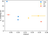 |
Fig. 15 Relation between the brightening slope k1 of global curves and CO/H2O abundance in the coma. |
4.3 On the uniform behavior in new comets
Figure 13 suggests that new comets display tighter correlations between m1 and k1 than old comets. This is supported by the linear fit R2 values listed in the caption, and by analysis of the residuals (see Section 3.8). The brightening parameters for global curves of new comets are such that m1 + 1.01k1 ~ constant. Such a relationship would imply that these comets have a similar magnitude around 10 au. One possibility is that this is the result of a discovery bias, where known new comets are the brightest members of the underlying population. However, this does not readily explain the paucity of new comets with k1 values steeper than those lying on the m1-k1 relation (see Figure 13). If not due to a selection bias, the simplest explanation for this uniformity is that the layer contributing to the activity of dynamically new comets is similar in active area (or size) and composition as they enter the region of giant planets. Figure 14, which shows the average magnitude of comets at different distances relative to 1 au, qualitatively supports the notion that new comets display more uniform behavior than old comets.
The regular behavior of dynamically new comets has been noted previously. In their observational study of 50 LPCs beyond 5.2 au Sárneczky et al. (2016) found that dynamically new comets tend to exhibit more regular and smoothly evolving dust production, with more symmetrical comae, suggesting a more isotropic outflow compared to returning comets. They also observed that dynamically young comets are intrinsically brighter, displaying dust activity at large distances, which they interpret as an indication of uniformity in the initial composition and activity of new comets.
It is plausible that nuclei sent to the Oort cloud early in the Solar System’s evolution, now returning for the first time, underwent uniform processing distinct from that of their dynamically evolved counterparts. If these nuclei also had similar initial compositions and sizes, they might behave more consistently upon their first return to the inner Solar System. However, it remains difficult to explain how spin-axis obliquity, an important factor in controlling activity (Whipple 1978; Marshall et al. 2019), could be made uniform. This likely remains a source of variability in activity patterns between comets. Since spin-axis orientation is believed to cause strong pre-/post-perihelion activity asymmetries (Marshall et al. 2019), the fact that we find roughly equal numbers of comets with decreasing and increasing brightening rates past perihelion argues for randomly oriented spin axes.
Early thermal processing of LPC nuclei before ejection to the Oort Cloud may also introduce variation. Gkotsinas et al. (2024) have investigated the thermal history of planetesimals that formed roughly 20 to 30 au from the Sun and were dynamically ejected to the Kuiper belt, scattered disk and the Oort cloud during the early phases of the Solar System. They conclude that Oort cloud planetesimals are the least thermally processed population, with a greater chance of retaining their original ice content. This is attributed to the relatively rapid outward scattering they experience, primarily due to interactions with Jupiter and Saturn. This swift outward movement limits their exposure to high temperatures in the inner Solar System. The simulations show that around 60% of Oort cloud planetesimals retain a portion of their initial CO ice.
The authors suggest that comets implanted in the Oort cloud at different heliocentric distances have statistically followed different orbital trajectories which could explain the observed differences in their volatile and hypervolatile gas production rates. Comets implanted beyond the Oort spike (typically around 10 000 au) are considered dynamically new, while comets implanted at closer distances are considered dynamically old. Their simulations show that dynamically new comets are more processed in terms of CO content compared to dynamically old comets, which could explain why observations suggest that dynamically new comets produce more CO2 than CO, while dynamically old comets appear to be more CO-dominant (A’Hearn et al. 1995; Harrington Pinto et al. 2022). Figure 15 supports the idea that dynamically new comets have lower CO/H2O abundance, even though the sample is small.
4.4 Comparing JPL SBDB and paper-derived parameters
JPL SBDB provides parameters M1 and K1 (see Eq. (1)) for most comets. As noted earlier, these parameters are derived by fitting all observations submitted to the MPC, using a less stringent approach than the one employed in this paper. In particular, the fitting procedure combines both pre- and post-perihelion data for each comet, producing a single K1 value. The process is iterative and may introduce artifacts at K1 = 10 and K1 = 4.5, where K1 = 10 is the default starting value, retained if no better fit is found, and K1 = 4.5 represents the lowest allowable value in the fitting routine8. Comparing K1 and k1 highlights potential pitfalls in interpreting the JPL numbers at face value. Figure 16 shows that K1 is generally underestimated relative to k1. The figure also reveals that K1 ≥ 4.5, the minimum permitted by the iterative fitting method used. Notably, the discrepancies between K1 and k1 appear to be independent of the comet’s Oort group.
While a detailed investigation of causes of the differences between k1 and K1 is beyond the scope of this paper, some of the observed discrepancies may be explained by Figure 10, which shows that comets with larger k1 values pre-perihelion tend to have significantly smaller k1 pre-perihelion. Since K1 is derived from data covering both orbital arcs, comets with steep brightening slopes (larger k1) pre-perihelion are likely to have their K1 values reduced by the influence of post-perihelion observations.
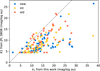 |
Fig. 16 Comparison of brightening slope K1 from JPL SBDB with k1 derived in this paper. Both axes are in units of mag/log(au), and a dashed gray line indicates K1 = k1. |
4.5 Implications for upcoming surveys and missions
This work was partially motivated by the upcoming LSST survey and Comet Interceptor (CI) mission. Developing CI without a predefined target presents clear challenges, making it essential to establish baseline expectations for potential targets. The target will likely be discovered by LSST, well beyond Jupiter (Inno et al. 2025), and its brightening will be covered in great detail, albeit too late to influence most mission parameters.
This paper scrutinizes long-standing assertions about LPC behavior using a large number of available measurements. Some of our findings are promising, particularly the evidence that new comets tend to exhibit consistent behavior. For instance, Figure 14 suggests that new comets discovered beyond Jupiter’s orbit brighten in a relatively predictable manner compared to returning comets. Furthermore, if the typical rate of brightening of new comets continues to increase beyond the heliocentric distances probed by Figure 7, this may indicate that most new comets come from the most distant parts of the Oort cloud (a > 20 000 au) have not undergone significant processing and fading before reaching a near-Earth perihelion (Kaib 2022).
Table 10 and Figure 14 can be used to convert the total magnitude of a comet discovered beyond Jupiter to an approximated, empirical probability for its total magnitude at 1 au. For instance, dynamically new comet C/2021 T4 was tracked photometrically from r = 6.9 au, inbound toward perihelion near r = 1.5 au, as part of the LOOK survey (Holt et al. 2024). Based on the initial heliocentric magnitude, mhelio ≈ 17.5 mag, we would expect a median brightening of Δm ≈ 5.2 mag (and 50% chance of 4.8 < Δm < 6.0 mag) upon reaching perihelion. According to the LOOK photometry, it reached mhelio ≈ 13 mag, so it brightened by 4.5 magnitudes, only slightly below the statistical prediction. No other comet in the LOOK survey has observations from beyond 5 au to near 1 au. However, C/2022 E3 (intermediate) is observed to brighten from approximately 14 mag at 4 au to 11.5 mag at 2 au (brightening of 2.5 mag) and to 10 mag at 1 au (brightening of 4 mag), while Table 10 would predict median brightening of 2.55 and 5.8 mag in the same heliocentric ranges. Comet C/2021 O3 (new) brightened 1.4 magnitudes (from 17.5 to 16.1 mag) between 4.2 and 3 au, compared to the a brightening of 1.62 mag between 4 and 3 au predicted by Table 10.
5 Conclusions
In this study, we investigated the secular brightening behavior of 272 long-period comets by analyzing a large sample of highly heterogeneous photometric observations. Using a robust selection process, we derived local and global brightening parameters, accounting for potential biases in the data. We examined how brightening rates vary with heliocentric distance and explored differences between dynamically new, intermediate, and old LPCs, and between pre- and post-perihelion observations. Below, we summarize the key conclusions of this work.
We find that dynamically new comets brighten more slowly than old comets. The difference in brightening rate is notable within 3 au from the Sun but becomes negligible beyond that distance;
For new comets, the brightening rate varies with heliocentric distance becoming shallower as they approach the Sun: beyond 3 au they brighten at a rate around 12.8 mag per log au, whereas within 3 au from the Sun, their brightening rate decreases to below 7 mag per log au. Dynamically old comets brighten about 14 mag per log au in the entire range within 6 au of the Sun, displaying more scatter in their brightening behavior;
Post-perihelion fading slopes are consistent across Oort groups, with little variation between new and returning comets;
Dynamically new comets exhibit more uniform photometric behavior compared to returning comets, with a tighter correlation between brightening parameters k1 and m1;
Dynamically new comets are intrinsically brighter than old comets, possibly due to larger nuclei or higher activity levels.
These findings shed light on how comet brightening evolves with heliocentric distance and dynamical history, and help characterize systematic differences between new and returning comets. Upcoming surveys with better characterized data will be key to further constraining the physical properties of dynamically new comets.
Data availability
The full table of observations used in the paper, the table of processed strands and global curves and their properties, as well as the table of rejected strands and global curves are all available online here.
Acknowledgements
We thank David Jewitt for comments on the manuscript, and the referee for a detailed review which resulted in a paper with more robust statistics. PL acknowledges funding by Fundação para a Ciência e a Tecnologia (FCT) through the research grants UIDB/04434/2020 (DOI: 10.54499/UIDB/04434/2020) and UIDP/04434/2020 (DOI: 10.54499/UIDP/04434/2020). AGL was supported by CNES (mission Comet Interceptor) and funding from the European Research Council (ERC) under the European Union’s Horizon 2020 research and innovation programme (Grant Agreement No 802699). RK would like to acknowledge the support from “L’Oreal UNESCO For Women in Science” National program for Bulgaria. RK acknowledges partial support by grant: KII-06-H88/5 “Physical properties and chemical composition of asteroids and comets – a key to increasing our knowledge of the Solar System origin and evolution” by the Bulgarian National Science Fund. LI acknowledges support by the Italian Space Agency (ASI) within the ASI-INAF agreements I/024/12/0 and 2020-4-HH.0.
Appendix A Sample of observations
Figure A.1 shows a larger sample of curves. For the full dataset of observations follow this online link.
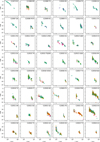 |
Fig. A.1 Larger subset of observations grouped by comet. Colors correspond to different observatories and symbols to different photometric bands. |
References
- A’Hearn, M. F., Millis, R. C., Schleicher, D. O., Osip, D. J., & Birch, P. V. 1995, Icarus, 118, 223 [Google Scholar]
- Bauer, J. M., Grav, T., Fernández, Y. R., et al. 2017, AJ, 154, 53 [Google Scholar]
- Betzler, A. S., Diepvens, A., & de Sousa, O. F. 2023, MNRAS, 526, 246 [Google Scholar]
- Bouziani, N., & Jewitt, D. 2022, ApJ, 924, 37 [NASA ADS] [CrossRef] [Google Scholar]
- Dello Russo, N., Kawakita, H., Vervack, R. J., & Weaver, H. A. 2016, Icarus, 278, 301 [NASA ADS] [CrossRef] [Google Scholar]
- Delsemme, A. H. 1982, in IAU Colloq. 61: Comet Discoveries, Statistics, and Observational Selection, ed. L. L. Wilkening, 85 [Google Scholar]
- Duncan, M., Quinn, T., & Tremaine, S. 1987, AJ, 94, 1330 [Google Scholar]
- Fernández, J. A., Tancredi, G., Rickman, H., & Licandro, J. 1999, A&A, 352, 327 [NASA ADS] [Google Scholar]
- Francis, P. J. 2005, ApJ, 635, 1348 [NASA ADS] [CrossRef] [Google Scholar]
- Fulle, M., Blum, J., & Rotundi, A. 2020, A&A, 636, L3 [NASA ADS] [CrossRef] [EDP Sciences] [Google Scholar]
- Ginsburg, A., Sipőcz, B. M., Brasseur, C. E., et al. 2019, AJ, 157, 98 [Google Scholar]
- Gkotsinas, A., Nesvorný, D., Guilbert-Lepoutre, A., Raymond, S. N., & Kaib, N. 2024, Planet. Sci. J., 5, 243 [Google Scholar]
- Green, D. W. E. 1995, Int. Comet Q., 17, 168 [Google Scholar]
- Harrington Pinto, O., Womack, M., Fernandez, Y., & Bauer, J. 2022, Planet. Sci. J., 3, 247 [NASA ADS] [CrossRef] [Google Scholar]
- Heisler, J., & Tremaine, S. 1986, Icarus, 65, 13 [CrossRef] [Google Scholar]
- Heisler, J., Tremaine, S., & Alcock, C. 1987, Icarus, 70, 269 [Google Scholar]
- Higuchi, A., & Kokubo, E. 2015, AJ, 150, 26 [Google Scholar]
- Higuchi, A., Kokubo, E., Kinoshita, H., & Mukai, T. 2007, AJ, 134, 1693 [NASA ADS] [CrossRef] [Google Scholar]
- Hodapp, K. W., Kaiser, N., Aussel, H., et al. 2004, Astron. Nachr., 325, 636 [Google Scholar]
- Holt, C. E., Knight, M. M., Kelley, M. S. P., et al. 2024, Planet. Sci. J., 5, 273 [Google Scholar]
- Huber, P., Wiley, J., & InterScience, W. 1981, Robust Statistics (New York: Wiley) [CrossRef] [Google Scholar]
- Hughes, D. W. 1988, MNRAS, 234, 173 [Google Scholar]
- Hughes, D. W., McBride, N., Boswell, J., & Jalowiczor, P. 1993, MNRAS, 263, 247 [Google Scholar]
- Inno, L., Scuderi, M., Bertini, I., et al. 2025, Icarus, 429, 116443 [Google Scholar]
- Ivezić, Ž., Kahn, S. M., Tyson, J. A., et al. 2019, ApJ, 873, 111 [Google Scholar]
- Jewitt, D. 1991, in Astrophysics and Space Science Library, 167, IAU Colloq. 116: Comets in the post-Halley era, eds. J. Newburn, R. L. M. Neugebauer, & J. Rahe, 19 [Google Scholar]
- Jewitt, D. 2022, AJ, 164, 158 [Google Scholar]
- Jewitt, D., Agarwal, J., Hui, M.-T., et al. 2019, AJ, 157, 65 [NASA ADS] [CrossRef] [Google Scholar]
- Jewitt, D., Kim, Y., Mutchler, M., et al. 2021, AJ, 161, 188 [NASA ADS] [CrossRef] [Google Scholar]
- Jones, G. H., Snodgrass, C., Tubiana, C., et al. 2024, Space Sci. Rev., 220, 9 [NASA ADS] [CrossRef] [Google Scholar]
- Kaib, N. A. 2022, Sci. Adv., 8, eabm9130 [Google Scholar]
- Kaib, N. A., & Quinn, T. 2009, Science, 325, 1234 [NASA ADS] [CrossRef] [Google Scholar]
- Keller, H. U., & Kührt, E. 2020, Space Sci. Rev., 216, 14 [Google Scholar]
- Królikowska, M., & Dybczyński, P. A. 2020, A&A, 640, A97 [NASA ADS] [CrossRef] [EDP Sciences] [Google Scholar]
- Larson, S., Beshore, E., Hill, R., et al. 2003, in AAS/Division for Planetary Sciences Meeting Abstracts, 35, 36.04 [Google Scholar]
- Maggiolo, R., Gronoff, G., Cessateur, G., et al. 2020, ApJ, 901, 136 [NASA ADS] [CrossRef] [Google Scholar]
- Mainzer, A., Bauer, J., Grav, T., et al. 2011, ApJ, 731, 53 [Google Scholar]
- Malamud, U., Landeck, W. A., Bischoff, D., et al. 2022, MNRAS, 514, 3366 [NASA ADS] [CrossRef] [Google Scholar]
- Marshall, D., Rezac, L., Hartogh, P., Zhao, Y., & Attree, N. 2019, A&A, 623, A120 [NASA ADS] [CrossRef] [EDP Sciences] [Google Scholar]
- Mazzotta Epifani, E., Perna, D., Di Fabrizio, L., et al. 2014, A&A, 561, A6 [NASA ADS] [CrossRef] [EDP Sciences] [Google Scholar]
- Meech, K. J., & Svoren, J. 2004, in Comets II, eds. Festou, M. C., Keller, H. U., & H. A. Weaver (University of Arizona Press), 317 [Google Scholar]
- Meisel, D. D. 1970, AJ, 75, 252 [Google Scholar]
- Meisel, D. D., & Morris, C. S. 1976, in NASA Special Publication, 393, eds. B. Donn, M. Mumma, W. Jackson, M. A’Hearn, & R. S. Harrington (NASA), 410 [Google Scholar]
- Meisel, D. M., & Morris, C. S. 1982, in IAU Colloq. 61: Comet Discoveries, Statistics, and Observational Selection, ed. L. L. Wilkening, 413 [Google Scholar]
- Oort, J. H. 1950, Bull. Astron. Inst. Netherlands, 11, 91 [NASA ADS] [Google Scholar]
- Oort, J. H., & Schmidt, M. 1951, Bull. Astron. Inst. Netherlands, 11, 259 [Google Scholar]
- Pfalzner, S., Govind, A., & Portegies Zwart, S. 2024, Nat. Astron., 8, 1380 [NASA ADS] [CrossRef] [Google Scholar]
- Robinson, J. E., Malamud, U., Opitom, C., Perets, H., & Blum, J. 2024, MNRAS, 531, 859 [Google Scholar]
- Sárneczky, K., Szabó, G. M., Csák, B., et al. 2016, AJ, 152, 220 [Google Scholar]
- Smith, K. W., Smartt, S. J., Young, D. R., et al. 2020, PASP, 132, 085002 [Google Scholar]
- Snodgrass, C., & Holt, C. 2024, in European Planetary Science Congress, EPSC2024-324 [Google Scholar]
- Sosa, A., & Fernández, J. A. 2011, MNRAS, 416, 767 [NASA ADS] [Google Scholar]
- Stokes, G. H., Evans, J. B., Viggh, H. E. M., Shelly, F. C., & Pearce, E. C. 2000, Icarus, 148, 21 [NASA ADS] [CrossRef] [Google Scholar]
- van Woerkom, A. J. J. 1948, Bull. Astron. Inst. Netherlands, 10, 445 [Google Scholar]
- Weissman, P. R. 1980, A&A, 85, 191 [NASA ADS] [Google Scholar]
- Whipple, F. L. 1978, Moon Planets, 18, 343 [Google Scholar]
- Whipple, F. L. 1992, in Asteroids, Comets, Meteors 1991, eds. A. W. Harris, & E. Bowell, 633 [Google Scholar]
- Wiegert, P., & Tremaine, S. 1999, Icarus, 137, 84 [Google Scholar]
- Yang, B., Jewitt, D., Zhao, Y., et al. 2021, ApJ, 914, L17 [NASA ADS] [CrossRef] [Google Scholar]
We renamed Oort’s “fairly new” category as intermediate.
As an example, of the 516 LPCs in the Nakano Note, only 26 are classified differently using MPC orbits, 19 moving from intermediate to new, 5 moving the other way around, and 2 moving from intermediate to old. These differences have no impact on the conclusions presented in this paper.
RLM works by iteratively weighting down outliers following a specific function. We use Python’s statsmodels implementation of RLM with the default outlier weighting function HuberT (Huber et al. 1981).
Implemented using Python’s scipy.stats.ks_2samp function ks_2samp.
This information was provided by JPL SSD support staff at our request, after failing to find details in the literature or on the SSD website.
All Tables
Bootstrap comparisons of strand and global curve parameters across Oort groups and orbital arcs.
Magnitude brightening distribution as a function of heliocentric distance organized by Oort group.
All Figures
|
Fig. 1 Small subset of observations grouped by comet. Colors correspond to different observatories and symbols to different photometric bands. A larger sample appears in Appendix A. |
| In the text | |
|
Fig. 2 Strands (top panel array) and global curve (bottom panel) for comet C/2019 U6. Top array panels are labeled by MPC observatory code (E89=Geyserland, F51=Pan-STARRS 1, Q38=Lake Boga, T05=ATLAS-HKO, T08=ATLS-MLO, W88=Slooh). Top-panel legends indicate strand filter and whether strands are valid or invalid, the latter indicated as the reason for rejection. Global curve legend indicates filter (same symbols as top array panels), for comparison. We note that the global curve may include points from invalid strands, e.g., green diamonds in top sub-panel F51, which means they were not useful to assess local slope, but are useful to assess the global behavior. |
| In the text | |
|
Fig. 3 Distribution of 1/a0 for strands (multiple per comet) and global curves (one or two per comet). Oort group ranges are identified. |
| In the text | |
|
Fig. 4 Distribution of strands into comets and over heliocentric distance. Pre-perihelion strand midpoints (vertical axis) are plotted as open circles for each comet (horizontal axis) in the original sample (644 strands for 141 comets). Horizontal dotted lines mark heliocentric bin boundaries. Numbers of strands and comets in each bin in the original sample are shown separated by a slash to the right of the Figure. A debiased strand sample (see text for details) is overplotted as red dots. |
| In the text | |
|
Fig. 5 Cumulative probability distributions (top) and histograms (bottom) of the kr brightening parameter for pre-perihelion strands, by Oort group. Shown are averages of Ni = 100 debiased strand sample distributions (see text for details). Histogram counts were rescaled so that they add up to the actual number of pre-perihelion strands measured. |
| In the text | |
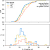 |
Fig. 6 Same as Figure 5 but for the k1 brightening parameter fit to preperihelion global curves. |
| In the text | |
|
Fig. 7 Brightening slope of strands as a function of heliocentric distance. A range of distance boundaries, shown as vertical dotted lines labeled by distance, separate strands into interior and exterior to the boundary. Two horizontal lines extending from each boundary to the left and to the right connect to boxes that correspond to interior and exterior strands, respectively. The x coordinate of each box is the median of the midpoint in log r of the strands. The y extent of each box contains the IQR of the kr distribution. Inside each box, a horizontal line marks the median and a star symbol indicates the mean of the kr distribution. |
| In the text | |
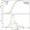 |
Fig. 8 Same as Figure 5 but for the kr fading parameter corresponding to post-perihelion strands. |
| In the text | |
|
Fig. 9 Same as Figure 6 but for the k1 fading parameter corresponding to post-perihelion global curves. |
| In the text | |
|
Fig. 10 Difference between brightening and fading slopes of global curves. A robust linear model fit of the form Δk1 = −0.65(k1 − 11.6) is shown (adjusted R2 = 0.27). |
| In the text | |
|
Fig. 11 Median mr for strands as a function of heliocentric distance and Oort group (shown to the right of the vertical dashed line). Strands are binned in equal-sized rmin bins (linear r), and the median mr and median absolute deviation are plotted as points and error bars, respectively. Bin centers coincide with the x-axis location of the “int.” symbols and the “new” and “old” symbols where horizontally nudged for clarity. To the left of the vertical dashed line are the m1 distribution median plus or minus the mean absolute deviation for global curves. |
| In the text | |
|
Fig. 12 Empirical cumulative probability distribution of the m1 parameter for pre-perihelion global curves organized by Oort group. |
| In the text | |
|
Fig. 13 Relation between m1 and k1 for pre-perihelion global curves, color-coded by Oort group. Points correspond to individual comets. Black lines are RLM fits to each Oort group. The respective fit coefficients of determination are |
| In the text | |
|
Fig. 14 Average relative magnitude brightening per Oort group. Median magnitudes are calculated for each comet in heliocentric distance bins, grouped by Oort classification and averaged. See text for details. Shading connecting points and 1σ standard error bars are added to guide the eye. Bin centers coincide with the x-axis location of the “int.” symbols and the “new” and “old” symbols where horizontally nudged for clarity. |
| In the text | |
|
Fig. 15 Relation between the brightening slope k1 of global curves and CO/H2O abundance in the coma. |
| In the text | |
|
Fig. 16 Comparison of brightening slope K1 from JPL SBDB with k1 derived in this paper. Both axes are in units of mag/log(au), and a dashed gray line indicates K1 = k1. |
| In the text | |
|
Fig. A.1 Larger subset of observations grouped by comet. Colors correspond to different observatories and symbols to different photometric bands. |
| In the text | |
Current usage metrics show cumulative count of Article Views (full-text article views including HTML views, PDF and ePub downloads, according to the available data) and Abstracts Views on Vision4Press platform.
Data correspond to usage on the plateform after 2015. The current usage metrics is available 48-96 hours after online publication and is updated daily on week days.
Initial download of the metrics may take a while.