| Issue |
A&A
Volume 697, May 2025
|
|
|---|---|---|
| Article Number | A220 | |
| Number of page(s) | 15 | |
| Section | Stellar structure and evolution | |
| DOI | https://doi.org/10.1051/0004-6361/202451879 | |
| Published online | 20 May 2025 | |
Feasibility study of a dark matter admixed neutron star based on recent observational constraints
1
Department of Physics, BITS-Pilani, K. K. Birla Goa Campus, Goa 403726, India
2
CFisUC, Department of Physics, University of Coimbra, P-3004 – 516 Coimbra, Portugal
3
Department of Physics, Birla Institute of Technology and Science Pilani, Pilani Campus, Pilani, Rajasthan 333031, India
4
Department of Sciences, Amrita School of Physical Sciences, Amrita Vishwa Vidyapeetham, Coimbatore 641112, India
⋆ Corresponding author: tuhin.malik@uc.pt
Received:
13
August
2024
Accepted:
2
March
2025
Context. The equation of state (EOS) for neutron stars is modeled using the relativistic mean field (RMF) approach with a mesonic nonlinear (NL) interaction, a modified sigma potential (NL–σ cut) that mimics the effect of an exclusion volume or the onset of a quarkyonic phase, and influences of dark matter in the NL (NL DM). Experimental constraints on the general properties of finite nuclei and heavy ion collisions, as well as astrophysical observations of neutron star radii and tidal deformation are taken into account.
Aims. We evaluate the plausibility and implications of each scenario by exploring how modifications to the RMF model, including the NL–σ cut and dark matter influences, affect the neutron star EOS. Additionally, the study examines the tension between the PREX-II experimental data and other constraints, aiming to identify which model is able to optimally reconcile the available experimental and observational evidence.
Methods. A Bayesian analysis framework was employed to systematically compare the different EOS scenarios. This approach integrates constraints from nuclear experiments (finite nuclei properties and heavy ion collisions) and astrophysical observations (neutron star radii, tidal deformation, and PSR J0437–4715 measurements) to rigorously assess the viability of each model.
Results. The analysis shows that including the PREX–II data renders all models less favorable, indicating significant tension with the other constraints and incompatibility with chiral effective field theory calculations of pure neutron matter. When excluding PREX–II, the NL–σ cut model emerges with the highest Bayes evidence, favoring a stiffening of the EOS at high densities, whereas the model incorporating a dark matter component is the least favorable. Furthermore, new PSR J0437–4715 measurements lead to an approximate 0.2 km reduction in the 90% confidence interval upper boundary for neutron star radii, along with a notable decrease in Bayesian evidence, suggesting potential conflicts with prior data and/or the need for more adaptable models.
Key words: stars: neutron / stars: oscillations / dark matter
© The Authors 2025
 Open Access article, published by EDP Sciences, under the terms of the Creative Commons Attribution License (https://creativecommons.org/licenses/by/4.0), which permits unrestricted use, distribution, and reproduction in any medium, provided the original work is properly cited.
This article is published in open access under the Subscribe to Open model. Subscribe to A&A to support open access publication.
1. Introduction
The equation of state (EOS) of neutron stars is pivotal in determining their internal structure and observable characteristics, such as mass and radius. Various microscopic many-body approaches and phenomenological models have been employed to reconstruct the EOS, taking into account the interactions of nucleons, hyperons, and other exotic particles Gal et al. (2016), Curceanu et al. (2019), Tolos & Fabbietti (2020). The EOS models are validated against both terrestrial laboratory data and astrophysical observations Malik & Providência (2022), Dutra et al. (2014), Oertel et al. (2017), Burgio et al. (2021). Furthermore, the detection of gravitational waves from neutron star mergers provides additional constraints, with postmerger emissions offering insights into the EOS by correlating specific spectral features with the star’s compactness Takami et al. (2014). Recent studies have shown that the onset of phase transition from hadronic matter to quark matter can significantly affect the dynamics and gravitational wave signals of binary neutron star mergers Weih et al. (2020), Haque et al. (2023). One area of research that has recently attracted considerable interest is altered gravity theories, with the study of neutron stars within the framework of modified gravity theories being a lively field of research, offering an opportunity to compare the predictions of these theories with observational data (Nobleson et al. 2023; Alam et al. 2024; Cooney et al. 2010; Yazadjiev et al. 2018). The combined efforts from both theoretical and observational studies are essential for enhancing our understanding of the extreme conditions within neutron stars. Recent studies have extended this understanding by incorporating the effects of dark matter (DM) within neutron stars (Ellis et al. 2018; Das et al. 2019, 2022; Nelson et al. 2019; Karkevandi et al. 2022; Lenzi et al. 2023; Giangrandi et al. 2023; Rutherford et al. 2023; Routaray et al. 2023; Shakeri & Karkevandi 2024; Singh et al. 2023; Thakur et al. 2024a; Sagun et al. 2023; Diedrichs et al. 2023; Cronin et al. 2023; Flores et al. 2024; Scordino & Bombaci 2025; Barbat et al. 2024). Dark matter, interacting with neutrons through mechanisms such as Higgs boson exchange, significantly alters the EOS, potentially leading to observable changes in neutron star characteristics. For instance, DM can affect the mass-to-radius relation (Das et al. 2020, 2021a,b; Sen & Guha 2021, 2022; Guha & Sen 2021; Lourenço et al. 2022; Shirke et al. 2023, 2024; Panotopoulos & Lopes 2017) and the cooling rates of neutron stars (Kouvaris 2008; Giangrandi et al. 2024). Studies show that neutron stars containing a mix of baryonic and dark matter might exhibit different mass-radius relations, compared to those composed solely of neutron matter, influencing gravitational redshift and potentially explaining observations that are inconsistent with typical neutron stars Rezaei (2017).
Numerous candidates for dark matter particles, including bosonic dark matter, axions, sterile neutrinos, and various WIMPs, have been discussed (Silk et al. 2010; Bauer & Plehn 2019; Calmet & Kuipers 2021). The nature of dark matter and its properties, such as self-interaction and coupling with standard model particles, have been explored for their impact on neutron star dynamics (Ellis et al. 2018; Panotopoulos & Lopes 2017; Diedrichs et al. 2023; Leung et al. 2022; Narain et al. 2006). Two commonly researched methods for examining neutron stars mixed with dark matter can be found in the current literature. One approach considers non-gravitational interactions, using such mechanisms as the Higgs portal (Dutra et al. 2022; Lenzi et al. 2023; Hong & Ren 2024; Das et al. 2019, 2020; Flores et al. 2024; Sen & Guha 2021). The other approach considers only gravitational interactions, treated as a two-fluid system (Collier et al. 2022; Miao et al. 2022; Emma et al. 2022; Hong & Ren 2024; Karkevandi et al. 2022; Rüter et al. 2023; Liu et al. 2023; Ivanytskyi et al. 2020; Buras-Stubbs & Lopes 2024; Rutherford et al. 2023). Another method involves the neutron decay into dark matter particles that accounts for the neutron decay anomaly (Husain et al. 2022; Bastero-Gil et al. 2024; Baym et al. 2018; Shirke et al. 2023, 2024; Motta et al. 2018). This can be addressed using either a single-fluid method or a two-fluid method. Discrepancies in neutron decay lifetimes measured via bottle and beam experiments suggest a greater number of decayed neutrons than produced protons, possibly due to decay into nearly degenerate dark fermions.
To understand the mixed dark matter scenario in neutron stars (NSs), knowledge of the equation of state (EOS) for both baryonic and dark matter is crucial. The dense matter EOS is based on a microscopic approach, which allows for a determination of the NS composition and can be described by relativistic and nonrelativistic models. Nonrelativistic models describe nucleons within finite nuclei well, but fail with infinite dense nuclear matter giving rise to non-causal EOS. Relativistic mean-field (RMF) models, suitable for describing both finite nuclei and high-density matter in NSs, incorporate many-body interactions via mesons (σ, ω, ρ). Two main RMF approaches describe nuclear properties: nonlinear meson terms in the Lagrangian density (Boguta & Bodmer 1977; Mueller & Serot 1996; Steiner et al. 2005; Todd-Rutel & Piekarewicz 2005) and density-dependent coupling parameters (Typel & Wolter 1999; Typel et al. 2010; Lalazissis et al. 2005). A different, more general approach is an agnostic description of the EOS that can be parametric or non-parametric. These approaches include piecewise polytropic interpolation, speed of sound interpolation, spectral interpolation, Taylor expansion, and Gaussian processes (Lindblom & Indik 2012; Kurkela et al. 2014; Most et al. 2018; Lope Oter et al. 2019; Annala et al. 2020, 2022; Landry et al. 2020; Essick et al. 2020), among others. Possible EOSs are determined by imposing low and high-density theoretical calculations constraints (Hebeler et al. 2013; Drischler et al. 2016; Kurkela et al. 2010) and astrophysical constraints (Abbott et al. 2018; Fonseca et al. 2021; Riley et al. 2019, 2021; Miller et al. 2019, 2021). These approaches fail to predict the composition of NS.
Our study explores the non-linear model within the RMF framework. This choice has an associated energy density functional that is not completely general, but has already been shown to describe both nuclear and neutron star properties quite successfully. This can be seen from prior studies (Sugahara & Toki 1994; Lalazissis et al. 1997; Horowitz & Piekarewicz 2001; Todd-Rutel & Piekarewicz 2005; Providência et al. 2014; Chen et al. 2014; Tolos et al. 2017). In these studies, different parameterizations of the model constrained by nuclear and neutron star properties are proposed. The mass-radius region spanned by the model with some minimal nuclear matter properties and NS observational constraints obtained in Malik et al. (2023) is broader than the corresponding region obtained from a model with built-in chiral symmetry, as shown in Malik et al. (2024). A broader mass-radius region could have been spanned if an RMF with density dependent coupling constants had been used, as shown in Providência et al. (2023). However, in the present study, we have chosen to use a more controllable functional, which allows for an EOS with a speed-of-sound square that goes to 1/3 at high densities.
While the EOS of nuclear matter is quite well constrained by experimental measurements close to the saturation density and below, this is not the case for the high-density EOS. The observation of two solar-mass NSs indicates that the EOS needs to be stiff at high densities. In order to account for the stiffening of the EOS above approximately two times saturation density, the σ-cut potential approach was proposed in Maslov et al. (2015). Within this description, a sharp increase of the mean field self-interaction potential is imposed above the nuclear saturation density (ρ0), which effectively stiffens the EOS without affecting nuclear matter properties near ρ0 (Ma et al. 2022). Few studies on the σ-cut scheme focus on EOS stiffness implications, including kaon condensation, hyperons in neutron stars (Ma et al. 2022), stellar properties, nuclear matter constraints (Dutra et al. 2016; Pais & Providência 2016), strangeness neutron stars within RMF (Zhang et al. 2018), NICER data analysis (Kolomeitsev & Voskresensky 2024), and effects on pure nucleonic and hyperonic-rich NS matter (Thakur et al. 2024b). The stiffening obtained with the introduction of the σ cut potential can be seen as the inclusion of an exclusion volume effect (Typel 2016) or even as a mimicking of the onset of another baryonic phase, such as the quarkyonic phase (McLerran & Reddy 2019). In the present study, this is the mechanism used to impose a stiffening of the EOS at high densities.
As upcoming observational data become increasingly refined, we are motivated to conduct a systematic study of the interior structure of neutron stars under three distinct scenarios. Here, we considered neutron stars comprising only nucleonic degrees of freedom within the framework of the non-linear (NL) model (NL scenario). Second, we modified the NL model to include a σ-cut potential (NL-σ cut scenario) and stiffen the EOS above ∼2ρ0. Third, we investigated neutron stars that contain an admixture of dark matter, specifically focusing on fermionic dark matter for simplicity (NL-DM scenario). Previous studies have indicated that the presence of dark matter tends to reduce both the mass and radius of neutron stars. Conversely, incorporating a σ-cut potential has been shown to increase these parameters. Given these contrasting effects, our goal has been to calculate the Bayesian evidence for each of these three scenarios, thereby determining which model is most consistent with the latest observational data. By systematically evaluating these models, we aim to rank them based on their alignment with recent observations, providing a clearer understanding of the interior structure of neutron stars and the potential influence of dark matter and modified nucleonic interaction.
We performed a detailed statistical analysis using the current astrophysical observational data on NS properties within the Bayesian inference framework to explore the potential existence of DM in NS. Both baryonic (visible) matter and dark matter were considered within the RMF framework. The EOSs were developed using empirical constraints based on experimental data regarding the properties of finite nuclei and observations from astrophysics. The nuclear matter properties taken into account include the pressure of symmetric nuclear matter (PSNM), the pressure resulting from symmetry energy (Psym), and the symmetry energy itself (esym). These properties were empirically constrained across various densities using experimental data on the bulk characteristics of finite nuclei, such as nuclear masses, neutron skin thickness in 208Pb, dipole polarizability, isobaric analog states, and heavy ion collision (HIC) data covering the density range from 0.03 to 0.32 fm−3. Additionally, astrophysical data utilized here include the mass-radius posterior distributions for PSR J0030+0451 (Riley et al. 2019; Miller et al. 2019) and PSR J0740+6620 (Miller et al. 2021; Riley et al. 2021), as well as the posterior distribution for dimensionless tidal deformability for components of binary neutron stars from the GW170817 event.
We investigated which of these three scenarios, NL, NL-σ cut, or NL-DM, are better aligned with recent observational data on NS. In addition, we analyzed the impact of PREX-II experimental data in the nuclear scenarios in detail by performing a Bayesian inference, with and without this constraint; this is because PREX-II data often contradict various other nuclear data reported in the literature (Imam et al. 2024). With the present study, we hope to provide further evidence in favor or against the three scenarios and the compatibility of PREX II data with other nuclear constraints.
The structure of this paper is as follows. The results are discussed in Sect. 2. Our conclusions and main insights of the study are presented in Sect. 3. Lastly, Appendix A covers the theoretical framework used in this study.
2. Results
We analyzed various EOS and neutron star properties, considering the three different scenarios defined before: i) neutron stars (NSs) with only nucleonic degrees of freedom, modeled using the relativistic mean field (RMF) approach with mesonic nonlinear interaction (NL); ii) NS with nucleonic degrees of freedom in the RMF model, but with a modified σ potential (NL-σ cut); and iii) NS with admixed dark matter, where the nucleonic matter is modeled with NL and the dark matter is produced by the neutron decay channel as mentioned in Fornal & Grinstein (2018) (NL-DM). In addition to these three scenarios, we also discuss the effect of including the experimental PREX-II data and the observational data obtained for the recent pulsar PSR J0437-4715 within the Bayesian inference framework.
2.1. Effect of the NL-σ cut potential and PREX-II data
In this subsection, we discuss the effect of including the modified σ potential in the RMF description (NL versus NL σ-cut) and of introducing the PREX-II constraints in the Bayesian inference. We first analyzed the effect on the EOS by comparing the speed of sound squared, cs2, obtained in both descriptions and shown in Fig. 1 (left panel) and the parameter derived from the trace anomaly, dc, introduced in Annala et al. (2023), as shown in Fig. 1 (right panel).
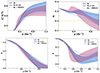 |
Fig. 1. 90% confidence intervals for cs2, (top left) |

The left panel of Fig. 1 presents the 90% confidence intervals (CI) for cs2 as a function of baryon density, (ρ), while comparing NL with and without the PREX-II constraint, alongside results from the NL-σ cut. The PREX-II data have an insignificant effect on cs2, since these data primarily affect the density dependence of the symmetry energy, and the squared speed of sound is largely determined by the symmetric nuclear matter EOS. Between the two scenarios, NL and NL-σ cut, we conclude that the modifications to the σ potential in the NL-σ cut result in a stiffer cs2 at low densities below 0.5 fm−3, becoming softer at higher densities. This occurs because, in the NL-σ cut model, the σ field saturates due to a very stiff σ potential and the effective mass stays at a constant value that may take values above 0.5 mN. As discussed in Maslov et al. (2015), the pressure increases and as a consequence larger NS maximum masses are reached and medium and high mass NS have larger radii. In order to satisfy the observational constraints, it is necessary to have a stronger ω4 term at high densities to mitigate the effect of the repulsive ω potential when it becomes dominant. Indeed, as can be seen from the Table 5, the median value of the ξ coupling more than doubles, increasing from 0.005 to 0.011. As discussed in Mueller & Serot (1996) (see also Malik et al. 2023), this term causes the speed of sound squared to tend towards 1/3 at high densities, and the larger the coupling the faster this limit is reached.
Another quantity that characterizes EOS is the parameter dc, introduced in Annala et al. (2023), defined as  , where
  is the renormalized trace anomaly introduced in Fujimoto et al. (2022),
  denotes the logarithmic derivative of Δ, and
  . In the conformal limit, cs2 and γ reach 1/3 and 1, respectively. It has been proposed that a value dc ≲ 0.2 suggests a proximity to the conformal limit, as both Δ and its derivative need to be small for this to hold true. Since quark matter is expected to show approximate conformal symmetry, a small value for dc could be indicative of the presence of quark matter. In Fig. 1 (right panel), we present the posterior distribution of dc as a function of density for the three cases examined: NL with and without PREX-II data, and NL-σ-cut. Notably, even when incorporating only nucleonic degrees of freedom, dc drops below 0.2 for all the three case in the density range of 0.6–0.7 fm−3. This result is aligned with findings from other nucleonic models Santos et al. (2024), Marquez et al. (2024), Malik et al. (2024). The behavior is primarily dictated by the ω4 term, as previously identified in Malik et al. (2024) and Malik et al. (2023).
The region shaded in blue illustrates the 90% confidence interval for the NL model, while the blue dashed lines denote the inclusion of NL along with PREX II. As density increases, dc initially decreases, followed by an increase, reaching a small peak around 0.5 fm−3, and subsequently exhibits a clear downward trend. Then, NL with PREX-II follows the same trend as NL, but lies slightly below it. For the NL-σ cut model, shown as the pink region, a similar decreasing trend is observed, but it peaks earlier, around 0.4 fm−3, with a more pronounced peak due to the stiffening of the σ potential. This stiffening reduces the need for the omega meson’s contribution to achieve high-mass neutron stars. As a result, the coupling constant gω is smaller in this case, while the ω4 term coupling is larger, leading to an overall softer EOS at very high densities. This effect is visible in the speed of sound squared (cs2), which rises rapidly at intermediate densities due to the sigma-cut contribution but then stabilizes or even decreases above ρ = 0.4 fm−3. The impact of this behavior on dc can be understood through Δ′. Initially, as pressure increases rapidly, P/ϵ also increases, but when the speed of sound stabilizes, P/ϵ saturates at a lower value compared to other EOS scenarios. This leads to a larger Δ′ and since the transition from stiff to soft EOS is more pronounced in the sigma-cut case, Δ′ also exhibits a significant change, producing the observed bump in dc. After this transition, the effect of Δ diminishes, and dc stabilizes. Additionally, in the conformal limit at very high densities, both Δ and Δ′ should ideally approach zero. The presence of the ω4 term in our case accelerates the approach of cs2 toward 1/3, similar to what is observed in agnostic EOS studies Annala et al. (2023). In those cases, a bump in dc emerges because the EOS must be stiff at low densities to support 2 M⊙ stars, but softer at high densities to comply with perturbative QCD constraints. Although our study does not impose pQCD constraints, the sigma-cut EOS naturally leads to a similar effect due to the role of the ω4 term. To validate this, we have plotted both Δ and Δ′ as function of baryon density in Fig. 1 (bottom panels).
Figure 2 depicts the mass-radius (M-R) and mass-tidal deformability (M-Λ) relationships of neutron stars based on the different scenarios considered above, compared with different astrophysical observational data. In the left panel results for the NL (blue), NL-σ cut (red), and the corresponding distributions when the PREX-II constraints are also included, respectively, the dashed blue and red lines, are plotted. In the right panels, the mass-tidal deformability are shown for the same scenarios. All distributions correspond to 90% confidence intervals. We compare our results with several observational constraints. In the left panel, the grey region shows constraints from the binary components of the gravitational wave event GW170817, including their 90% and 50% credible intervals (CI). Constraints from the NICER X-ray data for the millisecond pulsar PSRJ0030+0451 are depicted in cyan and yellow color, while those for the pulsar PSRJ0740+6620 are shown in orange and peru color, both representing the 1σ (68%) CI for the 2D posterior distribution in the M-R domain. The new pulsar data PSR J0437-4715 is highlighted in a lilac shade. In the right panel, the constraints obtained from GW170817 are included for the 1.36 M⊙ tidal deformability Abbott et al. (2018).
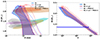 |
Fig. 2. Left: 90% credible interval (CI) region for the neutron star (NS) mass-radius posterior P(R|M) is plotted for the NL, NL-σ cut, NL + PREX-II, and NL-σ cut + PREX-II. The gray area indicates the constraints obtained from the binary components of GW170817, with their respective 90% and 50% credible intervals. Additionally, the plot includes the 1σ (68%) CI for the 2D mass-radius posterior distributions of the millisecond pulsars PSR J0030 + 0451, shown in in cyan and yellow (Riley et al. 2019; Miller et al. 2019) and PSR J0740 + 6620, shown in in orange and peru (Riley et al. 2021; Miller et al. 2021), based on NICER X-ray observations. Furthermore, we display the latest NICER measurements for the mass and radius of PSR J0437-4715 (Choudhury et al. 2024) (lilac color). Right: 90% CI region for the mass-tidal deformability posterior P(Λ|M) for the same models. The blue bars represent the tidal deformability constraints at 1.36 M⊙. |
The two posterior distributions without the PREX-II constraints diverge from each other starting around an NS mass of 1.4 M⊙. The NL-σ cut tends to shift the M-R posterior to the right, thereby increasing the radius, the larger differences occurring for the larger masses. The inclusion of the PREX-II constraints shifts the two distributions to larger radii, with the low mass NS suffering the strongest effects. This low mass effect is due to the large symmetry energy slope associated with the PREX-II constraints, a nuclear matter property that affects mostly the low mass NS: the larger the symmetry energy slope at saturation the larger the radius of a low mass NS. In Table 1, median and 90% CI of the nuclear matter and NS properties are given, and it is seen that the median of the symmetry energy slope, Lsym, 0, essentially doubles with the inclusion of the PREX-II constraints, increasing from 54 MeV to ∼105 MeV. In the right panel of Fig. 2, we confirm that the different scenarios, namely, NL and NL σ-cut without and with PREX-II, have on the tidal-deformability effects similar to the ones discussed for the radius. Specifically, NL σ-cut and the PREX-II constraints give rise to larger tidal deformabilities.
Nuclear matter and neutron star properties for different models.
It is interesting to analyze how the above scenarios agree with the ab initio chiral effective field theoretical (χEFT) calculations for pure neutron matter (PNM). In Fig. 3, we evaluate how well the computed posteriors match the χEFT calculations for PNM across all scenarios. The figure displays the posterior distributions for the NL, without and with PREX-II, and NL-σ cut without PREX-II models within the 90% confidence interval (CI) for the PNM pressure as a function of baryon density. At low densities near the saturation density, the three scenarios are indistinguishable. At larger densities, the inclusion of additional PREX-II data makes the pure neutron matter pressure significantly stiffer, pulling the posterior outside the PNM chEFT constraints. In the absence of the PREX-II constraint, the PNM pressure posterior for both NL and NL-σ cut shows a good overlap with χEFT data. It should be noted that the χEFT PNM constraints were not part of the constraints applied to the likelihood considered in this study. These data indicates the PREX-II data are in tension with χEFT constraints, contrary to all the other constraints included in our inference analysis, independently of the model considered.
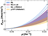 |
Fig. 3. Posterior distributions for the NL, NL-σ cut, and NL + PREX-II models within the 90% confidence interval (CI) with respect to the pressure (P) as a function of baryon density in pure neutron matter (PNM). |
The inclusion of the modified σ cut potential has a strong effect on the effective mass at high densities. Fig. 4 shows the 90% CI region for the effective mass, m*, versus baryon density, ρ, without PREX-II constraints for NL and NL-σ cut, and with PREX-II constraints for the NL model. The NL scenario shows a decreasing trend of the effective mass with density, with a minimal effect of the PREX-II data on m⋆. When the σ cut potential is applied, the effective mass stabilises above a density of 0.3 fm−3 due to the σ potential, thereby stiffening the EOS.
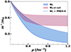 |
Fig. 4. 90% CI of effective mass (m∗) as a function of baryon density (ρ) for the NL, NL-σ-cut and NL + PREX-II models. |
In the following, we analyse the magnitude of the dR/dM derivative in order to identify possible features that distinguish the different scenarios. Figure 5 shows the dR/dM distribution for neutron stars with a mass of 1.6 M⊙ for the two models, NL and NL σ-cut, without and with the PREX-II constraints. Among the models, the NL σ-cut has the largest dR/dM slopes,  for a neutron star mass of 1.6 M⊙. The NL model has a slightly more negative slope of
  . When the additional PREX-II data are included, all slopes become more negative. The effect of the PREX-II data is to make the symmetry energy stiffer, increasing the radius for masses below 1.6 M⊙. As discussed earlier and seen in Fig. 2 left panel, the PREX-II data make the M-R distribution narrower for low mass NS, pushing the distribution to larger radii. In order to be able to still satisfy the other constraints, the MR curve slope becomes more negative.
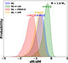 |
Fig. 5. dR/dM distribution at a neutron star mass of 1.6 M⊙ for four scenarios: NL, NL-σ cut, NL + PREX-II, and NL + DM. (The median values and related 90% confidence intervals (CI) are given on top of the respective distributions). |
2.2. Effects of dark matter
In this subsection, we discuss the implications of considering the presence of DM. The Bayesian inference was performed again, as before, considering the stellar matter described by the NL model and including the presence of DM when integrating the TOV equations. As expected (see Table 1), the nuclear matter properties are practically unaffected. The same conclusion is drawn from Fig. 6, where we compare the speed of sound squared (left panel) and the trace anomalous related parameter, dc (right panel), obtained including DM in a NL description of stellar matter NL-DM with the two previous scenarios, NL and NL-σ cut.
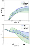 |
Fig. 6. 90% confidence intervals for cs2 (top) and dc (bottom) vs. baryon density for NL, NL-σ cut, and NL-DM models. |
Only the NS properties change in the presence of DM, as can be clearly seen in Fig. 7, where the mass-radius (left) and mass-tidal deformability (right) distributions are shown for the NL, NL-σ cut, and NL-DM scenarios. DM mainly affects medium and high mass NS, reducing the upper 90% CI limit of the radius and tidal deformability distributions and the maximum mass of the NS. Its effect is in the opposite direction to that of the modified σ potential, σ cut. These results should be reflected on the slope of the M-R curves, with NL-DM having a more negative slope than NL and than NL σ-cut, see Fig. 5.
 |
Fig. 7. 90% credible interval (CI) region for the neutron star (NS) mass-radius posterior P(R|M) is plotted for the NL, NL-σ cut, and NL-DM models. The gray area indicates the constraints obtained from the binary components of GW170817, with their respective 90% and 50% credible intervals. Additionally, the plot includes the 1σ (68%) CI for the 2D mass-radius posterior distributions of the millisecond pulsars PSR J0030 + 0451 (in cyan and yellow color) Riley et al. (2019), Miller et al. (2019) and PSR J0740 + 6620 (in orange and peru color) Riley et al. (2021), Miller et al. (2021), based on NICER X-ray observations. Furthermore, we display the latest NICER measurements for the mass and radius of PSR J0437-4715 Choudhury et al. (2024) (lilac color). Right: 90% CI region for the mass-tidal deformability posterior P(Λ|M) for the same models is presented. The blue bars represent the tidal deformability constraints at 1.36 M⊙ Abbott et al. (2018). |
In Table 1, we summarize some of the nuclear matter properties (NMP) and neutron star properties predicted by the NL, NL-σ cut, and NL-DM inference models. Some conclusions can be drawn: i) independently of the inclusion (or otherwise) of PREX-II constraints, the symmetric nuclear matter properties are only slightly affected by the inclusion of the σ cut potential and the presence of DM, in particular; in the last case, it makes it slightly harder for the EOS to compensate the effect of DM on the neutron star properties; ii) the symmetry energy and its slope at saturation do not depend on the model but the inclusion of PREX-II constraint rises the symmetry energy and its slope at saturation from 32 MeV and 54 MeV to 38 MeV and ∼105 MeV, respectively. Including PREX-II results in an increase in tidal deformability for all cases due to an increase in radius. The effect of the σ cut parameter and DM matter on the tidal deformability is clearly seen comparing Λ1.36 = 478 for the NL-σ cut model and Λ1.36 = 419 for NL-DM with Λ1.36 = 440 for the NL model. PREX-II data shifts Λ1.36 predictions to higher values: Λ1.36 = 653 for NL-PREX-II (red), Λ1.36 = 675 for NL-σ cut-PREX-II (purple), and Λ1.36 = 639 for NL-DM-PREX-II (black boundary). All models fit within or near GW170817 constraints, even when PREX-II data are included.
2.3. The Bayes factor
In the subsections above, it was shown that the effects of DM and of the σ cut potential on the NS properties as radius and tidal deformability are opposite. We aim to test which case would be favored by the current astrophysical and nuclear constraints; therefore, we calculated the Bayes factor for each inference model. The results are given in Tables 2 and 3, where the Bayes factor for each model and the Bayes factor ratios are given, respectively. Interestingly, our evidence calculations suggest that: i) the models that do not include the PREX-II constraints are favored, having systematically a higher Bayes factor; ii) considering the models with no PREX-II constraint, the model with the σ cut seems to be preferred with respect to both the NL and the NL-DM models, indicating a preference for a stiffening of the EOS at high densities. We note, however, that the evidence only indicates that there is a substantial preference of NL-σ cut with respect to NL.
Log evidence values for different models.
Log evidence differences and interpretations.
2.4. DM and σ cut potential parameters
Given that the inference analysis has been completed, we can now explore the constraints on the unknown parameter fs for the NL-σ cut and the Gχ parameter for the DM model, under the assumption of a uniform prior for both cases. The values considered for fs ranged from 0 to 1, and for Gχ, from 0 to 1000 (fm2). We define the DM self-interaction strength as
so that Gχ = 0 corresponds to the noninteracting case and increasing G enhances the repulsive self-interactions among DM particles. For a DM particle mass of m#x03C7; ≈ 938 MeV, the corresponding self-interaction cross section per unit mass is given by
Astrophysical constraints, derived from galaxy cluster observations and studies addressing the core–cusp problem, typically require
which, for m#x03C7; ≈ 1 GeV, translates to a range of approximately
Thus, by exploring a broad interval 0 ≤ Gχ ≤ 1000 fm2, we not only capture the extreme cases (from the noninteracting limit to very strong self-interactions) but also cover the region suggested by astrophysical constraints. This comprehensive range enables us to systematically assess how variations in Gχ influence neutron star observables, such as the maximum mass, tidal deformability, and thereby provides a robust framework for constraining DM properties using multimessenger astrophysical data Eckert et al. (2022), Harvey et al. (2015), Shirke et al. (2023).
In the following, we also show results including the PREX-II constraint just for reference. As expected, these constraints have essentially no effect on the parameters fs and Gχ. Figure 8 shows the probability distribution of fs for the σcut model (top panel) and of Gχ for the DM model (bottom panel) from Bayesian inference. As shown in Maslov et al. (2015), Thakur et al. (2024b), the smaller the fs, the greater the effect of the σ cut potential. It can be seen that the most likely fs compatible with the constraints lies in the range ∼0.4 − 0.6, an interval that includes fs = 0.5, the value obtained in Thakur et al. (2024b) for hyperonic stars describing two solar mass stars. The bottom panel of Fig. 8 shows that Gχ is not significantly constrained by the wide range of constraints from the nuclear and astrophysical data considered in the present study.
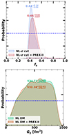 |
Fig. 8. Probability distribution of the free parameter, fs, for the σcut model (top) and Gχ for the DM model (bottom) is shown. Both panels include the distribution with and without PREX-II. The blue line indicates uniform prior. |
2.5. Impact of PSR J0437-4715
NICER’s nearest and brightest target is the 174 Hz millisecond pulsar PSR J0437-4715. Using NICER data from July 2017 to July 2021 and incorporating NICER background estimates, the latest mass-radius measurements of PSR J0437-4715 are reported in Choudhury et al. (2024). We have investigated the effect of these measurements, together with the two old NICER measurements for pulsars PSR J0030+0451 and PSR J0740+6620, on NL, NL-σ cut, and NL-DM scenarios, excluding the PREX-II constraint. Figure 9 shows the posterior distribution of neutron star mass-radius relations for the NL, NL-σ cut, and NL-DM models, respectively in panels a, b, and c, incorporating the new data from PSR J0437-4715. The inclusion of this new data particularly affects the estimated radius for neutron stars in the 1–1.5 M⊙ mass range. These new data reduces the upper limit of the 90% confidence interval by about 200 m and the lower limit by less than ∼30 m, with a consistent effect across all models. This is seen in Table 4, where the NS radius for masses of 1.2, 1.4, and 1.6 M⊙ for the three cases are given, including the new PSR constraints. We computed the Bayes evidence for each model that incorporates PSR J0437-4715 data, but excludes PREX-II and observed a decrease of ∼1 in the logarithm of the Bayes evidence in all instances (see Table 2). This suggests that the new NICER data are in conflict with the old data or that the current EOS model lacks the flexibility to simultaneously accommodate all NICER data.
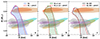 |
Fig. 9. Posterior distribution of the neutron star mass-radius P(R|M) for models (a) NL, (b) NL-σcut, and (c) NL-DM, compared with the distribution that includes the new PSR J0437-4715 NICER mass-radius measurements. The legends of NL+J0437, NL-σcut+J0437, and NL-DM+J0437 indicate the integration of PSR J0437-4715 NICER data with the previous NICER measurements. The additional constraints being compared are identical to those in Fig. 2. More information is given in the caption. |
Radius measurements with and without PSR J0437-4715 data.
Derived parameters across various posterior distributions.
3. Conclusion
In this study, we examine the equation of state (EOS) for neutron stars under three different scenarios: a purely nucleonic composition, a nucleonic composition with a σ-cut potential, and a nucleonic composition with a dark matter admixture. The effect of the σ-cut potential is to stiffen the EOS above the saturation density, with a net effect similar to the presence of a quarkyonic phase, as described in McLerran & Reddy (2019), or, alternatively, an exclusion volume Typel (2016). Using Bayesian inference and incorporating the latest constraints from nuclear physics and astrophysical observations, we were able to assess the plausibility and implications of each scenario. Our analysis shows that the inclusion of dark matter and modified potentials in the EOS significantly affects the macroscopic properties of neutron stars, such as their mass-radius and mass-tidal deformability relations.
Our results show that the inclusion of PREX-II constraints has a strong effect on several NS properties, such as the mass-radius or mass-tidal deformability curves, and, in particular, on the slope of the MR curves. The PREX-II data shift the radius of low-mass stars to very large radii on the order of 13.5–14 km. The models including PREX-II data are completely unsuccessful in reproducing the χEFT PNM pressure. In addition, the calculation of the Bayes factor has shown decisive or substantial evidence arguing against the usefulness of these models, when compared with the models without PREX-II data.
The analysis of the effect of the σ cut potential has shown that the constraints imposed in our Bayesian inference calculation favour this model, giving larger Bayes factors. The NL-σ cut model leads to a stiffening of the EOS at large densities and therefore predicts massive stars with larger radii. It also has a very pronounced effect on the speed of sound, leading to a steep increase above 0.2 fm−3 and a flattening above 0.4 fm−3. The trace anomaly related quantity is also affected, showing a clear peak for ρ ∼ 0.3 fm−3 followed by a steep decrease to values below 0.2 at 0.6 fm−3; whereas for the other models, there is no distinct peak and the values below 0.2 are only reached above 0.8 fm−3. We also analyzed the slope of the MR curve with respect to the star mass, dR/dM. The NL-σ cut model is the model that presented the largest values of dR/dM, possibly even positive, due to the presence of a stiff EOS at high densities. The calculation of the Bayes factor has also indicated that this was also the most favored model.
Finally, we examined the effect of the new PSR J0437-4715 measurements on the posterior neutron star mass-radius distribution, observing a consistent reduction of about 0.2 km in the upper bound of the 90% confidence interval across all models. The inclusion of this additional constraint was accompanied by a notable decrease in the log Bayes evidence (∼1), suggesting either a conflict with previous measurements or a need for more flexible theoretical models to accommodate the updated data.
LVK collaboration, https://dcc.ligo.org/LIGO-P1800115/public
Acknowledgments
This research is part of the Advanced Computing Project 2024.14108.CPCA.A3, with DOI identifier 10.54499/2023.14108.CPCA.A3, RNCA (Rede Nacional de Computação Avançada), funded by the FCT (Fundação para a Ciência e a Tecnologia, IPP, Portugal), and this work was produced with the support of Deucalion HPC, Portugal. The author, P.T, would like to acknowledge CFisUC, University of Coimbra, for their hospitality and local support during his visit in May – July 2023 for the purpose of conducting part of this research. The authors T.M and C.P also acknowledges the support through national funds from FCT for the projects UIDB/04564/2020 and UIDP/04564/2020, identified by DOIs 10.54499/UIDB/04564/2020 and 10.54499/UIDP/04564/2020, respectively, and for project 2022.06460.PTDC with the DOI identifier 10.54499/2022.06460.PTDC. A. D. acknowledges the New Faculty Seed Grant (NFSG), NFSG/PIL/2024/P3825, provided by the Birla Institute of Technology and Science, Pilani, India.
References
- Abbott, B. P., Abbott, R., Abbott, T. D., et al. 2018, Phys. Rev. Lett., 121, 161101 [Google Scholar]
- Abbott, B. P., Abbott, R., Abbott, T. D., et al. 2019, Phys. Rev. X, 9, 011001 [Google Scholar]
- Adhikari, D., Albataineh, H., Androic, D., et al. 2021, Phys. Rev. Lett., 126, 172502 [CrossRef] [PubMed] [Google Scholar]
- Agathos, M., Meidam, J., Del Pozzo, W., et al. 2015, Phys. Rev. D, 92, 023012 [Google Scholar]
- Alam, N., Pal, S., Rahmansyah, A., & Sulaksono, A. 2024, Phys. Rev. D, 109, 083007 [Google Scholar]
- Annala, E., Gorda, T., Kurkela, A., Nättilä, J., & Vuorinen, A. 2020, Nat. Phys., 16, 907 [NASA ADS] [CrossRef] [Google Scholar]
- Annala, E., Gorda, T., Katerini, E., et al. 2022, Phys. Rev., 12, 01058 [Google Scholar]
- Annala, E., Gorda, T., Hirvonen, J., et al. 2023, Nat. Commun., 14, 8451 [NASA ADS] [CrossRef] [Google Scholar]
- Arzumanov, S., Bondarenko, L., Chernyavsky, S., et al. 2015, Phys. Lett. B, 745, 79 [Google Scholar]
- Barbat, M. F., Schaffner-Bielich, J., & Tolos, L. 2024, Phys. Rev. D, 110, 023013 [Google Scholar]
- Bastero-Gil, M., Huertas-Roldan, T., & Santos, D. 2024, Phys. Rev. D, 110, 083003 [Google Scholar]
- Bauer, M., & Plehn, T. 2019, Yet Another Introduction to Dark Matter: The Particle Physics Approach (Springer), Lect. Notes Phys., 959 [CrossRef] [Google Scholar]
- Baym, G., Beck, D. H., Geltenbort, P., & Shelton, J. 2018, Phys. Rev. Lett., 121, 061801 [Google Scholar]
- Biswas, B., Char, P., Nandi, R., & Bose, S. 2021, Phys. Rev. D, 103, 103015 [Google Scholar]
- Boguta, J., & Bodmer, A. R. 1977, Nucl. Phys. A, 292, 413 [NASA ADS] [CrossRef] [Google Scholar]
- Brown, B. A., & Schwenk, A. 2014, Phys. Rev. C, 89, 011307 [Google Scholar]
- Buchner, J., Georgakakis, A., Nandra, K., et al. 2014, A&A, 564, A125 [NASA ADS] [CrossRef] [EDP Sciences] [Google Scholar]
- Buras-Stubbs, Z., & Lopes, I. 2024, Phys. Rev. D, 109, 043043 [Google Scholar]
- Burgio, G. F., Schulze, H. J., Vidana, I., & Wei, J. B. 2021, Prog. Part. Nucl. Phys., 120, 103879 [CrossRef] [Google Scholar]
- Byrne, J., & Dawber, P. G. 1996, EPL, 33, 187 [Google Scholar]
- Calmet, X., & Kuipers, F. 2021, Phys. Lett. B, 814, 136068 [Google Scholar]
- Chen, J.-Y., Son, D. T., Stephanov, M. A., Yee, H.-U., & Yin, Y. 2014, Phys. Rev. Lett., 113, 182302 [Google Scholar]
- Choudhury, D., Salmi, T., Vinciguerra, S., et al. 2024, ApJ, 971, L20 [NASA ADS] [CrossRef] [Google Scholar]
- Collier, M., Croon, D., & Leane, R. K. 2022, Phys. Rev. D, 106, 123027 [Google Scholar]
- Cooney, A., DeDeo, S., & Psaltis, D. 2010, Phys. Rev. D, 82, 064033 [Google Scholar]
- Cozma, M. D. 2018, Eur. Phys. J. A, 54, 40 [Google Scholar]
- Cronin, J., Zhang, X., & Kain, B. 2023, Phys. Rev. D, 108, 103016 [Google Scholar]
- Curceanu, C., Guaraldo, C., Iliescu, M., et al. 2019, Rev. Mod. Phys., 91, 025006 [CrossRef] [Google Scholar]
- Czarnecki, A., Marciano, W. J., & Sirlin, A. 2018, Phys. Rev. Lett., 120, 202002 [CrossRef] [PubMed] [Google Scholar]
- Danielewicz, P., Lacey, R., & Lynch, W. G. 2002, Science, 298, 1592 [NASA ADS] [CrossRef] [Google Scholar]
- Danielewicz, P., Singh, P., & Lee, J. 2017, Nucl. Phys. A, 958, 147 [CrossRef] [Google Scholar]
- Das, A., Malik, T., & Nayak, A. C. 2019, Phys. Rev. D, 99, 043016 [Google Scholar]
- Das, H. C., Kumar, A., Kumar, B., et al. 2020, MNRAS, 495, 4893 [Google Scholar]
- Das, H. C., Kumar, A., & Patra, S. K. 2021a, Phys. Rev. D, 104, 063028 [CrossRef] [Google Scholar]
- Das, H. C., Kumar, A., Biswal, S. K., & Patra, S. K. 2021b, Phys. Rev. D, 104, 123006 [Google Scholar]
- Das, A., Malik, T., & Nayak, A. C. 2022, Phys. Rev. D, 105, 123034 [CrossRef] [Google Scholar]
- Diedrichs, R. F., Becker, N., Jockel, C., et al. 2023, Phys. Rev. D, 108, 064009 [Google Scholar]
- Drischler, C., Hebeler, K., & Schwenk, A. 2016, Phys. Rev. C, 93, 054314 [Google Scholar]
- Dutra, M., Lourenço, O., Avancini, S. S., et al. 2014, Phys. Rev. C, 90, 055203 [Google Scholar]
- Dutra, M., Lourenço, O., & Menezes, D. P. 2016, Phys. Rev. C, 93, 025806 [NASA ADS] [CrossRef] [Google Scholar]
- Dutra, M., Lenzi, C. H., & Lourenço, O. 2022, MNRAS, 517, 4265 [Google Scholar]
- Eckert, D., Ettori, S., Robertson, A., et al. 2022, A&A, 666, A41 [NASA ADS] [CrossRef] [EDP Sciences] [Google Scholar]
- Ellis, J., Hütsi, G., Kannike, K., et al. 2018, Phys. Rev. D, 97, 123007 [CrossRef] [Google Scholar]
- Emma, M., Schianchi, F., Pannarale, F., Sagun, V., & Dietrich, T. 2022, Particles, 5, 273 [Google Scholar]
- Essick, R., Landry, P., & Holz, D. E. 2020, Phys. Rev. D, 101, 063007 [CrossRef] [Google Scholar]
- Estee, J., Lynch, W. G., Tsang, C. Y., et al. 2021, Phys. Rev. Lett., 126, 162701 [CrossRef] [PubMed] [Google Scholar]
- Fattoyev, F. J., Horowitz, C. J., Piekarewicz, J., & Shen, G. 2010, Phys. Rev. C, 82, 055803 [Google Scholar]
- Flores, C. V., Lenzi, C. H., Dutra, M., Lourenço, O., & Arbañil, J. D. V. 2024, Phys. Rev. D, 109, 083021 [Google Scholar]
- Fonseca, E., Cromartie, H. T., Pennucci, T. T., et al. 2021, ApJ, 915, L12 [NASA ADS] [CrossRef] [Google Scholar]
- Fornal, B., & Grinstein, B. 2018, Phys. Rev. Lett., 120, 191801 [Google Scholar]
- Fornal, B., & Grinstein, B. 2020, Mod. Phys. Lett. A, 35, 2030019 [Google Scholar]
- Fujimoto, Y., Fukushima, K., McLerran, L. D., & Praszalowicz, M. 2022, Phys. Rev. Lett., 129, 252702 [CrossRef] [PubMed] [Google Scholar]
- Gal, A., Hungerford, E. V., & Millener, D. J. 2016, Rev. Mod. Phys., 88, 035004 [CrossRef] [Google Scholar]
- Giangrandi, E., Sagun, V., Ivanytskyi, O., Providência, C., & Dietrich, T. 2023, ApJ, 953, 115 [Google Scholar]
- Giangrandi, E., Ávila, A., Sagun, V., Ivanytskyi, O., & Providência, C. 2024, Particles, 7, 179 [Google Scholar]
- Guha, A., & Sen, D. 2021, JCAP, 09, 027 [Google Scholar]
- Haque, S., Mallick, R., & Thakur, S. K. 2023, MNRAS, 527, 11575 [Google Scholar]
- Harvey, D., Massey, R., Kitching, T., Taylor, A., & Tittley, E. 2015, Science, 347, 1462 [Google Scholar]
- Hebeler, K., Lattimer, J. M., Pethick, C. J., & Schwenk, A. 2013, ApJ, 773, 11 [CrossRef] [Google Scholar]
- Hong, B., & Ren, Z. 2024, Phys. Rev. D, 109, 023002 [Google Scholar]
- Horowitz, C. J., & Piekarewicz, J. 2001, Phys. Rev. Lett., 86, 5647 [NASA ADS] [CrossRef] [Google Scholar]
- Husain, W., Motta, T. F., & Thomas, A. W. 2022, JCAP, 10, 028 [Google Scholar]
- Imam, S. M. A., Malik, T., Providência, C., & Agrawal, B. K. 2024, Phys. Rev. D, 109, 103025 [Google Scholar]
- Ivanytskyi, O., Sagun, V., & Lopes, I. 2020, Phys. Rev. D, 102, 063028 [Google Scholar]
- Karkevandi, D. R., Shakeri, S., Sagun, V., & Ivanytskyi, O. 2022, Phys. Rev. D, 105, 023001 [CrossRef] [Google Scholar]
- Kolomeitsev, E. E., & Voskresensky, D. N. 2024, Phys. Rev. C, 110, 025801 [Google Scholar]
- Kortelainen, M., McDonnell, J., Nazarewicz, W., et al. 2012, Phys. Rev. C, 85, 024304 [CrossRef] [Google Scholar]
- Kouvaris, C. 2008, Phys. Rev. D, 77, 023006 [Google Scholar]
- Kurkela, A., Romatschke, P., & Vuorinen, A. 2010, Phys. Rev. D, 81, 105021 [Google Scholar]
- Kurkela, A., Fraga, E. S., Schaffner-Bielich, J., & Vuorinen, A. 2014, ApJ, 789, 127 [NASA ADS] [CrossRef] [Google Scholar]
- Lalazissis, G. A., Konig, J., & Ring, P. 1997, Phys. Rev. C, 55, 540 [NASA ADS] [CrossRef] [Google Scholar]
- Lalazissis, G. A., Niksic, T., Vretenar, D., & Ring, P. 2005, Phys. Rev. C, 71, 024312 [NASA ADS] [CrossRef] [Google Scholar]
- Landry, P., Essick, R., & Chatziioannou, K. 2020, Phys. Rev. D, 101, 123007 [NASA ADS] [CrossRef] [Google Scholar]
- Le Fèvre, A., Leifels, Y., Reisdorf, W., Aichelin, J., & Hartnack, C. 2016, Nucl. Phys. A, 945, 112 [CrossRef] [Google Scholar]
- Lenzi, C. H., Dutra, M., Lourenço, O., Lopes, L. L., & Menezes, D. P. 2023, Eur. Phys. J. C, 83, 266 [Google Scholar]
- Leung, K.-L., Chu, M.-C., & Lin, L.-M. 2022, Phys. Rev. D, 105, 123010 [Google Scholar]
- Lindblom, L., & Indik, N. M. 2012, Phys. Rev. D, 86, 084003 [Google Scholar]
- Liu, H.-M., Wei, J.-B., Li, Z.-H., Burgio, G. F., & Schulze, H. J. 2023, Phys. Dark Univ., 42, 101338 [Google Scholar]
- Lope Oter, E., Windisch, A., Llanes-Estrada, F. J., & Alford, M. 2019, J. Phys. G, 46, 084001 [Google Scholar]
- Lourenço, O., Lenzi, C. H., Frederico, T., & Dutra, M. 2022, Phys. Rev. D, 106, 043010 [Google Scholar]
- Lynch, W., & Tsang, M. 2022, Phys. Lett. B, 830, 137098 [CrossRef] [Google Scholar]
- Ma, F., Guo, W., & Wu, C. 2022, Phys. Rev. C, 105, 015807 [Google Scholar]
- Malik, T., & Providência, C. 2022, Phys. Rev. D, 106, 063024 [NASA ADS] [CrossRef] [Google Scholar]
- Malik, T., Ferreira, M., Albino, M. B., & Providência, C. 2023, Phys. Rev. D, 107, 103018 [NASA ADS] [CrossRef] [Google Scholar]
- Malik, T., Dexheimer, V., & Providência, C. 2024, Phys. Rev. D, 110, 043042 [NASA ADS] [CrossRef] [Google Scholar]
- Mampe, W., Bondarenko, L. N., Morozov, V. I., Panin, Y. N., & Fomin, A. I. 1993, JETP Lett., 57, 82 [Google Scholar]
- Marquez, K. D., Malik, T., Pais, H., Menezes, D. P., & Providência, C. 2024, Phys. Rev. D, 110, 063040 [Google Scholar]
- Maslov, K. A., Kolomeitsev, E. E., & Voskresensky, D. N. 2015, Phys. Rev. C, 92, 052801 [Google Scholar]
- McLerran, L., & Reddy, S. 2019, Phys. Rev. Lett., 122, 122701 [NASA ADS] [CrossRef] [Google Scholar]
- Miao, Z., Zhu, Y., Li, A., & Huang, F. 2022, ApJ, 936, 69 [Google Scholar]
- Miller, M. C., Lamb, F. K., Dittmann, A. J., et al. 2019, ApJ, 887, L24 [Google Scholar]
- Miller, M. C., Lamb, F. K., Dittmann, A. J., et al. 2021, ApJ, 918, L28 [NASA ADS] [CrossRef] [Google Scholar]
- Morfouace, P., Tsang, C. Y., Zhang, Y., et al. 2019, Phys. Lett. B, 799, 135045 [Google Scholar]
- Most, E. R., Weih, L. R., Rezzolla, L., & Schaffner-Bielich, J. 2018, Phys. Rev. Lett., 120, 261103 [Google Scholar]
- Motta, T. F., Guichon, P. A. M., & Thomas, A. W. 2018, Int. J. Mod. Phys. A, 33, 1844020 [Google Scholar]
- Mueller, H., & Serot, B. D. 1996, Nucl. Phys. A, 606, 508 [CrossRef] [Google Scholar]
- Narain, G., Schaffner-Bielich, J., & Mishustin, I. N. 2006, Phys. Rev. D, 74, 063003 [CrossRef] [Google Scholar]
- Nelson, A., Reddy, S., & Zhou, D. 2019, JCAP, 07, 012 [Google Scholar]
- Nobleson, K., Banik, S., & Malik, T. 2023, Phys. Rev. D, 107, 124045 [Google Scholar]
- Oertel, M., Hempel, M., Klähn, T., & Typel, S. 2017, Rev. Mod. Phys., 89, 015007 [Google Scholar]
- Pais, H., & Providência, C. 2016, Phys. Rev. C, 94, 015808 [NASA ADS] [CrossRef] [Google Scholar]
- Panotopoulos, G., & Lopes, I. 2017, Phys. Rev. D, 96, 083004 [Google Scholar]
- Patra, N. K., Sharma, B. K., Reghunath, A., Das, A. K. H., & Jha, T. K. 2022, Phys. Rev. C, 106, 055806 [Google Scholar]
- Pattie, R. W., Jr, Callahan, N. B., Cude-Woods, C., et al. 2018, Science, 360, 627 [Google Scholar]
- Pichlmaier, A., Varlamov, V., Schreckenbach, K., & Geltenbort, P. 2010, Phys. Lett. B, 693, 221 [Google Scholar]
- Providência, C., Avancini, S. S., Cavagnoli, R., et al. 2014, Eur. Phys. J. A, 50, 44 [CrossRef] [Google Scholar]
- Providência, C., Malik, T., Albino, M. B., & Ferreira, M. 2023, ArXiv e-prints [arXiv:2307.05086] [Google Scholar]
- Rede Nacional de Computação Avançada (RNCA). 2024, Deucalion, Web Page, accessed: 2024–08-02 [Google Scholar]
- Reed, B. T., Fattoyev, F. J., Horowitz, C. J., & Piekarewicz, J. 2021, Phys. Rev. Lett., 126, 172503 [NASA ADS] [CrossRef] [Google Scholar]
- Rezaei, Z. 2017, ApJ, 835, 33 [Google Scholar]
- Riley, T. E., Watts, A. L., Bogdanov, S., et al. 2019, ApJ, 887, L21 [Google Scholar]
- Riley, T. E., Watts, A. L., Ray, P. S., et al. 2021, ApJ, 918, L27 [CrossRef] [Google Scholar]
- Routaray, P., Das, H. C., Sen, S., et al. 2023, Phys. Rev. D, 107, 103039 [Google Scholar]
- Russotto, P., Wu, P., Zoric, M., et al. 2011, Phys. Lett. B, 697, 471 [Google Scholar]
- Russotto, P., Gannon, S., Kupny, S., et al. 2016, Phys. Rev. C, 94, 034608 [CrossRef] [Google Scholar]
- Rüter, H. R., Sagun, V., Tichy, W., & Dietrich, T. 2023, Phys. Rev. D, 108, 124080 [Google Scholar]
- Rutherford, N., Raaijmakers, G., Prescod-Weinstein, C., & Watts, A. 2023, Phys. Rev. D, 107, 103051 [CrossRef] [Google Scholar]
- Sagun, V., Giangrandi, E., Dietrich, T., et al. 2023, ApJ, 958, 49 [Google Scholar]
- Santos, L. G. T. d., Malik, T., & Providência, C. 2024, ArXiv e-prints [arXiv:2412.04946] [Google Scholar]
- Scordino, D., & Bombaci, I. 2025, JHEAp, 45, 371 [Google Scholar]
- Sen, D., & Guha, A. 2021, MNRAS, 504, 3354 [Google Scholar]
- Sen, D., & Guha, A. 2022, MNRAS, 517, 518 [Google Scholar]
- Serebrov, A., Varlamov, V., Kharitonov, A., et al. 2005, Phys. Lett. B, 605, 72 [Google Scholar]
- Shakeri, S., & Karkevandi, D. R. 2024, Phys. Rev. D, 109, 043029 [Google Scholar]
- Shirke, S., Ghosh, S., Chatterjee, D., Sagunski, L., & Schaffner-Bielich, J. 2023, JCAP, 12, 008 [Google Scholar]
- Shirke, S., Pradhan, B. K., Chatterjee, D., Sagunski, L., & Schaffner-Bielich, J. 2024, Phys. Rev. D, 110, 063025 [Google Scholar]
- Silk, J., Moore, B., Diemand, J., et al. 2010, Particle Dark Matter: Observations, Models and Searches, ed. G. Bertone, (Cambridge: Cambridge Univ. Press) [Google Scholar]
- Singh, D., Gupta, A., Berti, E., Reddy, S., & Sathyaprakash, B. S. 2023, Phys. Rev. D, 107, 083037 [Google Scholar]
- Steiner, A. W., Prakash, M., Lattimer, J. M., & Ellis, P. J. 2005, Phys. Rept., 411, 325 [Google Scholar]
- Steyerl, A., Pendlebury, J. M., Kaufman, C., Malik, S. S., & Desai, A. M. 2012, Phys. Rev. C, 85, 065503 [Google Scholar]
- Sugahara, Y., & Toki, H. 1994, Nucl. Phys. A, 579, 557 [Google Scholar]
- Takami, K., Rezzolla, L., & Baiotti, L. 2014, Phys. Rev. Lett., 113, 091104 [NASA ADS] [CrossRef] [Google Scholar]
- Tang, Z., Blatnik, M., Broussard, L. J., et al. 2018, Phys. Rev. Lett., 121, 022505 [Google Scholar]
- Thakur, P., Malik, T., Das, A., Jha, T. K., & Providência, C. 2024a, Phys. Rev. D, 109, 043030 [Google Scholar]
- Thakur, P., Sharma, B. K., Ashika, A., Srivishnu, S., & Jha, T. K. 2024b, Phys. Rev. C, 109, 025805 [Google Scholar]
- Todd-Rutel, B. G., & Piekarewicz, J. 2005, Phys. Rev. Lett., 95, 122501 [NASA ADS] [CrossRef] [Google Scholar]
- Tolos, L., & Fabbietti, L. 2020, Prog. Part. Nucl. Phys., 112, 103770 [CrossRef] [Google Scholar]
- Tolos, L., Centelles, M., & Ramos, A. 2017, Publ. Astron. Soc. Austral., 34, e065 [CrossRef] [Google Scholar]
- Tsang, M. B., Zhang, Y., Danielewicz, P., et al. 2009, Phys. Rev. Lett., 102, 122701 [CrossRef] [PubMed] [Google Scholar]
- Tsang, C. Y., Tsang, M. B., Lynch, W. G., Kumar, R., & Horowitz, C. J. 2024, Nat. Astron., 8, 328 [Google Scholar]
- Typel, S. 2016, Eur. Phys. J. A, 52, 16 [NASA ADS] [CrossRef] [Google Scholar]
- Typel, S., & Wolter, H. H. 1999, Nucl. Phys. A, 656, 331 [Google Scholar]
- Typel, S., Ropke, G., Klahn, T., Blaschke, D., & Wolter, H. H. 2010, Phys. Rev. C, 81, 015803 [Google Scholar]
- Weih, L. R., Hanauske, M., & Rezzolla, L. 2020, Phys. Rev. Lett., 124, 171103 [NASA ADS] [CrossRef] [Google Scholar]
- Wysocki, D., O’Shaughnessy, R., Wade, L., & Lange, J. 2020, ArXiv e-prints [arXiv:2001.01747] [Google Scholar]
- Yazadjiev, S. S., Doneva, D. D., & Kokkotas, K. D. 2018, Eur. Phys. J. C, 78, 818 [Google Scholar]
- Yue, A. T., Dewey, M. S., Gilliam, D. M., et al. 2013, Phys. Rev. Lett., 111, 222501 [CrossRef] [PubMed] [Google Scholar]
- Zhang, Z., & Chen, L.-W. 2015, Phys. Rev. C, 92, 031301 [CrossRef] [Google Scholar]
- Zhang, Y., Hu, J., & Liu, P. 2018, Phys. Rev. C, 97, 015805 [Google Scholar]
Appendix A: Methodology
In the present section, the frameworks necessary to develop each scenario are briefly presented. The equation of state (EOS) of nuclear matter is carried out within the relativistic mean field (RMF) framework. Our analysis focuses on the RMF model that includes non-linear mesonic interactions (labeled NL). In addition, modifications to the RMF σ potential are considered in the second scenario (referred to as NL σ cut). The impact of DM in NS is studied considering a model for fermionic DM in the NL framework (NL DM). We employed a Bayesian inference approach to impose a set of accepted constraints from nuclear and astrophysical observations. The details of the framework are as follows.
A.1. NL model
In the RMF model with non-linear mesonic contributions, the EOS for nuclear matter is described by the interaction of the scalar-isoscalar meson σ, the vector-isoscalar meson ω, and the vector-isovector meson 𝜚. The Lagrangian density is given by (Fattoyev et al. 2010; Dutra et al. 2014; Malik et al. 2023):

where
![$$ {\mathcal{L} }_{N} = \bar{\Psi }\Big [\gamma ^{\mu }\left(i \partial _{\mu }-g_{\omega } \omega _\mu - \frac{1}{2}g_{\varrho } {\boldsymbol{\tau }} \cdot \boldsymbol{\varrho }_{\mu }\right) - \left(m_N - g_{\sigma } \sigma \right)\Big ] \Psi $$](/articles/aa/full_html/2025/05/aa51879-24/aa51879-24-eq15.gif)
denotes the Dirac Lagrangian density for the neutron and proton doublet with a bare mass, mN, in interaction with mesons σ, ω, and 𝜚, where Ψ denotes a Dirac spinor, γμ represents the Dirac matrices, and τ the Pauli matrices. The ℒM is the Lagrangian density for the mesons, given by
![$$ \begin{aligned} \mathcal{L} _{M}&= \frac{1}{2}\left[\partial _{\mu } \sigma \partial ^{\mu } \sigma -m_{\sigma }^{2} \sigma ^{2} \right] - \frac{1}{4} F_{\mu \nu }^{(\omega )} F^{(\omega ) \mu \nu } + \frac{1}{2}m_{\omega }^{2} \omega _{\mu } \omega ^{\mu } \nonumber \\ &- \frac{1}{4} \boldsymbol{F}_{\mu \nu }^{(\varrho )} \cdot \boldsymbol{F}^{(\varrho ) \mu \nu } + \frac{1}{2} m_{\varrho }^{2} \boldsymbol{\varrho }_{\mu } \cdot \boldsymbol{\varrho }^{\mu }, \nonumber \end{aligned} $$](/articles/aa/full_html/2025/05/aa51879-24/aa51879-24-eq16.gif)
where F(ω, 𝜚)μν = ∂μA(ω, 𝜚)ν − ∂νA(ω, 𝜚)μ are the vector meson tensors and the term
includes the non-linear mesonic terms characterized by the parameters b, c, ξ, and Λω, which manage saturation properties, the symmetry energy and the high-density properties of nuclear matter. The coefficients gi represent the couplings between the nucleons and the meson fields i = σ, ω, 𝜚, which have masses denoted by mi.
Finally, the leptons are described by the Lagrangian density,
![$$ {\mathcal{L} }_{leptons}= \bar{\Psi _l}\Big [\gamma ^{\mu }\left(i \partial _{\mu } -m_l \right)\Big ]\Psi _l, $$](/articles/aa/full_html/2025/05/aa51879-24/aa51879-24-eq18.gif)
with Ψl (l = e−, μ−) the lepton spinor for electrons and muons; leptons are considered non-interacting.
The energy density of the baryons and leptons is given by the following expressions:
where mi* = mi − gσσ for protons and neutrons, mi* = mi for electrons and muons, and kFi is the Fermi moment of particle i. The σ, ω, and 𝜚 are the mean-field values of the corresponding mesons Malik et al. (2023).
Once we have the energy density for a given EOS model, we can compute the chemical potential of neutron (μn) and proton (μp). The chemical potential of electron (μe) and muon (μμ) is computed using the condition of β-equilibrium : μn − μp = μe and μe = μμ. Charge neutrality is also imposed ρp = ρe + ρμ, where ρe and ρμ are the electron and muon number density. Furthermore, using the thermodynamic relation, the pressure is given by
A.2. NL σ Cut
We further investigated the addition of the σ cut potential Ucut(σ) to the RMF Lagrangian, as mentioned in Maslov et al. (2015), Zhang et al. (2018), Patra et al. (2022). The Ucut(σ) with a logarithmic form, as in Maslov et al. (2015), has been introduced to affect the σ field only at high density and is given by
![$$ \begin{aligned} U_{cut}(\sigma ) = \alpha \ln [ 1 + \exp \{\beta (g_{\sigma }\sigma /m_{N}-f_{s})\}],\end{aligned} $$](/articles/aa/full_html/2025/05/aa51879-24/aa51879-24-eq21.gif)
where α =  and β = 120 Maslov et al. (2015), and in the following, the fs parameter determined by Bayesian inference.
The Lagrangian density equation for the NL term, Eq. (A.2), including the Ucut(σ) and denoted as  , is given by,

The meson fields are determined from the equations

where ρis and ρi are, respectively, the scalar density and the number density of nucleon i, and
where  is the derivative of Ucut(σ) with respect to σ. In these equations, the meson fields should be interpreted as their expectation values. The energy density and pressure for this case are Maslov et al. (2015)
A.3. Dark matter
The current interpretation of experimental data on neutron decay suggests the potential presence of phenomena beyond the standard model of physics Czarnecki et al. (2018), Fornal & Grinstein (2018), Baym et al. (2018). Neutrons predominantly undergo β-decay:
The two experiments that measure neutron lifetime, namely the beam experiment and the bottle experiment, yield two different neutron lifetimes. The bottle experiment yields τbottle = 879.6 ± 0.6 s Mampe et al. (1993), Serebrov et al. (2005), Pichlmaier et al. (2010), Steyerl et al. (2012), Arzumanov et al. (2015), Pattie et al. (2018) and the beam experiment measurement gives τbeam = 888.0 ± 2.0 s Yue et al. (2013), Byrne & Dawber (1996). These two neutron lifetime measurements differ by 4σ, indicating a need to reconcile our understanding of fundamental interactions. In Fornal & Grinstein (2018), authors have come up with an intriguing suggestion where they propose that new decay channels of neutrons into dark matter particles could account for the anomaly in the neutron lifetime measurement. These new decay channels, where neutrons decay into dark matter particles, could be potentially interesting for neutron star physics. Several recent studies have investigated this possibility, suggesting that neutron stars can serve as powerful laboratories to test the proposed decay of neutrons into dark matter particlesHusain et al. (2022), Bastero-Gil et al. (2024), Baym et al. (2018), Shirke et al. (2023), Motta et al. (2018), Shirke et al. (2024). In this work, we examine the effect of neutron decay on neutron star dynamics using the decay channel involving baryon-number- violating beyond the standard model (BSM) interaction,

where χ is a dark spin-1/2 fermion, and ϕ is a light dark boson. Other decay channels of neutrons are also possible, e.g., n → χ + γ, and n → χ + e+e−. However, phenomenologically all decay channels are not favored; e.g., laboratory experiment puts stringent constraints on the decay channel n → χ + γ Tang et al. (2018). The decay channel n → χ + ϕ is especially intriguing in the context of neutron star physics, as it can be argued that the light dark matter boson ϕ would quickly escape the neutron star, rendering it insignificant. Conversely, some of the neutrons within the neutron star will transform into fermionic dark matter χ due to the BSM interaction. Physically these dark matter particles will experience the gravitational potential of the neutron star and will reach thermal equilibrium with the surrounding neutron star matter. This sets the equilibrium condition

Nuclear stability requires 937.993 MeV < mχ + mϕ < mn = 939.565 MeV Motta et al. (2018), Shirke et al. (2023). For the dark particles to remain stable and avoid further beta decay, the condition |m#x03C7; − m#x03D5;| < mp + me = 938.783 MeV must be met Fornal & Grinstein (2020).
To account for dark matter (DM) self-interactions, we introduce vector interactions between dark particles, described by:
where gV is the coupling strength and mV is the mass of the vector boson. This introduces an additional interaction term in the energy density, beyond the free fermion part. The energy density of DM is given by:
where,
and
This study examines a scenario where a chemical equilibrium is established between ordinary matter and the dark sector. The dark matter (DM) population vanishes as the neutron density approaches zero. Thus, we used a single-fluid TOV approach Shirke et al. (2023, 2024) instead of the two-fluid method in Husain et al. (2022). We add the dark matter energy density (ϵDM) to the hadronic matter energy density (ϵ) to get the total energy density (ϵtot = ϵ + ϵDM). The pressure is calculated using Equation A.4.
Empirical constraints from experimental and observational data.
A.4. Bayesian likelihood
The Bayesian likelihood is fundamental in Bayesian statistics Imam et al. (2024), enabling the probability assessment of a hypothesis to be revised in light of new data or evidence. Within Bayesian inference, the posterior distribution illustrates the credibility of parameter values based on the observed data.
Data:- Within our inference analysis, various constraints from nuclear physics experiments that involve both symmetric and asymmetric matter are considered, as well as astrophysical constraints on the properties of NS, such as NICER radius measurements and GW170817 tidal deformability. All constraints are listed in Table A.1 including references (for more details see Tsang et al. (2024)). Each scenario is examined with and without the constraints obtained from PREX II Adhikari et al. (2021), Reed et al. (2021). The constraints are established based on empirical data derived from experimental observations of finite nuclei properties, such as nuclear masses, neutron skin thickness in 208Pb, dipole polarizability, and isobaric analog states, alongside heavy ion collision (HIC) data spanning densities from 0.03 to 0.32 fm−3. In addition, our analysis includes the following astrophysical data: the mass-radius from pulsars PSR J0030+0451, PSR J0740+6620 and PSR J0437-4715 and the tidal deformability from the GW170817 event. We apply these constraints within a Bayesian framework to constrain the parameters of the EOSs.
Likelihood: the likelihood of the given data is described as follows:
-
Experimental data: For experimental data, Dexpt ± σ having a symmetric Gaussian distribution, the likelihood is given as:
Here, D(θ) is the model value for a given model parameter set θ.
-
GW observation: For GW observations, information on the EOS parameters comes from the masses m1, m2 of the two binary components and the corresponding tidal deformabilities Λ1, Λ2. In this case,
where P(m|EOS) (Agathos et al. 2015; Wysocki et al. 2020; Landry et al. 2020; Biswas et al. 2021) can be written as,
In our calculation, we set Ml = 1 M⊙ and Mu as the maximum mass for a given EOS.
-
X-ray observation(NICER): X-ray observations give the mass and radius measurements of NS. Therefore, the corresponding evidence takes the following form,
Here, again, Ml represents a mass of 1 M⊙, and Mu denotes the maximum mass of a neutron star according to the respective EOS. The final likelihood for the three scenarios:
NICER I and NICER II refer to the mass-radius measurements of the pulsars PSR J0030+0451 and PSR J0740+6620, respectively.

We have successfully implemented the nested sampling algorithm using PyMultiNest Buchner et al. (2014), setting the number of live points at 2000. This configuration allowed us to obtain a robust posterior distribution with approximately 9,000 samples, derived from roughly 400,000 likelihood evaluations. Each individual case costs about 30,000 CPU hours on a high-performance computing system, DEUCALION Rede Nacional de Computação Avançada (RNCA) (2024).
All Tables
All Figures
|
Fig. 1. 90% confidence intervals for cs2, (top left) |
| In the text | |
|
Fig. 2. Left: 90% credible interval (CI) region for the neutron star (NS) mass-radius posterior P(R|M) is plotted for the NL, NL-σ cut, NL + PREX-II, and NL-σ cut + PREX-II. The gray area indicates the constraints obtained from the binary components of GW170817, with their respective 90% and 50% credible intervals. Additionally, the plot includes the 1σ (68%) CI for the 2D mass-radius posterior distributions of the millisecond pulsars PSR J0030 + 0451, shown in in cyan and yellow (Riley et al. 2019; Miller et al. 2019) and PSR J0740 + 6620, shown in in orange and peru (Riley et al. 2021; Miller et al. 2021), based on NICER X-ray observations. Furthermore, we display the latest NICER measurements for the mass and radius of PSR J0437-4715 (Choudhury et al. 2024) (lilac color). Right: 90% CI region for the mass-tidal deformability posterior P(Λ|M) for the same models. The blue bars represent the tidal deformability constraints at 1.36 M⊙. |
| In the text | |
|
Fig. 3. Posterior distributions for the NL, NL-σ cut, and NL + PREX-II models within the 90% confidence interval (CI) with respect to the pressure (P) as a function of baryon density in pure neutron matter (PNM). |
| In the text | |
|
Fig. 4. 90% CI of effective mass (m∗) as a function of baryon density (ρ) for the NL, NL-σ-cut and NL + PREX-II models. |
| In the text | |
|
Fig. 5. dR/dM distribution at a neutron star mass of 1.6 M⊙ for four scenarios: NL, NL-σ cut, NL + PREX-II, and NL + DM. (The median values and related 90% confidence intervals (CI) are given on top of the respective distributions). |
| In the text | |
|
Fig. 6. 90% confidence intervals for cs2 (top) and dc (bottom) vs. baryon density for NL, NL-σ cut, and NL-DM models. |
| In the text | |
|
Fig. 7. 90% credible interval (CI) region for the neutron star (NS) mass-radius posterior P(R|M) is plotted for the NL, NL-σ cut, and NL-DM models. The gray area indicates the constraints obtained from the binary components of GW170817, with their respective 90% and 50% credible intervals. Additionally, the plot includes the 1σ (68%) CI for the 2D mass-radius posterior distributions of the millisecond pulsars PSR J0030 + 0451 (in cyan and yellow color) Riley et al. (2019), Miller et al. (2019) and PSR J0740 + 6620 (in orange and peru color) Riley et al. (2021), Miller et al. (2021), based on NICER X-ray observations. Furthermore, we display the latest NICER measurements for the mass and radius of PSR J0437-4715 Choudhury et al. (2024) (lilac color). Right: 90% CI region for the mass-tidal deformability posterior P(Λ|M) for the same models is presented. The blue bars represent the tidal deformability constraints at 1.36 M⊙ Abbott et al. (2018). |
| In the text | |
|
Fig. 8. Probability distribution of the free parameter, fs, for the σcut model (top) and Gχ for the DM model (bottom) is shown. Both panels include the distribution with and without PREX-II. The blue line indicates uniform prior. |
| In the text | |
|
Fig. 9. Posterior distribution of the neutron star mass-radius P(R|M) for models (a) NL, (b) NL-σcut, and (c) NL-DM, compared with the distribution that includes the new PSR J0437-4715 NICER mass-radius measurements. The legends of NL+J0437, NL-σcut+J0437, and NL-DM+J0437 indicate the integration of PSR J0437-4715 NICER data with the previous NICER measurements. The additional constraints being compared are identical to those in Fig. 2. More information is given in the caption. |
| In the text | |
Current usage metrics show cumulative count of Article Views (full-text article views including HTML views, PDF and ePub downloads, according to the available data) and Abstracts Views on Vision4Press platform.
Data correspond to usage on the plateform after 2015. The current usage metrics is available 48-96 hours after online publication and is updated daily on week days.
Initial download of the metrics may take a while.