| Issue |
A&A
Volume 697, May 2025
|
|
|---|---|---|
| Article Number | A103 | |
| Number of page(s) | 9 | |
| Section | The Sun and the Heliosphere | |
| DOI | https://doi.org/10.1051/0004-6361/202451875 | |
| Published online | 08 May 2025 | |
Analysing the evolution of the thermal and magnetic properties of an X-class flare in the low solar atmosphere
1
Dipartimento di Fisica e Astronomia “Ettore Majorana”, Università di Catania, Via S. Sofia 78, 95123 Catania, Italy
2
INAF – Catania Astrophysical Observatory, Via S. Sofia 78, 95123 Catania, Italy
3
Instituto de Astrofísica de Canarias, E-38205 La Laguna, Tenerife, Spain
4
Departamento de Astrofísica, Univ. de La Laguna, La Laguna, Tenerife E-38200, Spain
⋆ Corresponding authors: This email address is being protected from spambots. You need JavaScript enabled to view it.
Received:
12
August
2024
Accepted:
1
April
2025
Abstract
We analysed the evolution of the spatial distribution and stratification of the physical parameters of the atmosphere of an X-class flare in the photosphere and chromosphere. We analysed the full Stokes vector of the Fe I 617.3 nm and Ca II 854.2 nm transitions recorded by the Interferometric Bidimensional Spectropolarimeter instrument on the 22 October 2014. We used the DeSIRe code to infer the atmospheric parameters at photospheric and chromospheric layers over the observed field of view and the entire time series spanning more than one hour. Our findings reveal that at the beginning of the observing run right after the flare peak, the chromosphere is characterised by temperature enhancements and strong upflows in the flare ribbon area, indicating that the flaring event produces hot material moving outwards from the Sun. The temperature enhancements and strong upflows decrease in amplitude and area occupied for subsequent snapshots, signalling that the flare activity is slowly and continuously fading. Concerning the magnetic field vector, we observe the presence of large-scale mixed polarities in the regions where the flare ribbon was located which do not change abruptly with time, in contrast with the high-temperature areas. Thus, it seems that the time series covered here reveals that the post-flare activity diminishes with time with no re-appearance of heating sources or any other thermal or magnetic activity; that is, the presence and traces of flaring activity fade away without significant restructuring of the low atmosphere in this confined flare event.
Key words: techniques: polarimetric / Sun: activity / Sun: atmosphere / Sun: chromosphere / Sun: evolution / Sun: flares
© The Authors 2025
 Open Access article, published by EDP Sciences, under the terms of the Creative Commons Attribution License (https://creativecommons.org/licenses/by/4.0), which permits unrestricted use, distribution, and reproduction in any medium, provided the original work is properly cited.
This article is published in open access under the Subscribe to Open model. This email address is being protected from spambots. You need JavaScript enabled to view it. to support open access publication.
1. Introduction
Solar flares are the most powerful explosions in the solar system, releasing immense amounts of energy in the form of electromagnetic radiation, heat, and energetic particles. These events are driven by the sudden release of magnetic energy that, according to the standard CSHKP model of solar flares (Carmichael 1964; Sturrock & Coppi 1966; Hirayama 1974; Kopp & Pneuman 1976), is produced by magnetic reconnection. During this magnetic reconnection, oppositely directed magnetic field lines break and reconnect, converting magnetic energy into kinetic and thermal energy while accelerating particles that are then injected into deeper atmospheric layers, where energy deposition occurs.
Substantial evidence indicates that solar flares significantly impact the deeper layers of the solar atmosphere, such as the lower chromosphere and photosphere. In the case where the flare energy input to the chromosphere exceeds what can be dissipated by radiative and conductive losses, the chromosphere heats and expands. Heated chromospheric material expands upward into the less dense corona, filling magnetic loops that appear as hot and dense thermal structures visible at extreme ultraviolet and soft X-ray wavelengths. This process, first described by Neupert (1968), has become known as chromospheric evaporation (see, for example Antonucci et al. 1984; Bornmann 1999; Fletcher et al. 2011). One of the main characteristics of chromospheric evaporation is the presence of blueshifts that correspond to plasma moving upwards (with respect to the solar surface) at velocities of around 100 km/s or more, detected in emission lines formed at flare temperatures. Additional traces of this activity can be detected at deep atmospheric layers as hard X-ray (HXR) brightenings, typically observed as paired compact sources known as footpoints. The second signature consists of elongated structures called ribbons, which were initially identified in Hα images (see more information in Fletcher et al. 2011). Both features are observable across multiple wavelengths. Ribbons are especially prominent in the ultraviolet (UV) and extreme UV (EUV) images (e.g. Warren 2001; Saba et al. 2006; Cheng et al. 2012), as observed by the Transition Region and Coronal Explorer (Handy et al. 1999) or by the Atmospheric Imaging Assembly (AIA, Lemen et al. 2012) (e.g. Simões et al. 2019; Qiu & Cheng 2022). Footpoint sources are distinguished by their intense HXR and white light emissions.
The study of the temporal evolution of solar flares is crucial for understanding these complex events. Based on observations, the evolution of a flare is typically characterised by two main phases: the impulsive phase and the gradual phase. During the impulsive phase, there is a rapid increase in X-ray and UV. After the flare peak, the impulsive phase is followed by the gradual phase, where the energy release slows down but continues as the system relaxes to a lower energy state (Fletcher et al. 2011). Understanding the dynamics of the lower solar atmosphere is essential for describing the complex phenomena of solar flares, as it provides insights into the location and mechanisms of energy deposition.
Many studies examining magnetic field information from photospheric spectral lines using ground-based observations have revealed permanent changes that are temporally correlated with the peaks of X-class flares (see, for instance, Wang 1992; Wang et al. 1994). Subsequent research has increasingly focused on the evolution of the photospheric magnetic field during solar flares, made possible by time-resolved magnetograph data. This work includes observations from the high-cadence Michelson Doppler Imager (Scherrer et al. 1995) (e.g. Cameron & Sammis 1999; Kosovichev & Zharkova 1999, 2001) and studies using the Global Oscillation Network Group (GONG, Harvey et al. 1996) instrument (Sudol & Harvey 2005). Additionally, Castellanos Durán et al. (2018) leveraged the near-continuous coverage of the Helioseismic and Magnetic Imager (HMI, Schou et al. 2012) onboard the Solar Dynamics Observatory (Scherrer et al. 2012) to conduct a statistical analysis of this behavior, finding that energetic flares are more likely to exhibit permanent changes (see also Petrie 2019).
When using HMI data, all flares with GOES classes larger than M1.6 showed line-of-sight (LOS) magnetic field variations ΔBLOS. Additionally, similar methods have been applied to investigate the evolution of the chromospheric field. The research by Kleint (2017) and Ferrente et al. (2023) found comparable results for the chromospheric field, demonstrating that the magnetic field in the chromosphere also undergoes significant changes during solar flares. These findings highlight the importance of studying both the photosphere and chromosphere to completely understand the dynamics involved in solar flares.
Spectropolarimetric inversions are invaluable for studying the evolution of thermal and magnetic properties of solar phenomena. By analysing the polarisation of specific spectral lines, researchers can infer the magnetic field strength and orientation, the LOS velocity and the temperature of the emitting plasma (Stenflo 2013). These measurements are essential for developing accurate solar flare initiation and propagation models. By inverting the full Stokes vector, it is possible to describe the evolution of different atmospheric parameters during flares. For instance, Kuckein et al. (2015) analysed an M3.2 flare using the Tenerife Infrared Polarimeter (Collados et al. 2007). The authors focused on the 1083 nm spectral region containing the infrared He I 1083 nm triplet and the Si I 1082.7 nm transition, among other spectral lines. By inverting the Stokes profiles of the silicon transition, the authors revealed significant changes in the photospheric magnetic field during the flare. After the flare, the magnetic field recovered its strength and initial configuration.
Focusing on the Stokes I profile, Kuridze et al. (2017) studied a C8.4 class flare to investigate the temperature and velocity evolution of flaring and non-flaring pixels starting 4 minutes after the activity peak. They found that the most intensely heated layers in the lower atmosphere were in the middle and upper chromosphere at optical depths of log τ ∼ −3.5 and −5.5, with temperatures between 6.5 and 20 kK, respectively. These temperatures gradually decreased after about 15 minutes to typical quiet Sun values (5–10 kK). Conversely, there was no significant difference in temperature stratifications between quiescence and flaring regions in the photosphere. The velocity field for the flaring pixel was dominated by weak upflows that diminished over time, while the temperature and velocity of the non-flaring areas remained constant in the chromosphere at log τ ∼ −5.5.
Employing inversions of the full Stokes vector, Yadav et al. (2021) studied a C2 class flare using the Stockholm Inversion Code (de la Cruz Rodríguez et al. 2019) for Ca II K, Ca II 854.2 nm, and Fe I 617.3 nm transitions. They focused on selected pixels along the flare ribbon. The authors found an increase in upper chromospheric temperature from about 5 to 11 kK at the onset of the flare process, which gradually decreased after the flare ended. No significant variation was observed in the photospheric temperature. Regarding the LOS velocity, upflows (evaporation) dominated the upper chromosphere, while downflows (condensation) were seen in the lower chromosphere at the flare footpoints. The LOS magnetic field in the chromosphere increased significantly during the flare peak at the footpoints of opposite polarities, returning to near pre-flare values afterwards. However, no notable changes occurred in the photospheric LOS magnetic field.
In Ferrente et al. (2024), we studied an X1.6 confined solar flare using observations of the Fe I 617.3 nm and Ca II 854.2 nm lines. We applied the Departure Coefficient Aided Stokes Inversion based on Response function (DeSIRe, Ruiz Cobo et al. 2022) code to invert the full Stokes profiles for a representative snapshot. We obtained the atmospheric parameters at photospheric and chromospheric heights. We found that the flare ribbon showed enhanced temperatures and high-speed upflows in the chromosphere. Interestingly, similarly to the works mentioned above, the photosphere mainly remained unaffected by the flaring activity in the upper layers. We also observed smooth variations of the magnetic field vector with height and a drop towards lower layers of the height of maximum sensitivity of the Ca II transition to changes in the atmospheric parameters in the flaring region. These results support the idea that the flare mainly affects the middle and upper layers of the solar atmosphere.
In this work, we applied the same methodology developed in the previous paper to analyse different snapshots of the time series. Our goal is to examine the temporal evolution of the thermodynamic and magnetic properties of an X-class flare.
2. Data and methodology
2.1. Data
We used the same dataset as in Ferrente et al. (2023, 2024) to study the evolution of AR12192. The data were acquired by the Interferometric BIdimensional Spectropolarimeter (IBIS, Cavallini 2006) at the Dunn Solar Telescope (DST, Dunn 1969) on 2014 October 22 from 14:29 UT to 15:41 UT. During the observation time, an X1.6 flare occurred. The dataset is also available in the IBIS archive (IBIS-A, Ermolli et al. 2022). As described in Ferrente et al. (2023, 2024), IBIS recorded the full Stokes vector for the Fe I 617.3 nm and Ca II 854.2 nm lines, with a time difference between scans of the two lines of 31 s and a cadence of 52 s. The scan was repeated 82 times to capture the evolution of the flaring event.
2.2. Methodology
We investigated the properties and evolution of the atmospheric parameters for the X-class flare using the Fe I and Ca II spectral lines. We applied the DeSIRe code to fit the observations under local thermodynamic equilibrium (LTE) assumption for Fe I 617.30 nm and non-LTE (NLTE) for Ca II 854.2 nm. We used the same methodology and atmospheric models adopted in Ferrente et al. (2024) and summarised below the inversion configuration for completeness.
We used a 5-level plus continuum model for Ca II that is included in the default DeSIRe library, and it is based on the work of Shine & Linsky (1974). The Ca II transition is treated under complete redistribution that is a reasonable approach for the three infrared transitions of Ca II (e.g. Uitenbroek 2006). Inversions are done under the plane-parallel approximation, and the solution for each pixel is independent of the others. Abundance values are those provided by Asplund et al. (2009).
The inversion code uses as free parameters the values of the physical quantities on a specific grid of optical depth points (nodes), and the inferred atmosphere will be the result of an interpolation between those nodes (except in the case of one or two nodes that will be a constant or linear perturbation). The inversion configuration for the nodes is shown in Table 1. Each new column towards the rightmost side of the table adds (or maintains) more nodes for the inversion and corresponds to an additional inversion cycle. No information regarding the instrument’s point spread function is used. The inversion is done in multiple cycles, increasing the number of nodes for each atmospheric parameter as presented in Table 1, except for the macroturbulence. The process is done in parallel using the Python-based wrapper described in Gafeira et al. (2021). This code allows the distribution of the pixels to be inverted among the CPU threads available on a computer. In addition, the wrapper can provide a set of initial atmospheres so each pixel can be fitted, for example by starting each inversion from a different initial atmosphere and then picking the solution that provides the best χ2 value.
Number of nodes used for the inversion of each atmospheric parameter.
Regarding the specific atmospheres used in the inversion as initialisation, they are created from the FAL models presented in Fontenla et al. (1993) and the HSRA atmosphere (Gingerich et al. 1971) adding small amplitude variations in the LOS velocity, microturbulence, and magnetic field (which are null in the original models). We created a library of initial atmospheres with constant values with height for those physical parameters. Moreover, we chose specific configurations, for instance, a LOS velocity could be positive or negative, the magnetic field could be weak or strong (e.g. between 100 and 2000 G), and the inclination could be below 90 or above 90 degrees, where 90 degrees represents a magnetic field perpendicular to the line of sight. These combinations will provide stark changes on the profiles generated by the code, for instance, different Stokes V polarity or red- and blue-shifted Stokes profiles. Also, after some tests, we refined the initial set of atmospheres, adding some atmospheres obtained during the inversion as starting models. In that sense, we improved the overall results by obtaining a smooth spatial variation (low presence of salt-and-pepper pattern) for the atmospheric parameters.
One of the main goals of our previous work was to determine the inversion configuration and assess the accuracy and limitations of the method (Ferrente et al. 2024). In the present work, we focus on studying the evolution of the atmospheric parameters during the flare activity by fitting the two lines simultaneously for different snapshots of the dataset. The observation lasted for about 90 minutes observing the Fe I and Ca II spectral lines. However, in the dataset, the scan of one of the two transitions was sometimes missing. Therefore, this work focuses on the snapshots where we simultaneously recorded both spectral lines. We aimed to maintain a cadence of around 10 minutes. Still, in some cases where we noted that a snapshot of either the Fe I or Ca II spectral lines was not available, we selected the previous or following snapshot which time difference was closest to 10 minutes. In addition, as performing NLTE inversions of multiple snapshots is a very time-consuming process, we reduced the field of view (FOV) slightly from the original 75 × 35 arcsec2 to 50 × 35 arcsec2. Still, we want to emphasise that this is the first work that analyses the spatial distribution of the atmospheric parameters inferred from NLTE inversions of the full Stokes vector over such a large FOV. Blue bars in Figure 1 indicate the selected reduced FOV. The flare ribbon is always within the FOV in all the frames, ensuring we do not lose track of the flare.
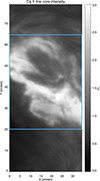 |
Fig. 1. Spatial distribution of the line core intensity signals for the Ca II spectral line. The blue box indicates the field-of-view selected for the analysis presented in this publication. |
3. Results
3.1. Spatial distribution of polarisation signals
We started the analysis of the spectral features of the region where the X-flare event takes place by examining the evolution of several reference quantities. In particular, we studied the spatial distribution of the line core intensity and maximum circular polarisation signals. We focused on the Ca II 854.2 nm spectral line only because, as shown in our previous work, there is almost no trace of flaring activity in the photospheric line. Focusing on one transition will also reduce the number of plots included in the manuscript, simplifying the visualisation of the most critical aspects related to the evolution of the flare. Furthermore, as mentioned in the previous work, linear polarisation signals are very weak for the Ca II transition, so we also chose not to plot them.
We display the results for the spatial evolution of the line core intensity in Figure 2. There, we can see that the first snapshots of the observation show an extended region where the line core intensity is in emission (see white areas), as found in our previous study. The area of enhanced intensity is gradually fading as we examine additional snapshots (the cadence is around 10 minutes) until we see a much weaker presence of enhanced line core intensity signals over a much smaller spatial area.
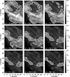 |
Fig. 2. Evolution of the spatial distribution of the line core intensity signals for the Ca II spectral line. The time difference between panels is around 10 min. Contours designate the areas where the line core intensity of the Ca II transition is equal to or higher than 1.1 of the Ic for each snapshot. |
As a reference, we present in Figure 3 the evolution of the pixel count in the ribbon area. We defined this ribbon area as the locations where the line core intensity of the Ca II transition is in emission with an intensity equal to or larger than 1.1 of Ic. The initial snapshot reveals a substantial number of pixels within the ribbon area, approximately 9 × 104 pixels. This pixel count decreases rapidly, dropping to around 2 × 104 pixels by the fifth snapshot, a reduction by a factor of 4.5. Following this sharp decline, the situation stabilises, as indicated by the flattening of the curve, which suggests that the most energetic processes occur in the first minutes after the start of the observation, which coincides with the flare peak flare.
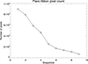 |
Fig. 3. Evolution of pixel count over time. The pixel count for each snapshot corresponds to the pixels within the contours presented in Figure 2. |
We continue with the spatial distribution of the maximum circular polarisation signals in Figure 4. The first snapshot shows an apparent concentration of circular polarisation signals co-spatial with the location of the largest intensity signals at line core wavelengths. Also, as before, the strength of the maximum polarisation signals and the spatial area they occupy becomes weaker and weaker as time progresses. In addition, there are no strong V signals in any other areas of the observed FOV at any time of the observation time series.
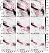 |
Fig. 4. Evolution of the spatial distribution of the maximum circular polarisation signals for the Ca II spectral line 854.1 nm. The time difference between panels is around 10 min. White areas represent regions with low polarisation signals, while darker regions designate areas with large circular polarisation signals. Contours designate the areas where the line core intensity of the Ca II transition is equal to or higher than 1.1 of the Ic for each snapshot (see also Fig. 2). |
3.2. Evolution of the atmospheric parameters
After inverting all the snapshots with DeSIRe using the same configuration as Ferrente et al. (2024), we analysed the evolution of the atmospheric parameters: temperature, line-of-sight (LOS) velocity, magnetic field strength, and inclination. Relying on our previous results (see the response function analysis in Ferrente et al. 2024), we focused on the evolution at log τ = −4 for regions outside the ribbon area, while we used atmospheric parameters at log τ = −3 within the ribbon contour. Our earlier studies revealed that the height of maximum sensitivity in flaring regions tends to shift toward deeper layers (i.e. log τ = −3). Although the ideal approach would be to compute the maximum of the RFs for each pixel within the ribbon at every snapshot, this process is highly computationally demanding, so we leave the exact computation for follow-up studies.
Starting with the temperature, Figure 5 depicts its evolution over time across nine snapshots. Similarly as in Figure 2, the contour highlights the location of the ribbon, defined as the areas where the line core intensity of the Ca II transition is in emission with an intensity equal to or larger than 1.1 of Ic. The evolution of the physical parameter is shown from the initial observing time (Δt = 0 min) to the final snapshot (Δt = 68 min). We fixed the temperature values for the colour bar of all the snapshots to have a better reference with respect to the initial snapshot when the flare occurs. During this period, we observe a significant temperature decrease along the flare ribbon starting from the second snapshot (Δt = 8.5 min). By the sixth frame (Δt = 42.5 min), it becomes challenging to identify the flaring region due to the continued temperature decline. Nevertheless, some pixels hotter than their surroundings can be found inside the areas highlighted by the contours.
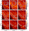 |
Fig. 5. Evolution of the spatial distribution of temperature at log τ = −4 for the pixels located outside the contour and at log τ = −3 for the pixels located inside the contour, over time. Contours designate the areas where the line core intensity of the Ca II transition is equal to or higher than 1.1 of the Ic for each snapshot (see also Fig. 2). The colored squares represent patches where we analyse the evolution of the physical parameters later on. |
In the case of the LOS velocity (Figure 6), we initially have strong upward velocities (blue regions) filling the area of the ribbon, as highlighted by the contour. These regions of strong upflows are enclosing areas where the amplitude of the LOS velocity is lower. In addition, the latter areas with weak velocities correspond to the regions where the temperature is highest, as observed by comparing with Figure 5, and to a double protrusion structure of opposite polarity within the FOV (see Ferrente et al. 2024, for more information). The evolution of the areas with high LOS velocity is interesting as the strong upward velocity regions expand towards the higher temperature areas, eventually filling them as their temperature is reduced with time. Moreover, these upflow regions shrink as time evolves, and by the end of our observation, only the high-intensity regions (corresponding to the location of the ribbon) show strong upflows. Notably, by the end of the time series, all the blue pixels, indicating upward velocities, are contained within the contour, marking the flare ribbon’s location from the intensity maps. Also, no sign of downward velocities can be found in any area or at any time.
Regarding magnetic field strength (see Figure 7), the first snapshot shows higher field strength values in the flare ribbon area, which correlates with the maximum circular polarisation signals seen in Figure 4 and with the maximum temperature values in Figure 5. As time progresses, the region with enhanced magnetic field strength decreases in area, splitting into two smaller subregions (e.g. Δt = 34 min) that follow the ribbon’s evolution (see contours), with values up to 1400 G persisting until the last snapshot.
Considering the inclination (Figure 8), the FOV is mainly characterised by nearly vertical (with respect to the solar surface) negative polarity (γ ∼ 150 degrees) areas. In contrast, the two protrusion regions at approximately [20, 50] arcsec exhibit the opposite polarity (γ ∼ 20 degrees). Compared with the rest of the examined atmospheric parameters, there are no significant changes with time in the inclination. Although it seems that within the contour representing the flaring region, the magnetic field remains vertical, whereas in areas where the ribbon disappears, it becomes more horizontal.
In order to have a more quantitative analysis of the evolution of the physical parameters, we studied the evolution of the flaring region by performing a statistical analysis. Initially, we considered all the values of the atmospheric parameters within the flare ribbon area, defined by the contours where the line core intensity of the calcium spectral line is equal to or higher than 1.1 of Ic. However, evaluating the mean values of these parameters within the ribbon yielded unsatisfactory results due to excessively high standard deviations. We suppose the reason is that there are significant small-scale variations in the atmosphere between different pixels inside what we defined as a flare ribbon. We also believe we could improve this selection criterion by focusing, for example, on a certain noise threshold for the polarisation signals instead. However, this method would also include pixels from many areas in the field of view that may not correspond to the same physical scenario, for example, the flare ribbon, the penumbra of the sunspot or the patches with opposite magnetic field polarities.
We analysed small-scale patches within the observed FOV corresponding to specific physical scenarios to address this limitation. The patches are highlighted with differently colored boxes in the figures that show the evolution of the atmospheric parameters. However, this process was also iterative because although we began with smaller patches of 10 × 10 pixels2, we still had that the average values showed high standard deviations. Thus, we reduced the patch size to 5 × 5 pixels2 without success, as the physics within each patch remained slightly heterogeneous. Ultimately, we settled on using 3 × 3 pixels2 patches (corresponding to 0.081 × 0.081 arcsec2), which produced more reasonable standard deviation values. Thus, we note here that the properties of the flare region change substantially in small-scale ranges, as small as a few arcsecs. However, these variations could be caused by the fact that we are averaging the atmospheric parameters for a single optical depth.
Regarding the specific physical scenarios, we selected five patches in various regions of interest. The blue patch corresponds to an area of low polarisation signals and weak magnetic activity. The red patch belongs to an area with moderate polarisation signals where the inferred magnetic fields are horizontal with respect to the solar surface. This patch is located in between two opposite magnetic field polarities. The purple patch is situated in a region with moderate polarisation signals, and the inferred magnetic field is almost vertical with respect to the solar surface but with a polarity opposite to that of the surrounding areas. The green patch belongs to the central part of the flare ribbon, where the intensity profiles at line core wavelengths are in emission and where the inferred temperatures are the hottest of the entire FOV. Finally, the orange patch is located in a region with moderate polarisation signals, and the inferred temperatures are low compared with the flare ribbon area. However, this patch shows strong upward velocities for the entire observation timespan despite displaying a low temperature.
Note that, with evolving time, some among the region belonging to the ribbon end outside the ribbon area (e.g. orange patch), so that for these patches we changed the optical depth at which physical parameters are evaluated from log τ = −3 to log τ = −4.
We show in Figure 9 the evolution of various atmospheric parameters for the five patches mentioned above. Starting with the temperature (upper-left panel), all patches, except the green one, maintain an almost constant temperature in the range between 6000–8000 K with low standard deviations. The green patch, located in the region with the highest temperature enhancement, exhibits a sharp decrease in temperature, reaching values closer to the rest of the patches from snapshot number 4. The green patch also shows higher standard deviations in the first three snapshots than in subsequent ones.
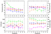 |
Fig. 9. Evolution of the atmospheric parameters belonging to the areas highlighted with colour in Figure 5. The top row, from left to right, shows the evolution of the temperature and LOS velocity, while the bottom row, from left to right, shows the evolution of the magnetic field strength and inclination. |
In the case of the LOS velocity (upper-right panel), the red, purple, and blue patches display small velocities near zero. In contrast, the orange and green patches exhibit the opposite behaviour: the orange patch starts with strong upward (with respect to the solar surface) velocities, approaching zero by the fifth snapshot, while the green patch transitions from near-zero velocity at the beginning to strong upward velocities from the fourth snapshot onwards.
Regarding magnetic field strength (bottom-left panel), all patches have high standard deviations, with values varying with time. In addition, the green patch corresponding to the highest temperature region shows larger field strength values than the rest of the selected patches.
In the case of the evolution of the magnetic field inclination (bottom-right panel), the blue and red patches show almost constant inclination throughout the entire time series, centred around γ ≈ 100 degrees. The orange and green patches start with a vertical inclination in the negative direction (γ ∼ 160−170 degrees). The orange patch becomes more horizontal by the fourth snapshot, reaching γ ∼ 90 degrees by the sixth snapshot. The pink patch, selected from the region with opposite polarity, starts with an inclination of γ ∼ 30 degrees and a significant standard deviation, increasing to γ = 50 degrees from the third snapshot, with lower standard deviation after that.
4. Discussion
The analysis carried out in this work evidences that during the flare evolution a rapid reduction in the area of enhanced intensity occurred. We suppose that this behaviour can be ascribed to the confined nature of the flare and the lack of ribbon separation (Ferrente et al. 2023). This absence of ribbon separation suggests that magnetic reconnection is not progressing to successively higher coronal loops, keeping the flare confined to a localized region without the expansion seen in eruptive events. Notably, Thalmann et al. (2015) studied the evolution of the free energy for this event, estimating the free magnetic energy at approximately 1.5 × 1026 J before the flare. They also found that a similar amount of free energy was restored afterward, indicating that the active region efficiently replenished its magnetic energy. This energy replenishment highlights the potential of this active region to produce subsequent flares of comparable magnitude, a behavior observed in AR12192, which produced several major flares in succession. The unchanged free energy further suggests that there was no large-scale reconfiguration of the magnetic field, a characteristic typically seen in eruptive events.
Additionally, the reduction in ribbon size, especially in the Ca II 854.2 nm line at 1.1 Ic could be linked to the flare transitioning into its gradual phase. As the flare evolves, chromospheric cooling lowers the temperature of the heated plasma, which may reduce the intensity and cause the ribbon area in Ca II 854.2 nm to shrink due to diminished chromospheric heating. Moreover, during the gradual phase of confined flares, energy release typically weakens (Svetska 1990). This decrease in energy input, through reduced non-thermal electron precipitation and thermal conduction from the corona, leads to lower chromospheric temperatures and densities, further diminishing the brightness and spatial extent of the flare ribbons in Ca II 854.2 nm.
In the previous publication of this series, we pointed out the apparent correlation between areas with enhanced temperature at log τ = −4 and the lack of LOS velocities at the same locations. A behaviour that we have found again on different snapshots (i.e. at different times). We rechecked the profiles, and although the Stokes I parameter is in emission and quite complex in general, we have that the Doppler shift of the line core is small for those pixels. The same happens with the zero-crossing of the Stokes V parameter, which is almost at the rest wavelength. Thus, we believe the inversion results provide consistent LOS velocities regarding spectral Doppler shifts. However, we are still unable to explain why the hottest areas would have to show the lowest LOS velocities. Therefore, we plan to continue exploring the properties of solar flares through NLTE inversions of the full Stokes vector of additional observations. In particular, we want to analyse data from a different type of instrument, like a long slit spectrograph, that could provide new insights into this unexpected behaviour. We understand that the dynamic nature of flares is not best suited for long-slit instruments, but, at the same time, the spectral coverage is better, which may help find additional clues. The Gregor Infrared Spectrograph (Collados et al. 2012) installed at the Gregor telescope (Schmidt et al. 2012; Kleint et al. 2020) have been recently upgraded to support multi-channel observations of complementary spectral lines (Quintero Noda et al. 2022), in particular, the same Ca II 854.2 nm transition used in this work. Also, the Sunrise Chromospheric Spectropolarimeter (Katsukawa et al. 2020) on board of the balloon-borne Sunrise telescope (Solanki et al. 2010) is designed to observe the same spectral line (Quintero Noda et al. 2016, 2017). We are aware that both instruments have observed different classes of flares in 2024. Hence, we hope to analyse their observations in the future when they are publicly available to compare the results with those presented here and in our previous work. In addition, we aim to look at theoretical models that could help us pinpoint this unexpected behaviour for the LOS velocity. We are aware of 3D magneto-hydrodynamic (MHD) simulations as those presented in Cheung et al. (2019) or Rempel et al. (2023) that successfully reproduce the flaring corona. As some of the snapshots are publicly available, we aim to analyse them in future work, focusing on the chromosphere to determine whether we can explain our findings.
Regarding the standard deviation of the atmospheric parameters, we found that when computing the average of a given atmospheric parameter at a given optical depth, the standard deviation of the result was high as soon as we considered areas of a few arcsec. This could indicate that the flaring region has a well-defined, small-scale, patchy structure that is in high contrast with its surroundings, which is very interesting indeed. Interestingly, some works based on observations of the Si IV transition with the IRIS mission (De Pontieu et al. 2014) seem to reveal a similar clustering tendency of just a few arcsec too (e.g. Ashfield et al. 2022, and references within). Moreover, we are also computing the average of different spatial locations at the same optical depth, which can lead to large deviations in the atmospheric parameters if the average height of formation of the fitted transitions changes abruptly in short spatial scales, a behaviour that we can find in Figure 8 of Ferrente et al. (2024).
Finally, in Figure 9 we see that the temperature in pixels belonging to the flare ribbon drops from an initial average of 10 kK to about 7 kK in just a few minutes. Post-flare cooling in the corona typically involves both conductive and radiative cooling (Culhane et al. 1970; Cargill et al. 1995; Aschwanden & Alexander 2001; Fletcher et al. 2011). Early on, conductive cooling dominates as heat is efficiently transported from the hot flare loops to the cooler, denser chromosphere along magnetic field lines, while radiative cooling becomes more significant at later stages when the temperature drops and the plasma density increases, thereby enhancing radiative losses. In our study, however, the observed temperature decrease in the chromosphere appears to be dominated by radiative cooling, which is consistent with its high-density environment. At these densities (ne ∼ 1012–1015 cm−3; Gingerich et al. 1971; Fontenla et al. 1993, 2006), the radiative cooling timescale scales as τrad ∝ ne−2, making radiative losses extremely efficient through strong emission lines such as Hα, Ca II, and Mg II. Meanwhile, conductive cooling is negligible in the chromosphere because thermal conduction is orders of magnitude less efficient than radiative losses in such dense plasma. Moreover, even though the inversions were computed under the assumption of thermodynamic equilibrium, they yield electron densities of around 1013 cm−3, which further supports the dominance of radiative cooling in the observed context.
5. Summary
We expanded our previous work analysing the evolution of reference spectral features, and by performing NLTE inversions of the full Stokes vector of an observation of an X-class solar flare for multiple snapshots covering around one hour of solar time. Thanks to the low computational inversion time of DeSIRe, we could use the same state-of-the-art methodology as our first work to obtain accurate fits of the full Stokes vector over a large FOV of 50 × 35 arcsec2.
Regarding the Stokes profiles, we find that the regions with enhanced line core intensity of the Ca II 854.2 nm transition slowly fade away as time passes, indicating that the flaring activity gets reduced from the start of the observations. The process is continuous, with each consecutive snapshot showing smaller areas with enhanced intensity signals. The same behaviour can be found for the areas with strong Stokes V signals, that is, they are more common and have high amplitude signals at the beginning of the observation and fade as time passes.
Regarding the evolution of the atmospheric parameters, our analysis indicates that some localised areas show temperature values that are much higher than their surroundings. These areas correspond to the pixels with the highest line core intensity signals. As time passes, those high-temperature regions occupy fewer and fewer areas until they almost vanish one hour after the start of the observation (that roughly coincides with the peak of the flare activity). Regarding the LOS velocity, we have material moving towards the solar surface in enhanced line core intensity areas. Only the hottest areas show a different LOS velocity, that is, a low amplitude velocity, similar to what we found in our previous work when analysing the first snapshot only. The magnetic field strength seems correlated with higher temperature regions with values around 1–1.5 kG. Concerning the magnetic field inclination, we have a much more subtle evolution, with fewer changes in the spatial distribution that is dominated by vertical fields of almost 180 degrees that enclose a complex feature that is nearly vertical but with opposite polarity.
We also examine in detail the evolution of the atmospheric parameters for specific areas over the FOV, like a region with low magnetic activity, an area with horizontal magnetic fields along the polarity inversion line, a structure characterised by magnetic fields with positive polarity, a patch situated in an area with enhanced temperature and within the flare ribbon, and an area from a region with strong upward velocities. The values of most atmospheric parameters in the areas of interest generally remained almost constant. However, in the case of the area belonging to the flare ribbon, the temperature abruptly dropped after about 20 minutes, and we also detected an increase in the LOS velocity as the temperature decreased.
We highlighted in our previous work the importance of studying the evolution of the process to understand better the physics of an X-class flare. In that sense, the takeaway of this one-hour-long observation is that, generally, the behaviour of the atmospheric parameters in the lower atmosphere during the gradual phase is smooth, with a continuous reduction of the area they occupy and the amplitude of the phenomena. No re-appearance of hot regions or strong LOS velocities was found, indicating that after the abrupt impact of the X-class flare, the solar atmosphere slowly returned to a relaxed state in less than one hour. The confined nature of this flaring event probably played a significant role in its minimal impact in the post-flare phase. The flare did not cause a large-scale rearrangement of the magnetic fields or any material ejection. This confinement limited the energy release and subsequent atmospheric disruptions, leading to a smoother and quicker relaxing phase.
We learned more about flares, an interesting solar phenomenon. We hope to continue working on this topic to expand our knowledge of solar flares further. In particular, we want to explore spectropolarimetric observations of different types of instruments and combine those results with observations of different atmospheric layers, such as the transition region and the corona. In addition, we need to complement these observational works with theoretical studies, in particular, recent 3D MHD simulations of solar flares.
Acknowledgments
We thank an anonymous referee for his/her comments which helped us to improve the quality of this work. The research leading to these results has received funding from the European Union’s Horizon 2020 research and innovation program under grant agreement No.739500 (PRE-EST project) and No. 824135 (SOLARNET project). F. Ferrente and S.L. Guglielmino acknowledge support from ASI/INAF agreement n. 2022-29-HH.0 Missione MUSE. F. Ferrente and F. Zuccarello acknowledge support by the Università degli Studi di Catania (PIA.CE.RI. 2020–2022 Linea 2) and by the Italian MIUR-PRIN grant 2017APKP7T on “Circumterrestrial Environment: Impact of Sun-Earth Interaction”. This research was carried out in the framework of the CAESAR (Comprehensive spAce wEather Studies for the ASPIS prototype Realization) project, supported by the Italian Space Agency and the National Institute of Astrophysics through the ASI-INAF agreement no. 2020-35-HH.0 for the development of the ASPIS (ASI Space weather InfraStructure) prototype of scientific data center for Space Weather. C. Quintero Noda acknowledges support from the Agencia Estatal de Investigación del Ministerio de Ciencia, Innovación y Universidades (MCIU/AEI) under grant “Polarimetric Inference of Magnetic Fields” and the European Regional Development Fund (ERDF) with reference PID2022-136563NB-I00/10.13039/501100011033. The publication is part of the Project ICTS2022-007828, funded by MICIN and the European Union NextGenerationEU and the RTRP. We also thank Dr. Serena Criscuoli for providing the IBIS calibrated data. SLG acknowledges support from Italian Space Agency and the Ministry of University and Research under Contract n. 2024-5-E.0 (Space It Up) and support from INAF through Bando per il finanziamento della Ricerca Fondamentale 2023–IDEA-SW project. The National Solar Observatory is operated by the Association of Universities for Research in Astronomy, Inc.(AURA) under cooperative agreement with the National Science Foundation. The SDO/HMI data used in this paper are courtesy of NASA/SDO and the HMI science team. Use of NASA’s Astrophysical Data System is gratefully acknowledged. Facilities: DST (IBIS), SDO (HMI).
References
- Antonucci, E., Gabriel, A. H., & Dennis, B. R. 1984, ApJ, 287, 917 [NASA ADS] [CrossRef] [Google Scholar]
- Aschwanden, M. J., & Alexander, D. 2001, Sol. Phys., 204, 91 [NASA ADS] [CrossRef] [Google Scholar]
- Ashfield, I., W. H., Longcope, D. W., Zhu, C., & Qiu, J. 2022, ApJ, 926, 164 [Google Scholar]
- Asplund, M., Grevesse, N., Sauval, A. J., & Scott, P. 2009, ARA&A, 47, 481 [NASA ADS] [CrossRef] [Google Scholar]
- Bornmann, P. L. 1999, in The many faces of the sun: a summary of the results from NASA’s Solar Maximum Mission, eds. K. T. Strong, J. L. R. Saba, B. M. Haisch, & J. T. Schmelz, 301 [Google Scholar]
- Cameron, R., & Sammis, I. 1999, ApJ, 525, L61 [Google Scholar]
- Cargill, P. J., Mariska, J. T., & Antiochos, S. K. 1995, ApJ, 439, 1034 [NASA ADS] [CrossRef] [Google Scholar]
- Carmichael, H. 1964, NASA Spec. Publ., 50, 451 [NASA ADS] [Google Scholar]
- Castellanos Durán, J. S., Kleint, L., & Calvo-Mozo, B. 2018, ApJ, 852, 25 [Google Scholar]
- Cavallini, F. 2006, Sol. Phys., 236, 415 [NASA ADS] [CrossRef] [Google Scholar]
- Cheng, J. X., Kerr, G., & Qiu, J. 2012, ApJ, 744, 48 [Google Scholar]
- Cheung, M. C. M., Rempel, M., Chintzoglou, G., et al. 2019, Nat. Astron., 3, 160 [NASA ADS] [CrossRef] [Google Scholar]
- Collados, M., Lagg, A., Díaz García, J. J., et al. 2007, in The Physics of Chromospheric Plasmas, eds. P. Heinzel, I. Dorotovič, & R. J. Rutten, ASP Conf. Ser., 368, 611 [Google Scholar]
- Collados, M., López, R., Páez, E., et al. 2012, Astron. Nachr., 333, 872 [Google Scholar]
- Culhane, J. L., Vesecky, J. F., & Phillips, K. J. H. 1970, Sol. Phys., 15, 394 [NASA ADS] [CrossRef] [Google Scholar]
- de la Cruz Rodríguez, J., Leenaarts, J., Danilovic, S., & Uitenbroek, H. 2019, A&A, 623, A74 [Google Scholar]
- De Pontieu, B., Title, A. M., Lemen, J. R., et al. 2014, Sol. Phys., 289, 2733 [Google Scholar]
- Dunn, R. B. 1969, S&T, 38, 368 [NASA ADS] [Google Scholar]
- Ermolli, I., Giorgi, F., Murabito, M., et al. 2022, A&A, 661, A74 [NASA ADS] [CrossRef] [EDP Sciences] [Google Scholar]
- Ferrente, F., Zuccarello, F., Guglielmino, S. L., Criscuoli, S., & Romano, P. 2023, ApJ, 954, 185 [NASA ADS] [CrossRef] [Google Scholar]
- Ferrente, F., Quintero Noda, C., Zuccarello, F., & Guglielmino, S. L. 2024, A&A, 686, A244 [NASA ADS] [CrossRef] [EDP Sciences] [Google Scholar]
- Fletcher, L., Dennis, B. R., Hudson, H. S., et al. 2011, Space Sci. Rev., 159, 19 [Google Scholar]
- Fontenla, J. M., Avrett, E. H., & Loeser, R. 1993, ApJ, 406, 319 [Google Scholar]
- Fontenla, J. M., Avrett, E., Thuillier, G., & Harder, J. 2006, ApJ, 639, 441 [Google Scholar]
- Gafeira, R., Orozco Suárez, D., Milić, I., et al. 2021, A&A, 651, A31 [NASA ADS] [CrossRef] [EDP Sciences] [Google Scholar]
- Gingerich, O., Noyes, R. W., Kalkofen, W., & Cuny, Y. 1971, Sol. Phys., 18, 347 [Google Scholar]
- Handy, B. N., Acton, L. W., Kankelborg, C. C., et al. 1999, Sol. Phys., 187, 229 [Google Scholar]
- Harvey, J. W., Hill, F., Hubbard, R. P., et al. 1996, Science, 272, 1284 [Google Scholar]
- Hirayama, T. 1974, Sol. Phys., 34, 323 [Google Scholar]
- Katsukawa, Y., del Toro Iniesta, J. C., Solanki, S. K., et al. 2020, in Ground-based and Airborne Instrumentation for Astronomy VIII, eds. C. J. Evans, J. J. Bryant, & K. Motohara, SPIE Conf. Ser., 11447, 114470Y [Google Scholar]
- Kleint, L. 2017, ApJ, 834, 26 [Google Scholar]
- Kleint, L., Berkefeld, T., Esteves, M., et al. 2020, A&A, 641, A27 [EDP Sciences] [Google Scholar]
- Kopp, R. A., & Pneuman, G. W. 1976, Sol. Phys., 50, 85 [Google Scholar]
- Kosovichev, A. G., & Zharkova, V. V. 1999, Sol. Phys., 190, 459 [Google Scholar]
- Kosovichev, A. G., & Zharkova, V. V. 2001, ApJ, 550, L105 [CrossRef] [Google Scholar]
- Kuckein, C., Collados, M., Sainz, R. M., & Ramos, A. A. 2015, in Polarimetry, ed. K. N. Nagendra, S. Bagnulo, R. Centeno, & M. Jesús Martínez González, 305, 73 [NASA ADS] [Google Scholar]
- Kuridze, D., Henriques, V., Mathioudakis, M., et al. 2017, ApJ, 846, 9 [Google Scholar]
- Lemen, J. R., Title, A. M., Akin, D. J., et al. 2012, Sol. Phys., 275, 17 [Google Scholar]
- Neupert, W. M. 1968, ApJ, 153, L59 [NASA ADS] [CrossRef] [Google Scholar]
- Petrie, G. J. D. 2019, ApJS, 240, 11 [NASA ADS] [CrossRef] [Google Scholar]
- Qiu, J., & Cheng, J. 2022, Sol. Phys., 297, 80 [Google Scholar]
- Quintero Noda, C., Shimizu, T., de la Cruz Rodríguez, J., et al. 2016, MNRAS, 459, 3363 [Google Scholar]
- Quintero Noda, C., Shimizu, T., Katsukawa, Y., et al. 2017, MNRAS, 464, 4534 [NASA ADS] [CrossRef] [Google Scholar]
- Quintero Noda, C., Collados, M., Regalado Olivares, S., et al. 2022, in Ground-based and Airborne Instrumentation for Astronomy IX, eds. C. J. Evans, J. J. Bryant, & K. Motohara, SPIE Conf. Ser., 12184, 121840U [Google Scholar]
- Rempel, M., Chintzoglou, G., Cheung, M. C. M., Fan, Y., & Kleint, L. 2023, ApJ, 955, 105 [NASA ADS] [CrossRef] [Google Scholar]
- Ruiz Cobo, B., Quintero Noda, C., Gafeira, R., et al. 2022, A&A, 660, A37 [NASA ADS] [CrossRef] [EDP Sciences] [Google Scholar]
- Saba, J. L. R., Gaeng, T., & Tarbell, T. D. 2006, ApJ, 641, 1197 [Google Scholar]
- Scherrer, P. H., Bogart, R. S., Bush, R. I., et al. 1995, Sol. Phys., 162, 129 [Google Scholar]
- Scherrer, P. H., Schou, J., Bush, R. I., et al. 2012, Sol. Phys., 275, 207 [Google Scholar]
- Schmidt, W., von der Lühe, O., Volkmer, R., et al. 2012, Astron. Nachr., 333, 796 [Google Scholar]
- Schou, J., Scherrer, P. H., Bush, R. I., et al. 2012, Sol. Phys., 275, 229 [Google Scholar]
- Shine, R. A., & Linsky, J. L. 1974, Sol. Phys., 39, 49 [NASA ADS] [CrossRef] [Google Scholar]
- Simões, P. J. A., Reid, H. A. S., Milligan, R. O., & Fletcher, L. 2019, ApJ, 870, 114 [Google Scholar]
- Solanki, S. K., Barthol, P., Danilovic, S., et al. 2010, ApJ, 723, L127 [NASA ADS] [CrossRef] [Google Scholar]
- Stenflo, J. O. 2013, A&ARv, 21, 66 [NASA ADS] [CrossRef] [Google Scholar]
- Sturrock, P. A., & Coppi, B. 1966, ApJ, 143, 3 [NASA ADS] [CrossRef] [Google Scholar]
- Sudol, J. J., & Harvey, J. W. 2005, ApJ, 635, 647 [Google Scholar]
- Svetska, Z. 1990, in New Windows to the Universe, ed. F. Sanchez, & M. Vazquez, 99 [Google Scholar]
- Thalmann, J. K., Su, Y., Temmer, M., & Veronig, A. M. 2015, ApJ, 801, L23 [NASA ADS] [CrossRef] [Google Scholar]
- Uitenbroek, H. 2006, in Solar MHD Theory and Observations: A High Spatial Resolution Perspective, eds. J. Leibacher, R. F. Stein, & H. Uitenbroek, ASP Conf. Ser., 354, 313 [NASA ADS] [Google Scholar]
- Wang, H. 1992, Sol. Phys., 140, 85 [NASA ADS] [CrossRef] [Google Scholar]
- Wang, H., Ewell, M. W., Jr, Zirin, H., & Ai, G. 1994, ApJ, 424, 436 [Google Scholar]
- Warren, H. P. 2001, in AGU Spring Meeting Abstracts, Spring Meeting 2001, SP42A-12 [Google Scholar]
- Yadav, R., Díaz Baso, C. J., de la Cruz Rodríguez, J., Calvo, F., & Morosin, R. 2021, A&A, 649, A106 [NASA ADS] [CrossRef] [EDP Sciences] [Google Scholar]
All Tables
All Figures
|
Fig. 1. Spatial distribution of the line core intensity signals for the Ca II spectral line. The blue box indicates the field-of-view selected for the analysis presented in this publication. |
| In the text | |
|
Fig. 2. Evolution of the spatial distribution of the line core intensity signals for the Ca II spectral line. The time difference between panels is around 10 min. Contours designate the areas where the line core intensity of the Ca II transition is equal to or higher than 1.1 of the Ic for each snapshot. |
| In the text | |
|
Fig. 3. Evolution of pixel count over time. The pixel count for each snapshot corresponds to the pixels within the contours presented in Figure 2. |
| In the text | |
|
Fig. 4. Evolution of the spatial distribution of the maximum circular polarisation signals for the Ca II spectral line 854.1 nm. The time difference between panels is around 10 min. White areas represent regions with low polarisation signals, while darker regions designate areas with large circular polarisation signals. Contours designate the areas where the line core intensity of the Ca II transition is equal to or higher than 1.1 of the Ic for each snapshot (see also Fig. 2). |
| In the text | |
|
Fig. 5. Evolution of the spatial distribution of temperature at log τ = −4 for the pixels located outside the contour and at log τ = −3 for the pixels located inside the contour, over time. Contours designate the areas where the line core intensity of the Ca II transition is equal to or higher than 1.1 of the Ic for each snapshot (see also Fig. 2). The colored squares represent patches where we analyse the evolution of the physical parameters later on. |
| In the text | |
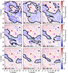 |
Fig. 6. Same as Figure 5 but for the LOS velocity. |
| In the text | |
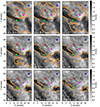 |
Fig. 7. Same as Figure 5 but for the magnetic field strength. |
| In the text | |
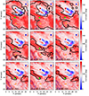 |
Fig. 8. Same as Figure 5 but for the magnetic field inclination. |
| In the text | |
|
Fig. 9. Evolution of the atmospheric parameters belonging to the areas highlighted with colour in Figure 5. The top row, from left to right, shows the evolution of the temperature and LOS velocity, while the bottom row, from left to right, shows the evolution of the magnetic field strength and inclination. |
| In the text | |
Current usage metrics show cumulative count of Article Views (full-text article views including HTML views, PDF and ePub downloads, according to the available data) and Abstracts Views on Vision4Press platform.
Data correspond to usage on the plateform after 2015. The current usage metrics is available 48-96 hours after online publication and is updated daily on week days.
Initial download of the metrics may take a while.