| Issue |
A&A
Volume 696, April 2025
|
|
|---|---|---|
| Article Number | L3 | |
| Number of page(s) | 13 | |
| Section | Letters to the Editor | |
| DOI | https://doi.org/10.1051/0004-6361/202554027 | |
| Published online | 02 April 2025 | |
Letter to the Editor
Extremely iron-poor O-type stars in the Magellanic Bridge
1
Zentrum für Astronomie der Universität Heidelberg, Astronomisches Rechen-Institut, Mönchhofstr. 12–14, 69120 Heidelberg, Germany
2
Department of Astronomy, University of Wisconsin, 475 N. Charter St., Madison, WI 53706, USA
3
Department of Physics and Astronomy, Macalester College, 1600 Grand Ave, St. Paul, MN 55105, USA
4
Institut für Physik und Astronomie, Universität Potsdam, Karl-Liebknecht-Str. 24/25, 14476 Potsdam, Germany
⋆ Corresponding author; This email address is being protected from spambots. You need JavaScript enabled to view it.
Received:
4
February
2025
Accepted:
13
March
2025
Abstract
Context. To study stars analogous to those in the early Universe with redshift z > 3, we need to probe environments with low metallicities. Until recently, massive O-type stars with a metallicity lower than that of the Small Magellanic Cloud (SMC; Z < 20% Z⊙) were only known in compact dwarf galaxies. The signal-to-noise ratio and spatial resolution of observations of stars in such distant galaxies (> 1 Mpc) are limited. Recently, a few O-type stars were identified in the nearby Magellanic Bridge. This is a unique laboratory with a low gas density and low metal content.
Aims. We acquired high-resolution HST-COS far-UV spectra of two O-type stars in the Magellanic Bridge. Using the UV forest of iron lines from these observations, we measured the inherent iron abundances precisely and determined the metallicity of the stars.
Methods. Using detailed expanding nonlocal thermal equilibrium atmosphere models, we generated synthetic spectra for different iron abundances and for a range of microturbulent velocities. We used Bayesian posterior sampling to measure the iron abundance and compute the uncertainties based on the possible range of microturbulent velocities.
Results. The O stars in the Magellanic Bridge have severely sub-SMC iron abundances that reach as low as 10.8% and 3.6% Fe⊙. The most Fe-deficient star also shows α-enhancement. These stars are the nearest extremely metal-poor O stars discovered to date.
Conclusions. Our finding marks the first robust determination of O-star iron abundances in a metallicity regime comparable to dwarf galaxies such as Sextans A and Leo P. The iron abundances of the stars do not correlate with their oxygen abundances. Our results highlight the problem of using oxygen-based metallicities. The proximity of the stars in the Bridge combined with their different abundance patterns underlines that the interstellar medium of the Magellanic Bridge must be highly inhomogeneous and is not properly mixed.
Key words: stars: abundances / stars: atmospheres / stars: early-type / stars: fundamental parameters / stars: massive / Magellanic Clouds
© The Authors 2025
 Open Access article, published by EDP Sciences, under the terms of the Creative Commons Attribution License (https://creativecommons.org/licenses/by/4.0), which permits unrestricted use, distribution, and reproduction in any medium, provided the original work is properly cited.
This article is published in open access under the Subscribe to Open model. This email address is being protected from spambots. You need JavaScript enabled to view it. to support open access publication.
1. Introduction
Massive stars (Minit > 8 M⊙) play an important role for the chemical enrichment and ionization of the Universe. Following the Big Bang, the first Population III stars formed from pristine gas clouds that almost entirely consisted of hydrogen and helium (e.g. Bromm et al. 2002). Through nuclear fusion, these hot massive stars produced heavier elements, primarily the α-peak elements, which were dispersed into the interstellar medium (ISM) via intrinsic mass loss and their final core-collapse supernovae (see e.g. Woosley et al. 2002; Janka et al. 2007, for a review). This seeded future generations of star formation.
The study of metal-poor massive stars that were born in environments with minimum prior chemical enrichment provides a unique window into the early stages of stellar evolution and nucleosynthesis. These stars are local analogs of the metal-poor stellar populations that are observed in high-redshift galaxies by the James Webb Space Telescope (JWST). The increasingly rich JWST spectroscopic observations of metal-deficient galaxies at high redshifts highlight the lack of a deeper quantitative understanding and problems in current models at low metallicity (see, e.g., Garg et al. 2024), for instance, when observed emission line ratios from ionized gas are interpreted (Matthee et al. 2023; Laseter et al. 2024; Rowland et al. 2025). As discussed by Hopkins et al. (2023), the interpretation of spatially integrated JWST spectra of most sources are expected to be affected by a variety of issues, such as dust absorption and ISM structure, as well as the properties of the stars. Massive star models grounded by observational data are essential for the analysis of optical spectra of young low-metallicity galaxies at high redshifts.
Empirical constraints from individual observed metal-poor massive stars predominantly stem from spectroscopic studies of stars in the Small Magellanic Cloud (SMC) with a mean metallicity of Z ∼ 20% Z⊙ (e.g. Bouret et al. 2003; Ramachandran et al. 2019; Rickard et al. 2022) or within the recent X-Shooting ULLYSES (XShootU) collaboration (Vink et al. 2023; Backs et al. 2024; Bernini-Peron et al. 2024). However, JWST observations of galaxies at redshift z > 3 reveal even lower metallicities up to ∼2% Z⊙ (e.g., Curti et al. 2024; Boyett et al. 2024). Therefore, it is essential to spectroscopically analyze stars in environments with sub-SMC metallicities to bridge the gap between theoretical predictions and high-z observations. While old, low-mass, and extremely metal-poor (Z < 10% Z⊙) stars can be found in the Milky Way and Galactic halo (e.g. Gratton & Sneden 1988; Cohen et al. 2008), young massive stars are missing there. A few massive stars with comparably low metallicities have been studied in comparatively distant (≳1 Mpc) compact dwarf galaxies such as Sextans A and Leo P (e.g., Evans et al. 2019; Garcia et al. 2019; Telford et al. 2024). The observations of individual massive stars in these distant locations have a limited signal-to-noise ratio and spatial resolution.
The Magellanic Bridge, which was first discovered by Hindman et al. (1963), is a stream of gas and mostly young stars that connects the two Magellanic Clouds. With its nearby distance of ∼55 kpc (Jacyszyn-Dobrzeniecka et al. 2016), low foreground extinction, low density, and low mean metal content (Lehner et al. 2001), the Magellanic Bridge is a unique alternative laboratory in our cosmic neighborhood in which we can study star formation and feedback at extremely low metallicity. Notably, Dufton et al. (2008) reported B stars in the Bridge with very low iron abundances.
The Magellanic Bridge contains a population of young stars (primarily B and A types; Rolleston et al. 1999), but the first three O-type stars were discovered only recently (Ramachandran et al. 2021). Two of them were found to have extremely low mean CNO abundances of 4% and 8% solar. However, a main element affecting the mass loss and therefore evolution of massive stars is iron (e.g., Abbott 1982; Chiosi & Maeder 1986). The iron abundance and opacity set the necessary conditions for launching the wind of massive stars and thus are the main ingredient of the scaling of the mass-loss rate with metallicity (e.g., Pauldrach 1987; Vink et al. 2001). However, in contrast to most metals that are promptly expelled to the ISM during the core collapse of massive stars, iron is mainly produced with a considerable time delay during type Ia supernovae. Thus, the iron abundance does not necessarily scale with other metal abundances. Differences between α/Fe have also been discovered for some massive stars, for example, in IC 1613 (Garcia et al. 2014). For hot OB stars, the determination of the iron abundance requires high-resolution UV spectra and is often unfeasible for distances larger than the distance to the Magellanic Clouds. Rapid rotation is common at low metallicity and further complicates an analysis by smearing the iron lines. The determined iron abundances are therefore often limited to cool supergiants with iron lines in the optical spectra (Urbaneja et al. 2023).
We use newly acquired HST UV spectra to measure the inherent iron abundances for the two O-type stars MBO2 and MBO3 in the Magellanic Bridge for the first time (Ramachandran et al. 2021). The two stars show low mean CNO abundances and slow rotation. To do this, we employ atmosphere models with low iron abundances and a newly developed Bayesian analysis framework.
2. Observations
The UV spectra (ID 16647; PI Ramachandran) of the two CNO metal poor O-type stars were taken with the grating G160M/1623 by the Cosmic Origins Spectrograph (COS; Green et al. 2012) on board the Hubble Space Telescope (HST). To assess the consistency of our approach, we reexamined the Fe abundance of one of the sample stars from Dufton et al. (2008, DI 1388), which is reported to have the lowest Fe content of only XFe = 1.26% XFe, ⊙. Instead of the HST-GHRS (grating G200M) spectra (1888−1929 Å) used by Dufton et al. (2008), our analysis is based on STIS/E140M spectra (ID 7511; PI Keenan), which have a higher resolution and signal-to-noise ratio.
A summary of the stellar coordinates, spectral types (from Ramachandran et al. 2021), and observational settings can be found in Table A.1. In Fig. 1 we highlight the location of the analyzed stars within the Magellanic Bridge with respect to the SMC and LMC. The basic data reduction (e.g., normalization and radial velocity correction) is described in Appendix A.
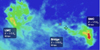 |
Fig. 1. Neutral hydrogen map of the Magellanic Clouds and the Magellanic Bridge from the HI4PI survey (HI4PI Collaboration 2016). The black plus marks the approximate position of MBO2 and MBO3 within the Magellanic Bridge, and the gray cross shows DI1388. |
3. Data analysis
3.1. Stellar atmosphere models
For the spectral analysis, we used the PoWR non-LTE expanding stellar atmosphere code (see, e.g., Gräfener et al. 2002; Hamann & Gräfener 2003; Sander et al. 2015), which calculates model atmospheres and generates synthetic spectra for a chosen set of wind and stellar parameters. PoWR accounts for line blanketing by grouping thousands of atomic energy levels from iron-group elements into superlevels (Gräfener et al. 2002). Adopting the parameters (e.g., Teff, log g, v sin i, and vmac) and abundances from Ramachandran et al. (2021) constrained from the optical regime, we calculated models with different iron abundances between 1 and 15% and varying microturbulent velocities (see Table D.1 for details of the atomic data). Instead of using the iron mass fraction directly, PoWR uses the iron-group abundance (herein denoted as G) as input parameter. This consists of scandium, titanium, vanadium, chromium, manganese, iron, cobalt, and nickel. The specific elemental abundances are calculated internally, weighted by their relative solar abundances. We did not analyze the wind features, but instead employed fixed values for the terminal wind velocities of v∞ = 1994 km s−1, and mass-loss rates of Ṁ = 10−9.0 M⊙ yr−1 and Ṁ = 10−8.5 M⊙ yr−1 for MBO2 and MBO3, respectively. Throughout this work, our reference for the solar abundances are the values from Asplund et al. (2009) and Scott et al. (2015a,b).
3.2. Determination of the microturbulence
The two stars MBO2 and MBO3 have very narrow lines. For MBO2, Ramachandran et al. (2021) were only able to determine upper limits for the microturbulence ξ, projected rotation velocity v sin i, and the macroturbulence vmac because the absorption lines are extremely narrow. As there is a known degeneracy between the Fe abundance and ξ (e.g., Bouret et al. 2015) when using the UV iron forest to determine Fe abundances, we examined a range of microturbulent velocities between 1 and 20 km s−1 that still reproduced the shape of the observed metal lines.
To determine the range of microturbulences that agreed with the observed spectrum, we compared the observed S Vλ1501.8 line with models calculated with a varying ξ (see Fig. 2). We used the S V line because it is the strongest and most isolated metal line in the considered UV spectral range. Microturbulence influences the broadened wings of these metal lines. While for MBO2, all models with ξ ≤ 5 km s−1 matched the wings of the absorption lines, viable microturbulence values for MBO3 are in the range of ξ = 5 − 10 km s−1. Ramachandran et al. (2021) determined a microturbulence of ξ ≤ 2 km s−1 for MBO2 and ξ = 8 km s−1 for MBO3. This agrees with these results. To later combine the fitting results for different ξ, we also quantified the fit to the S V line by computing the χ2 value (see Appendix B).
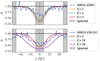 |
Fig. 2. Comparison of the observed and modeled S Vλ1501.76 line for different ξ for MBO2 (top) and MBO3 (bottom) in velocity space. The defined wing region in which we evaluated χ2 is highlighted. |
3.3. Bayesian inference of the iron abundances
It is difficult to visually distinguish the Fe lines from the noise level. A more advanced approach than fitting by eye is therefore required for an accurate determination of the Fe abundance. As described in Appendix A, a normalization of the UV spectra with synthetic models can require a small flux shift to the model continuum. This corresponds to a slight change in the stellar luminosity. Using Bayesian posterior sampling, we inferred the flux shift and Fe group abundance G by fitting the forest of Fe IV–V lines for a range of fixed ξ values. To sample the posterior distribution, we employed the Markov chain Monte Carlo (MCMC) algorithm emcee (Foreman-Mackey et al. 2013), assuming a Gaussian likelihood,
 (1)
(1)
and we used the estimated flux errors σi from the COS data products (Johnson et al. 2021).
The normalization varies across wavelengths likely due to instrumental effects, and a fit of the entire spectrum would require multiple shifts. We therefore restricted our fits to regions with a reliable normalization. Additionally, we ignored the parts of the spectrum in which the noise dominates and spectral regions with wind lines or other strong absorption lines. These ignored wavelength intervals are different for the two stars (see Appendix E) but were kept constant for all fits with different ξ.
We calculated a grid of PoWR models for each star with different iron metallicities. Eight models were spaced between 1% and 15% G⊙ for MBO2, and five models were spaced between 1% and 9% G⊙ for MBO3. We otherwise fixed the stellar parameters to the values determined from the optical spectrum by Ramachandran et al. (2021). To evaluate the spectrum at all metallicities within the grid, we used a linear interpolation between the points. We used uninformative prior distributions: For the iron abundance, we used a uniform prior in the interval given by the grid, and for the flux shift, we used a truncated Gaussian prior centered around μshift = 0 and with a standard deviation σshift = 10−14 in the interval [−3 × 10⁻¹⁴, 3 × 10⁻¹⁴] erg cm−2 s−1 Å−1. For each star, we ran ten chains with 10 000 steps. To confirm that the fits converged, we verified that the chain length was sufficiently (> 50 times) longer than the autocorrelation length τ. We discarded the first 1000 burn-in steps and thinned the samples so that we only considered each τ/2 step.
Finally, we computed the Fe abundance from the fraction of Fe in the G element (93%) and the total metallicity Z using the determined abundances for C, N, O, Mg, and Si from Ramachandran et al. (2021), plus our determined Fe abundance. The only missing element with a sufficient impact on Z is neon. No Ne line was detectable in the observed spectral range of the bridge stars. We therefore estimated the Ne number fraction from the O number fraction using a scaling factor of 1/5.2, as was determined for the H II region NGC 346 within the SMC (Valerdi et al. 2019).
4. Results and discussion
4.1. Metal-poor O stars MBO2 and MBO3
In Fig. 3 we compare the best-fit models with the observed Fe forest for MBO2 and MBO3. The microturbulence ξ was fixed to the values that best reproduce the observed S V line (see Fig. 2), that is, 2 km s−1 and 8 km s−1, respectively. In addition, we show a posterior predictive (PP) sample that is a set of simulated data points generated from the posterior distribution of the model parameters. This sample allowed us to assess the ability of the model to reproduce the observed data. The simulated and observed data agree well for both stars, indicating that the model successfully reproduces the key features of the observations within the uncertainties. The corresponding full spectra and corner plots for MBO2 and MBO3 can be found in Appendix E.
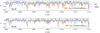 |
Fig. 3. Comparison of the observed (dashed blue line) and best-fit modeled (orange) Fe IV forest of lines for fixed microturbulence values of ξ = 2 km s−1 for MBO2 (top) and ξ = 10 km s−1 for MBO3 (bottom). The thickness of the orange model line represents the 3σ credible interval of the best-fit model. A PP sample is shown in light blue. The full spectral fits are given in Appendix E. |
To study the degeneracy between the ξ and Fe abundance, we also performed the fit for other ξ values. The detailed individual fitting results including the corner plots, and the corresponding spectra can be found in Appendix E. A summary of the fitting results is depicted in Fig. 4. As expected, the value for the iron abundance decreased when we assumed a stronger microturbulence. The derived iron abundances differ by a factor of two, depending on which microturbulence is assumed, but they all fit the metal line profile by eye similarly well, as shown in Fig. 2.
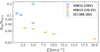 |
Fig. 4. Fit results for the iron abundances of MBO2, MBO3, and DI1388 as a function of different microturbulence values ξ. |
By combining the posterior distributions for the different fixed ξ as described in Appendix B, we obtained a final iron mass fraction of 
 for MBO2 and
 for MBO3. These values are lower than the adopted Fe abundance in the Ramachandran et al. (2021) models, but they are not different enough to affect the line predictions of other elements in the optical range. Based on the unaffected main stellar parameters and C, N, O, Mg, and Si abundances, we can thus combine our results with the abundances from Ramachandran et al. (2021) and our Ne assumption (see Sect. 3.3) to obtain a metallicity of 6.26 × 10⁻⁴ (∼4.75% Z⊙) for MBO2 and 1.10 × 10⁻³ (∼8.23% Z⊙) for MBO3. The derived flux shift values are within 5−7 × 10⁻¹⁵ erg cm−2 s−1 Å−1, which corresponds to a shift of about 4–8% of the measured UV flux and is in the same range as the measured flux uncertainties. A model-independent direct comparison of the Fe lines between S3 in Sextans A (Telford et al. 2024) and MBO2 suggests a similar or lower Fe content for MBO2 (see Appendix C).
4.2. Comparison with the B star DI 1388
To search for systematic differences with the metal-poor B star study by Dufton et al. (2008), we analyzed DI 1388. We adopted the same stellar and broadening parameters from Hambly et al. (1994) as were used by Dufton et al. (2008). We calculated a grid of models for DI 1388 with varying Fe abundances and a fixed microturbulence of ξ = 5 km s−1. Instead of the plane-parallel TLUSTY code (Hubeny 1988), we used the spherically symmetric PoWR models and the same fitting procedure as described above to derive the iron abundances.
In comparison to Dufton et al. (2008, XFe = 1.26% XFe, ⊙), we determined a much higher iron abundance of XFe = (21 ± 1)% XFe, ⊙ which is in the range of the mean SMC metallicity. The comparison of the best-fit model with the data is shown in Fig. E.12, and the corresponding corner plot is shown in Fig. E.11. The difference in the derived Fe abundance arises from a combination of factors that includes the differences in the i) underlying models, ii) the fitting methods, and iii) the observational data. A major factor for the differences may be the different considered spectral wavelength ranges in Dufton et al. (2008) in comparison to this work. In contrast to Dufton et al. (2008), who used the range of 1890−1930 Å that mainly covers the Fe III forest lines, we fit the models to the observed spectral range that covers both the Fe IV and Fe V forest (see, e.g., Hillier 2020). At a temperature of ∼32 kK, Fe IV and Fe V are the dominant ions. The spectral range we chose is therefore more suitable. Additionally, the HST-GHRS spectra have a much lower signal-to-noise ratio (S/N = 3) than the STIS spectra (S/N = 10 − 25) we used.
4.3. Abundance patterns and signs of an α enhancement
Our derived Fe abundances of O stars along with the light metal abundances estimated from optical spectra (Ramachandran et al. 2021) suggest that the O stars exhibit distinct chemical abundances despite their close spatial proximity (projected distance of ∼15 pc). A summary of the different metallicity measures of the analyzed stars can be found in Table 1. MBO2 and MBO3 are both significantly metal deficient by more than a factor of two than the average ISM metallicity reported by Lehner et al. (2008). In contrast, the more distant B star DI 1388 (projected distance ∼3.3 kpc) exhibits SMC-like Fe and overall elemental abundances. An important result is that the iron abundances of MBO2 and MBO3 do not scale with the abundances of oxygen and other light elements. Although it has the lowest mean abundance of light metals of Δ[X/H] = −1.35, MBO2 has a higher fraction of iron, [Fe/H] = −0.97. In contrast, MBO3 has a higher mean abundance of light metals of Δ[X/H] = −0.98, but a significantly lower iron content of [Fe/H] = −1.44.
Comparison of the abundance measurements of hot massive stars and the ISM in the Magellanic Bridge.
Figure 5 shows the X/Fe ratios (relative to solar values) for each element, including alpha elements such as O, Mg, and Si. This illustrates how the elemental abundances scale with iron. While α-elements are mainly produced in massive stars and are distributed to the ISM via their core-collapse supernovae, iron is primarily produced with a time delay through type Ia supernovae. MBO3, which has the lowest iron content, shows signs for a significant α-enhancement. In MBO2, O and Si are depleted relative to Fe, whereas Mg exhibits a slight enhancement.
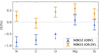 |
Fig. 5. Depletion of metals relative to iron. Only an upper limit was determined for the oxygen abundance of MBO2 (Ramachandran et al. 2021). This is highlighted by an arrow. |
Thus, our analysis further confirms the inhomogeneous ISM of the Magellanic Bridge that was suggested by Ramachandran et al. (2021) based on light element abundances. We find a large scatter in the Fe abundances (∼20 − 3% Z⊙) and distinct [α/Fe] ratios. These inhomogeneities may be linked to multiple gas-accretion epochs, tidal interactions, or localized enrichment processes. To fully understand the complex chemical evolution of the Bridge, a more detailed and systematic chemical abundance analysis of a larger sample of young stars throughout the Bridge is essential (Schösser et al., in prep.).
5. Conclusions
The low iron content of the stars and the inhomogeneities in their individual elemental abundances make the discovered O stars in the Magellanic Bridge unique counterparts to the high-z Universe, where similar conditions likely existed. Our results suggest that inhomogeneous mixing occurs even at the current epoch. At earlier times, mixing would have been even less efficient. Thus, great caution is required when the abundances from integrated populations at high z are determined and interpreted. A variety of abundances is observed already within the SMC and its outskirts. This variety is most likely driven by interactions. At high z, these interactions were likely even more frequent and continuously changed the chemical content of the environment. Moreover, our results highlight that there is no simple scaling between oxygen and iron even for young stars, and the inference from one element to the next can lead to significant over- or underestimations. Iron is the main driver for winds, and it thus defines the main physics of the stars. These inaccuracies can therefore have severe consequences for the inferred stellar evolution. This in turn leads to uncertainties in spectral energy distributions and ionizing radiation that affect the chemical abundances that are derived from H II regions and contributions to cosmic reionization.
Acknowledgments
ECS acknowledges financial support by the Federal Ministry for Economic Affairs and Climate Action (BMWK) via the German Aerospace Center (Deutsches Zentrum für Luft- und Raumfahrt, DLR) grant 50 OR 2306 (PI: Ramachandran/Sander) and by the Federal Ministry of Education and Research (BMBF) and the Baden-Württemberg Ministry of Science as part of the Excellence Strategy of the German Federal and State Governments. ECS, VR, AACS, MBP, and RRL acknowledge support by the German Deutsche Forschungsgemeinschaft, DFG in the form of an Emmy Noether Research Group – Project-ID 445674056 (SA4064/1-1, PI Sander). GGT acknowledges financial support by the Federal Ministry for Economic Affairs and Climate Action (BMWK) via the German Aerospace Center (Deutsches Zentrum für Luft- und Raumfahrt, DLR) grant 50 OR 2503 (PI: Sander). GGT and JJ further acknowledge funding from the Deutsche Forschungsgemeinschaft (DFG, German Research Foundation) Project-ID 496854903 (SA4064/2-1, PI Sander).
References
- Abbott, D. C. 1982, ApJ, 259, 282 [Google Scholar]
- Asplund, M., Grevesse, N., Sauval, A. J., & Scott, P. 2009, ARA&A, 47, 481 [NASA ADS] [CrossRef] [Google Scholar]
- Backs, F., Brands, S. A., de Koter, A., et al. 2024, A&A, 692, A88 [NASA ADS] [CrossRef] [EDP Sciences] [Google Scholar]
- Bernini-Peron, M., Sander, A. A. C., Ramachandran, V., et al. 2024, A&A, 692, A89 [NASA ADS] [CrossRef] [EDP Sciences] [Google Scholar]
- Bouret, J. C., Lanz, T., Hillier, D. J., et al. 2003, ApJ, 595, 1182 [NASA ADS] [CrossRef] [Google Scholar]
- Bouret, J. C., Lanz, T., Hillier, D. J., et al. 2015, MNRAS, 449, 1545 [NASA ADS] [CrossRef] [Google Scholar]
- Boyett, K., Bunker, A. J., Curtis-Lake, E., et al. 2024, MNRAS, 535, 1796 [NASA ADS] [CrossRef] [Google Scholar]
- Bromm, V., Coppi, P. S., & Larson, R. B. 2002, ApJ, 564, 23 [Google Scholar]
- Chiosi, C., & Maeder, A. 1986, ARA&A, 24, 329 [NASA ADS] [CrossRef] [Google Scholar]
- Cohen, J. G., Christlieb, N., McWilliam, A., et al. 2008, ApJ, 672, 320 [NASA ADS] [CrossRef] [Google Scholar]
- Curti, M., Maiolino, R., Curtis-Lake, E., et al. 2024, A&A, 684, A75 [NASA ADS] [CrossRef] [EDP Sciences] [Google Scholar]
- Dufton, P. L., Ryans, R. S. I., Thompson, H. M. A., & Street, R. A. 2008, MNRAS, 385, 2261 [NASA ADS] [CrossRef] [Google Scholar]
- Evans, C. J., Castro, N., Gonzalez, O. A., et al. 2019, A&A, 622, A129 [NASA ADS] [CrossRef] [EDP Sciences] [Google Scholar]
- Foreman-Mackey, D., Hogg, D. W., Lang, D., & Goodman, J. 2013, PASP, 125, 306 [Google Scholar]
- Garcia, M., Herrero, A., Najarro, F., Lennon, D. J., & Alejandro Urbaneja, M. 2014, ApJ, 788, 64 [NASA ADS] [CrossRef] [Google Scholar]
- Garcia, M., Herrero, A., Najarro, F., Camacho, I., & Lorenzo, M. 2019, MNRAS, 484, 422 [Google Scholar]
- Garg, P., Narayanan, D., Sanders, R. L., et al. 2024, ApJ, 972, 113 [NASA ADS] [CrossRef] [Google Scholar]
- Gräfener, G., Koesterke, L., & Hamann, W. R. 2002, A&A, 387, 244 [NASA ADS] [CrossRef] [EDP Sciences] [Google Scholar]
- Gratton, R. G., & Sneden, C. 1988, A&A, 204, 193 [NASA ADS] [Google Scholar]
- Green, J. C., Froning, C. S., Osterman, S., et al. 2012, ApJ, 744, 60 [NASA ADS] [CrossRef] [Google Scholar]
- Hamann, W. R., & Gräfener, G. 2003, A&A, 410, 993 [CrossRef] [EDP Sciences] [Google Scholar]
- Hambly, N. C., Dufton, P. L., Keenan, F. P., et al. 1994, A&A, 285, 716 [Google Scholar]
- HI4PI Collaboration (Ben Bekhti, N., et al.) 2016, A&A, 594, A116 [NASA ADS] [CrossRef] [EDP Sciences] [Google Scholar]
- Hillier, D. J. 2020, Galaxies, 8, 60 [NASA ADS] [CrossRef] [Google Scholar]
- Hindman, J. V., Kerr, F. J., & McGee, R. X. 1963, Aust. J. Phys., 16, 570 [Google Scholar]
- Hopkins, P. F., Wetzel, A., Wheeler, C., et al. 2023, MNRAS, 519, 3154 [Google Scholar]
- Hubeny, I. 1988, Comput. Phys. Commun., 52, 103 [Google Scholar]
- Jacyszyn-Dobrzeniecka, A. M., Skowron, D. M., Mróz, P., et al. 2016, Acta Astron., 66, 149 [NASA ADS] [Google Scholar]
- Janka, H. T., Langanke, K., Marek, A., Martínez-Pinedo, G., & Müller, B. 2007, Phys. Rep., 442, 38 [NASA ADS] [CrossRef] [Google Scholar]
- Johnson, C. I., Plesha, R., Jedrzejewski, R., Frazer, E., & Dashtamirova, D. 2021, Updated Flux Error Calculations for CalCOS, Instrument Science Report COS 2021-03 [Google Scholar]
- Laseter, I. H., Maseda, M. V., Curti, M., et al. 2024, A&A, 681, A70 [NASA ADS] [CrossRef] [EDP Sciences] [Google Scholar]
- Lehner, N., Sembach, K. R., Dufton, P. L., Rolleston, W. R. J., & Keenan, F. P. 2001, ApJ, 551, 781 [NASA ADS] [CrossRef] [Google Scholar]
- Lehner, N., Howk, J. C., Keenan, F. P., & Smoker, J. V. 2008, ApJ, 678, 219 [NASA ADS] [CrossRef] [Google Scholar]
- Matthee, J., Mackenzie, R., Simcoe, R. A., et al. 2023, ApJ, 950, 67 [NASA ADS] [CrossRef] [Google Scholar]
- Pauldrach, A. 1987, A&A, 183, 295 [NASA ADS] [Google Scholar]
- Ramachandran, V., Hamann, W. R., Oskinova, L. M., et al. 2019, A&A, 625, A104 [NASA ADS] [CrossRef] [EDP Sciences] [Google Scholar]
- Ramachandran, V., Oskinova, L. M., & Hamann, W. R. 2021, A&A, 646, A16 [NASA ADS] [CrossRef] [EDP Sciences] [Google Scholar]
- Rickard, M. J., Hainich, R., Hamann, W. R., et al. 2022, A&A, 666, A189 [NASA ADS] [CrossRef] [EDP Sciences] [Google Scholar]
- Rolleston, W. R. J., Dufton, P. L., McErlean, N. D., & Venn, K. A. 1999, A&A, 348, 728 [NASA ADS] [Google Scholar]
- Rowland, L. E., Stefanon, M., Bouwens, R., et al. 2025, ArXiv e-prints [arXiv:2501.10559] [Google Scholar]
- Sander, A., Shenar, T., Hainich, R., et al. 2015, A&A, 577, A13 [NASA ADS] [CrossRef] [EDP Sciences] [Google Scholar]
- Scott, P., Asplund, M., Grevesse, N., Bergemann, M., & Sauval, A. J. 2015a, A&A, 573, A26 [NASA ADS] [CrossRef] [EDP Sciences] [Google Scholar]
- Scott, P., Grevesse, N., Asplund, M., et al. 2015b, A&A, 573, A25 [NASA ADS] [CrossRef] [EDP Sciences] [Google Scholar]
- Seaton, M. J. 1979, MNRAS, 187, 73 [Google Scholar]
- Telford, O. G., Chisholm, J., Sander, A. A. C., et al. 2024, ApJ, 974, 85 [NASA ADS] [Google Scholar]
- Urbaneja, M. A., Bresolin, F., & Kudritzki, R.-P. 2023, ApJ, 959, 52 [Google Scholar]
- Valerdi, M., Peimbert, A., Peimbert, M., & Sixtos, A. 2019, ApJ, 876, 98 [NASA ADS] [CrossRef] [Google Scholar]
- Vink, J. S., de Koter, A., & Lamers, H. J. G. L. M. 2001, A&A, 369, 574 [NASA ADS] [CrossRef] [EDP Sciences] [Google Scholar]
- Vink, J. S., Mehner, A., Crowther, P. A., et al. 2023, A&A, 675, A154 [NASA ADS] [CrossRef] [EDP Sciences] [Google Scholar]
- Woosley, S. E., Heger, A., & Weaver, T. A. 2002, Rev. Mod. Phys., 74, 1015 [NASA ADS] [CrossRef] [Google Scholar]
Appendix A: Data normalization and reduction
The UV spectra were obtained from Mikulski Archive for Space Telescopes (MAST) and are standard pipeline-processed data. We normalize the observed spectra (listed in Table A.1) by dividing them by a synthetic PoWR model continuum. As the shape of the spectral continuum does not change significantly for different iron metallicities between 1 and 15 %, we use a model with a fixed iron group mass fraction of 5% G⊙ to normalize the UV spectra. Additionally, we applied a small flux shift to the synthetic model continuum. These shifts remained consistent with measured photometry. For the Bayesian inference of the iron abundances (see Section 3.3), we treated this flux shift as a free parameter in our fitting process, as it is difficult to distinguish between the uncertainty level and the absorption lines. Thus, instead of normalizing the spectrum once, we repeat the process for all iterations during the Bayesian sampling process.
We then apply a radial velocity shift to the model spectra, 169 km s−1 and 163 km s−1 for MBO2 and MBO3 respectively. Furthermore, we account for galactic foreground and SMC reddening by applying the reddening law of Seaton (1979) with EB − V = 0.08 to all model spectra. Additionally, we convolve the model spectra with a Gaussian with FWHM = 0.1 to account for HST-COS’s instrumental broadening, with a half-ellipse to account for rotation, and with a radial-tangential profile to account for macroturbulence.
Details of the HST UV observations.
Appendix B: χ2 fit of the microturbulences
We quantify the goodness of the fit for different microturbulences by computing
 (B.1)
(B.1)
which is the squared difference between the observed and model spectra, divided by the flux uncertainty σi2 at the i-th wavelength point. As we did not vary the sulfur abundance and we are only interested in the fit of the wings, we only compute χ2 for the wing region of the S V line which we define by a velocity shift between 10 and 60 km s−1 around the center of the line (see Fig. 2). The computed χ2 values for models with different ξ for MBO2 and MBO3 are depicted in Fig. B.1.
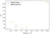 |
Fig. B.1. Computed χ2 values for the wavelength range corresponding to the shaded region in Fig. 2 as a function of micro-turbulence for MBO2 and MBO3. |
We derive the final iron abundances and associated uncertainties by considering the probability distribution of microturbulences. This is achieved by assigning normalized weights
 (B.2)
(B.2)
to each microturbulence where we use the χ2 value as derived from Equation (B.1). We combine the iron abundance posterior distributions as follows:
 (B.3)
(B.3)
Appendix C: Comparison with S3
As a model-independent comparison of the metal content, we compare the UV spectrum of MBO2 with the star S3 in Sextans A in Fig. C.1, which have the same spectral type. To account for the significantly higher rotation of S3, we convolved the spectrum of MBO2 to match the observed v sin i = 200 km s−1 of S3. Despite the noise in the spectrum of S3, MBO2’s Fe lines appear similar to or weaker than those in S3, confirming the sub-SMC iron abundance of MBO2 and providing an independent consistency check of our new Fe abundance determination method.
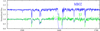 |
Fig. C.1. Comparison of the UV spectrum of MBO2 (blue) convolved with a rotational broadening profile (v sin i = 200km/s, matching S3) with the observed UV spectrum of S3 (green). The original, unbroadened MBO2 spectrum (shifted upward for clarity) is also displayed. |
Appendix D: Atomic data
In Table D.1, we list the number of levels and line transitions accounted for in the non-LTE atmosphere calculations with PoWR.
Overview of the number of levels and lines per ion handled in non-LTE in the calculated atmosphere models.
Appendix E: Detailed fit results
In the following, we present the detailed fit results for MBO2, MBO3 and DI1388 including the corner plots and the best-fit model spectra over the full spectral range of HST/COS-G160M. The wavelength regimes that are ignored in the Bayesian analysis are highlighted by grey bands. For MBO2, we show the individual fit results for the microturbulences ξ = 1, 2 and 5 km s−1 (Figures E.1–E.4), for MBO3 for ξ = 3, 5, 8, 10 and 20 km s−1 (Figures E.5–E.10), and for DI1388 for ξ = 5 km s−1 (Figures E.11–E.12).
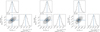 |
Fig. E.1. Corner plots for the fit of the iron mass fraction XFe and a flux shift in the spectral energy distribution for MBO2 and fixed microturbulence of ξ = 1 km s−1 (left), ξ = 2 km s−1 (middle) and ξ = 5 km s−1 (right). |
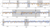 |
Fig. E.2. Comparison of the observed (dashed, blue line) and best-fit modelled spectrum (orange) for MBO2 and fixed microturbulence of ξ = 1 km s−1. The thick light blue line depicts a PP sample. Regions which are ignored in the fit are highlighted in grey. |
 |
Fig. E.3. Comparison of the observed (dashed, blue line) and best-fit modelled spectrum (orange) for MBO2 and fixed microturbulence of ξ = 2 km s−1. The thick light blue line depicts a PP sample. Regions which are ignored in the fit are highlighted in grey. |
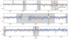 |
Fig. E.4. Comparison of the observed (dashed, blue line) and best-fit modelled spectrum (orange) for MBO2 and fixed microturbulence of ξ = 5 km s−1. The thick light blue line depicts a PP sample. Regions which are ignored in the fit are highlighted in grey. |
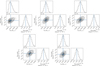 |
Fig. E.5. Corner plots for the fits of the iron mass fraction XFe and a flux shift in the spectral energy distribution for MBO3 and microturbulence of ξ = 3 km s−1 (upper left), ξ = 5 km s−1 (upper middle), ξ = 8 km s−1 (upper right), ξ = 10 km s−1 (lower left), and ξ = 20 km s−1 (lower right). |
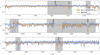 |
Fig. E.6. Comparison of the observed (dashed, blue line) and best-fit modelled spectrum (orange) for MBO3 and fixed microturbulence of ξ = 3 km s−1. The thick light blue line depicts a PP sample. Regions which are ignored in the fit are highlighted in grey. |
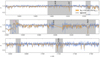 |
Fig. E.7. Comparison of the observed (dashed, blue line) and best-fit modelled spectrum (orange) for MBO3 and fixed microturbulence of ξ = 5 km s−1. The thick light blue line depicts a PP sample. Regions which are ignored in the fit are highlighted in grey. |
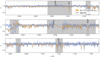 |
Fig. E.8. Comparison of the observed (dashed, blue line) and best-fit modelled spectrum (orange) for MBO3 and fixed microturbulence of ξ = 8 km s−1. The thick light blue line depicts a PP sample. Regions which are ignored in the fit are highlighted in grey. |
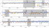 |
Fig. E.9. Comparison of the observed (dashed, blue line) and best-fit modelled spectrum (orange) for MBO3 and fixed microturbulence of ξ = 10 km s−1. The thick light blue line depicts a PP sample. Regions which are ignored in the fit are highlighted in grey. |
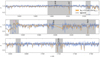 |
Fig. E.10. Comparison of the observed (dashed, blue line) and best-fit modelled spectrum (orange) for MBO3 and fixed microturbulence of ξ = 20 km s−1. The thick light blue line depicts a PP sample. Regions which are ignored in the fit are highlighted in grey. |
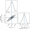 |
Fig. E.11. Corner plot for the fit of the iron mass fraction XFe and a flux shift in the spectral energy distribution for DI1388 and fixed microturbulence of ξ = 5 km s−1. |
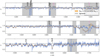 |
Fig. E.12. Comparison of the observed (dashed, blue line) and best-fit modelled spectrum (orange) for DI1388 and a fixed microturbulence of ξ = 5 km s−1. The thick light blue line depicts a PP sample. Regions which are ignored in the fit are highlighted in grey. |
All Tables
Comparison of the abundance measurements of hot massive stars and the ISM in the Magellanic Bridge.
Overview of the number of levels and lines per ion handled in non-LTE in the calculated atmosphere models.
All Figures
|
Fig. 1. Neutral hydrogen map of the Magellanic Clouds and the Magellanic Bridge from the HI4PI survey (HI4PI Collaboration 2016). The black plus marks the approximate position of MBO2 and MBO3 within the Magellanic Bridge, and the gray cross shows DI1388. |
| In the text | |
|
Fig. 2. Comparison of the observed and modeled S Vλ1501.76 line for different ξ for MBO2 (top) and MBO3 (bottom) in velocity space. The defined wing region in which we evaluated χ2 is highlighted. |
| In the text | |
|
Fig. 3. Comparison of the observed (dashed blue line) and best-fit modeled (orange) Fe IV forest of lines for fixed microturbulence values of ξ = 2 km s−1 for MBO2 (top) and ξ = 10 km s−1 for MBO3 (bottom). The thickness of the orange model line represents the 3σ credible interval of the best-fit model. A PP sample is shown in light blue. The full spectral fits are given in Appendix E. |
| In the text | |
|
Fig. 4. Fit results for the iron abundances of MBO2, MBO3, and DI1388 as a function of different microturbulence values ξ. |
| In the text | |
|
Fig. 5. Depletion of metals relative to iron. Only an upper limit was determined for the oxygen abundance of MBO2 (Ramachandran et al. 2021). This is highlighted by an arrow. |
| In the text | |
|
Fig. B.1. Computed χ2 values for the wavelength range corresponding to the shaded region in Fig. 2 as a function of micro-turbulence for MBO2 and MBO3. |
| In the text | |
|
Fig. C.1. Comparison of the UV spectrum of MBO2 (blue) convolved with a rotational broadening profile (v sin i = 200km/s, matching S3) with the observed UV spectrum of S3 (green). The original, unbroadened MBO2 spectrum (shifted upward for clarity) is also displayed. |
| In the text | |
|
Fig. E.1. Corner plots for the fit of the iron mass fraction XFe and a flux shift in the spectral energy distribution for MBO2 and fixed microturbulence of ξ = 1 km s−1 (left), ξ = 2 km s−1 (middle) and ξ = 5 km s−1 (right). |
| In the text | |
|
Fig. E.2. Comparison of the observed (dashed, blue line) and best-fit modelled spectrum (orange) for MBO2 and fixed microturbulence of ξ = 1 km s−1. The thick light blue line depicts a PP sample. Regions which are ignored in the fit are highlighted in grey. |
| In the text | |
|
Fig. E.3. Comparison of the observed (dashed, blue line) and best-fit modelled spectrum (orange) for MBO2 and fixed microturbulence of ξ = 2 km s−1. The thick light blue line depicts a PP sample. Regions which are ignored in the fit are highlighted in grey. |
| In the text | |
|
Fig. E.4. Comparison of the observed (dashed, blue line) and best-fit modelled spectrum (orange) for MBO2 and fixed microturbulence of ξ = 5 km s−1. The thick light blue line depicts a PP sample. Regions which are ignored in the fit are highlighted in grey. |
| In the text | |
|
Fig. E.5. Corner plots for the fits of the iron mass fraction XFe and a flux shift in the spectral energy distribution for MBO3 and microturbulence of ξ = 3 km s−1 (upper left), ξ = 5 km s−1 (upper middle), ξ = 8 km s−1 (upper right), ξ = 10 km s−1 (lower left), and ξ = 20 km s−1 (lower right). |
| In the text | |
|
Fig. E.6. Comparison of the observed (dashed, blue line) and best-fit modelled spectrum (orange) for MBO3 and fixed microturbulence of ξ = 3 km s−1. The thick light blue line depicts a PP sample. Regions which are ignored in the fit are highlighted in grey. |
| In the text | |
|
Fig. E.7. Comparison of the observed (dashed, blue line) and best-fit modelled spectrum (orange) for MBO3 and fixed microturbulence of ξ = 5 km s−1. The thick light blue line depicts a PP sample. Regions which are ignored in the fit are highlighted in grey. |
| In the text | |
|
Fig. E.8. Comparison of the observed (dashed, blue line) and best-fit modelled spectrum (orange) for MBO3 and fixed microturbulence of ξ = 8 km s−1. The thick light blue line depicts a PP sample. Regions which are ignored in the fit are highlighted in grey. |
| In the text | |
|
Fig. E.9. Comparison of the observed (dashed, blue line) and best-fit modelled spectrum (orange) for MBO3 and fixed microturbulence of ξ = 10 km s−1. The thick light blue line depicts a PP sample. Regions which are ignored in the fit are highlighted in grey. |
| In the text | |
|
Fig. E.10. Comparison of the observed (dashed, blue line) and best-fit modelled spectrum (orange) for MBO3 and fixed microturbulence of ξ = 20 km s−1. The thick light blue line depicts a PP sample. Regions which are ignored in the fit are highlighted in grey. |
| In the text | |
|
Fig. E.11. Corner plot for the fit of the iron mass fraction XFe and a flux shift in the spectral energy distribution for DI1388 and fixed microturbulence of ξ = 5 km s−1. |
| In the text | |
|
Fig. E.12. Comparison of the observed (dashed, blue line) and best-fit modelled spectrum (orange) for DI1388 and a fixed microturbulence of ξ = 5 km s−1. The thick light blue line depicts a PP sample. Regions which are ignored in the fit are highlighted in grey. |
| In the text | |
Current usage metrics show cumulative count of Article Views (full-text article views including HTML views, PDF and ePub downloads, according to the available data) and Abstracts Views on Vision4Press platform.
Data correspond to usage on the plateform after 2015. The current usage metrics is available 48-96 hours after online publication and is updated daily on week days.
Initial download of the metrics may take a while.