| Issue |
A&A
Volume 696, April 2025
|
|
|---|---|---|
| Article Number | A196 | |
| Number of page(s) | 15 | |
| Section | Catalogs and data | |
| DOI | https://doi.org/10.1051/0004-6361/202453624 | |
| Published online | 25 April 2025 | |
SED Modelling of Young Stellar Objects in the Orion Star Formation Complex
1
Konkoly Observatory, Research Centre for Astronomy and Earth Sciences, Hungarian Research Network (HUN-REN),
1121 Budapest,
Konkoly Thege Miklós út 15–17,
Hungary
2
CSFK, MTA Centre of Excellence,
Budapest,
Konkoly Thege Miklós út 15–17,
1121,
Hungary
3
Department of Astronomy, University of Geneva,
Chemin Pegasi 51,
1290
Versoix, Switzerland
4
Department of Astrophysics, University of Vienna,
Türkenschanzstrasse 17,
1180
Vienna, Austria
5
Natural History Museum Vienna,
Burgring 7,
1010
Vienna, Austria
★ Corresponding author; This email address is being protected from spambots. You need JavaScript enabled to view it.
Received:
28
December
2024
Accepted:
25
February
2025
Abstract
Context. One of the key tools for understanding the evolution of young stellar objects (YSOs) is to analyse their spectral energy distributions (SEDs). As part of the NEMESIS project, we have performed a large-scale SED fitting analysis of the Orion star formation complex (OSFC).
Aims. We aim to derive key physical parameters, including temperature, luminosity, mass, and age, for a large sample of sources in the OSFC using synthetic SED models. Our goal is to establish a statistically robust characterisation of the stellar population and its evolutionary state across the entire complex.
Methods. We utilize a set of new radiative transfer model SEDs that span a variety of geometries and parameter spaces. These SEDs are fitted to multi-wavelength photometric data from optical to submillimeter wavelengths. We conducted SED fitting on a sample of 15 396 sources. Among these, 5062 have at least a reliable W3 (12 µm) detection at longer wavelengths, and 63 have sub-millimeter detections in APEX/SABOCA at 350 µm or APEX/LABOCA at 870 µm. The resulting physical parameters are cross-referenced with stellar evolutionary tracks to ensure consistency with theoretical predictions.
Results. The derived parameters reveal a diverse stellar population. Sources placed on the Hertzsprung-Russell diagram show distinct evolutionary sequences. The results are provided with varying levels of completeness and reliability, depending on the available data for each source. The catalogue includes quality indicators such as the flux code, which represents the longest detected wavelength for each source, as well as Prob_W3 and Prob_W4 values that quantify the reliability of the AllWISE W3 and W4 detections. All results, including SED fitting outcomes, uncertainty estimates, and source metadata, are publicly available in a comprehensive CDS table.
Conclusions. This dataset provides a statistically significant view of the evolutionary processes within the OSFC. The publicly accessible dataset offers a valuable resource for future studies on star and planet formation.
Key words: planets and satellites: formation / planets and satellites: general / stars: formation / stars: pre-main sequence / stars: protostars / stars: statistics
© The Authors 2025
 Open Access article, published by EDP Sciences, under the terms of the Creative Commons Attribution License (https://creativecommons.org/licenses/by/4.0), which permits unrestricted use, distribution, and reproduction in any medium, provided the original work is properly cited.
This article is published in open access under the Subscribe to Open model. This email address is being protected from spambots. You need JavaScript enabled to view it. to support open access publication.
1 Introduction
Star formation occurs in molecular clouds when a rotating, magnetised cloud collapses under its gravity. Despite this relatively simple description, the physical processes that govern star formation remain a significant area of active research in astronomy. Young stellar objects (YSOs) represent an early phase in stellar evolution, often associated with the surrounding gas and dust from which they form. These objects are frequently observed in regions of active star formation, such as stellar nurseries and molecular clouds. Among these regions, the Orion star formation complex (OSFC), located at a distance of approximately 400 parsecs (Menten et al. 2007; Groβschedl et al. 2018; Kuhn et al. 2019), is the closest major star-forming region and one of the most extensively studied. It provides critical insights into both low- and high-mass star formation, the evolution and dispersal of star-forming clouds, and the dynamics of the interstellar medium.
Research on YSOs has unveiled a variety of complex detection and characterisation methods across different scientific domains. Spectroscopic techniques, exemplified by Briceño et al. (2019), identified over 2000 T Tauri stars in Orion OB1 by analysing the Li I line absorption and Hα emission characteristics. Further expanding our understanding, Kounkel et al. (2018) conducted a kinematic analysis, detecting approximately 9000 kinematic members using Gaia DR2 (Gaia Collaboration 2018) positions, proper motions, and radial velocity data from the Apache Point Observatory Galactic Evolution Experiment (APOGEE; Majewski et al. 2017). Additionally, photometric variability research has uncovered multiple mechanisms influencing stellar observation, such as stellar rotation, magnetic spots, disc dust dimming, and fluctuations in the accretion rate (Morales-Calderón et al. 2011; Cody & Hillenbrand 2010; Cody et al. 2014; Cody & Hillenbrand 2018).
One of the key tools for understanding the evolutionary stages of YSOs is the spectral energy distribution (SED), which represents an object’s energy output across a wide range of the electromagnetic spectrum, from gamma rays to radio waves. By plotting flux as a function of wavelength, the shape of the SED reveals crucial information about the physical properties and evolutionary stages of YSOs. In their early stages, YSOs exhibit a significant infrared excess, primarily due to circumstellar discs and envelopes that reprocess stellar radiation into thermal emission. As these objects evolve, their SEDs gradually transition from being dominated by circumstellar material to resembling stellar photospheres, with a diminishing infrared excess. This evolution reflects the dissipation of circumstellar material as the star approaches the main sequence. Thus, analysing SED shapes is vital for understanding both the formation and early evolution of stars and planetary systems.
Young stellar objects are often classified into different evolutionary classes based on their infrared SEDs, with a spectral index α serving as a key parameter to differentiate between classes (Lada 1987; Adams et al. 1987; Andre & Montmerle 1994; Evans et al. 2009a; Dunham et al. 2014). The infrared spectral index a measures how the flux density, Fλ, changes with wavelength, λ, and is calculated using the equation,

In practice, α is computed by performing a linear fit to the SED in logarithmic space, allowing researchers to infer the evolutionary phases of YSOs based on their infrared emission characteristics.
Initially, three classes (Class I, II, III) were defined (Lada & Wilking 1984; Lada 1987) and later expanded to five (Class 0, I, Flat, II, III; Greene et al. 1994). Class 0 represents the earliest collapse phase, dominated by an envelope (Andre et al. 1993). Classes I, II, and III correspond to protostars, pre-main-sequence stars with circumstellar discs, and evolved pre-main-sequence stars or main-sequence stars, respectively. Flat-spectrum sources, which lie between Classes I and II, have an ambiguous evolutionary status due to geometric effects, extinction, and observational biases (Whitney et al. 2003b,a, 2013; Robitaille et al. 2006; Crapsi et al. 2008).
A common technique for inferring the physical properties of YSOs is SED fitting, which compares observed SEDs with theoretical models to derive parameters such as temperature, luminosity, and characteristics of the circumstellar matter. While this method may seem straightforward, accurately determining the properties of YSOs from SED models is challenging due to model limitations and observational uncertainties. Traditional model grids are often biased due to specific theoretical assumptions or limited parameter sampling. The models introduced by Robitaille (2017, hereafter R17) offer broader geometric diversity and random parameter sampling, enhancing their applicability. However, these models lack certain critical parameters, such as core mass, and can sometimes produce unphysical scenarios. To address these limitations, Richardson et al. (2024, hereafter R24) recently updated the R17 models to improve their physical realism and expand their utility.
In constructing comprehensive SEDs, flux measurements across a wide range of wavelengths are essential. For YSOs, the infrared excess – arising from heated dust – provides crucial information about circumstellar environments, but it can obscure the underlying stellar emission. As a result, accurate SED fitting is critical for disentangling the contributions of the star and its surrounding material.
The Novel Evolutionary Model for the Early Stages of Stars with Intelligent Systems (NEMESIS)1 project aims to revolutionise our understanding of star formation by leveraging artificial intelligence to analyse the largest panchromatic YSO dataset (see, e.g. Roquette et al. 2025; Marton et al. 2024; Hernandez et al. 2024; Madarász et al. 2025). In addition to compiling the largest YSO catalogue for the OSFC, NEMESIS enhances data quality through advanced machine learning and deep learning techniques (Marton et al. 2024; Madarász et al. 2025). As part of the NEMESIS project, we have undertaken an extensive review of existing catalogues and literature to compile the most comprehensive YSO catalogue for the OSFC, including a detailed review of data from the Wide-field Infrared Survey Explorer (WISE; Wright et al. 2010) and the Herschel Space Observatory (Pilbratt et al. 2010). The OSFC covers a field of view spanning 564 square degrees, between 74.2° < RA < 92° and –14.1° < Dec < 17.6°.
Our work includes 27 879 sources with detailed positional information, flux measurements, and associated uncertainties across multiple wavelengths (Roquette et al. 2025), and it represents the largest dataset to date to which SED fitting has been applied for the classification of YSOs and the derivation of stellar parameters. We employ the updated radiative transfer model SEDs from R17 and R24.
This paper is organised as follows: Section 2 provides an overview of the surveys and catalogues used in our analysis, along with statistical details on the photometric data. Section 3 outlines the updated R24 model and describes the SED fitting methodology. The results of the SED fitting analysis are presented in Section 4. Section 5 discusses the findings, and Section 6 summarises our conclusions.
2 Data
Our SED analysis incorporates data from multiple astronomical surveys and instruments, including Gaia DR3 (Gaia Collaboration 2023), 2MASS (Skrutskie et al. 2006), WISE (Wright et al. 2010), Spitzer/IRAC (Fazio et al. 2004), Spitzer/MIPS (Rieke et al. 2004), Herschel (Pilbratt et al. 2010), and the Atacama Pathfinder Experiment (APEX) (Stutz et al. 2013). Below, we summarise the contributions of each dataset and its relevance to this study.
2.1 Gaia DR3
Gaia is one of the primary datasets utilised in our YSO catalogue, providing optical photometric and astrometric data for the largest number of YSOs. Gaia conducts a full-sky survey, delivering observations in three photometric bands: G (0.58 µm), BP (0.50 µm), and RP (0.76 µm). Approximately 20000 sources in our catalogue have available Gaia photometry in all three bands.
In our OSFC catalogue, we used parallax data from the third data release of the Gaia mission (GaiaDR3, Gaia Collaboration 2023) to determine accurate distances. To ensure reliability, we applied a 3-sigma cutoff to filter out sources with uncertain parallax data, thus reducing the impact of measurement uncertainties and excluding outliers. This process identified 22 275 sources (out of 27 879) with reliable parallax measurements. Of these, approximately 17 500 sources fall within the distance range of 200 to 600 parsecs (Kounkel et al. 2018; Groβschedl et al. 2019), which approximately corresponds to the OSFC. For these 17 500 sources, we utilized the precise Gaia distance in further SED fitting. For the remaining sources, where Gaia’s distance measurements were less reliable, unavailable, or outside the 200–600 parsecs range, we continued SED fitting using an average OSFC distance of 400 parsecs.
Despite its high precision, Gaia’s distance estimates in starforming regions can be unreliable. Factors such as interstellar dust, gas, and the diffuse environment of OSFC can affect parallax accuracy. Additionally, YSOs are often surrounded by dense envelopes or discs, which obscure optical observations. Variability caused by dynamic accretion processes further complicates these measurements. A similar challenge has been discussed in the context of AGB stars by Andriantsaralaza et al. (2022). Given these limitations, we chose to retain all sources in our catalogue, including those with less reliable or absent distance measurements, rather than imposing stricter selection criteria. The methodology used for data compilation is detailed in Roquette et al. (2025). Further discussion of the SED fitting process is provided in Section 3.2.
2.2 2MASS
The Two Micron All-Sky Survey (2MASS) was a ground-based survey that mapped the entire sky in near-infrared wavelengths in the J (1.235 µm), H (1.662 µm), and Ks (2.159 µm) bands. The 2MASS Point Source catalogue (Skrutskie et al. 2006) provides near-infrared photometry for the majority, over 23 000 sources of our OSFC YSOs catalogue.
2.3 Spitzer space telescope
Up until the launch of the James Webb Space Telescope (JWST) (Gardner et al. 2006), Spitzer Space Telescope (Werner et al. 2004) was the most sensitive infrared telescope. While JWST is a highly advanced and extremely sensitive observatory, it is still relatively new, and its primary focus on targeted studies rather than large-scale surveys means that Spitzer continues to provide the most sensitive infrared data for a greater number of sources. The Spitzer enabled extensive exploration of YSOs within the Milky Way through its Infrared Array Camera (IRAC) and Multiband Imaging Photometer (MIPS). IRAC observed at 3.6, 4.5, 5.8, and 8.0 µm, while MIPS covered 24 µm (MIPS1) and 70 µm (MIPS2). These comprehensive surveys, including the Galactic Legacy Infrared Midplane Survey Extraordinaire (GLIMPSE; Benjamin et al. 2003) and the MIPS Galaxy (MIPSGAL) surveys have played a crucial role in examining numerous star-forming regions (e.g. Allen et al. 2004; Megeath et al. 2004, 2005; Gutermuth et al. 2009; Megeath et al. 2012; Povich et al. 2011; Dunham et al. 2015). In our OSFC catalogue, approximately 10000 sources have IRAC photometry, while 2500 sources have data at 24 µm from MIPS. No sources in the catalogue have photometry at 70 µm.
2.4 WISE
While Spitzer provides sensitive infrared data for a greater number of sources, it still does not offer full-sky coverage. In this context, the WISE survey (Wright et al. 2010) is crucial due to its comprehensive full-sky coverage. As WISE is the only fullsky near-to-mid infrared survey, it often provides the primary mid-infrared photometry for sources. For WISE W1 and WISE W2 data, we used the CatWISE2020 catalogue (Eisenhardt et al. 2020; Marocco et al. 2021). The CatWISE2020 catalogue is a comprehensive dataset containing positions, brightnesses, and motion measurements for over 1.89 billion sources, derived from WISE and NEOWISE (Mainzer et al. 2014) observations spanning from 2010 to 2018. It focuses on wavelengths at 3.4 µm (W1) and 4.6µm (W2), making it valuable for studying stars, galaxies, and other celestial objects. CatWISE2020 uses 8 years of WISE and NEOWISE data, compared to AllWISE, which is limited to 4 years. Additionally, CatWISE2020 employs the ‘crowdsource’ detection algorithm (Schlafly et al. 2019) which is more effective in dense regions, such as the Galactic plane, where source blending is common.
The WISE mission was designed primarily for studying infrared-bright galaxies, brown dwarfs, and near-Earth asteroids. Consequently, detecting YSOs or evolved stars embedded in diffuse environments can be problematic, and photometry, particularly in the WISE W3 and W4 bands (at 12 and 22 µm), can be less reliable. This issue has been explored in various studies (e.g. Koenig & Leisawitz 2014; Marton et al. 2019; Silverberg et al. 2018), which indicated that previous methods were overly aggressive in filtering out spurious WISE W3 and W4 band photometry. To address this issue, we have updated these methodologies and incorporated new machine-learning techniques. Details of these improvements and the revised AllWISE catalogue are presented in Roquette et al. (2025). The updated AllWISE catalogue now includes probabilities indicating the likelihood that W3 and W4 band detections are real. For the sources in the OSFC, we provide the reliability values labeled as Prob_W3 and Prob_W4 enhancing the robustness of the SED fitting analysis.
2.5 Herschel space observatory
Herschel Space Telescope Pilbratt et al. (2010) is another major cornerstone in infrared astronomy. With a 3.5-meter primary mirror, Herschel was a space telescope operated as an observatory and performed diverse observing programs aimed at varied scientific objectives. Therefore, it didn’t cover the full sky, and only ~8% of the sky was observed with Herschel. The Herschel Space Observatory, which conducted many scientific observation programs, provided a catalogue of point sources (Marton et al. 2017) at 70, 100, and 160 µm. As part of NEMESIS, this catalogue was improved (Marton et al. 2024; Madarász et al. 2025) using advanced deep learning methods to ensure high reliability and to filter out unreliable sources. The final updated catalogue, recently published by Marton et al. (2024), provides reliable far-infrared (FIR) photometry for thousands of objects. However, since Herschel was not a full-sky survey, its coverage is patchy, and only hundreds of YSOs in the OSFC have Herschel photometry.
2.6 APEX
To extend the SEDs into the sub-millimeter range, we have included data from the Atacama Pathfinder EXperiment (APEX, Stutz et al. 2013). APEX is a submillimeter telescope located on the Chajnantor Plateau in the Atacama Desert, Chile. Operating at a high altitude of 5100 meters, it is optimized for observing the universe at millimeter and submillimeter wavelengths, crucial for studying cold gas and dust in space, star formation, and distant galaxies. LABOCA (Large APEX Bolometer Camera) is one of the primary instruments on APEX. It operates at 870 µm (350 GHz), in the submillimeter range. SABOCA (Submillimeter APEX Bolometer Camera) is another bolometer camera on APEX. It operates at a shorter wavelength of 350 µm (850 GHz), compared to LABOCA. For a few hundred sources, we have APEX/SABOCA data at 350µm and APEX/LABOCA data at 870 µm available.
Flux code abbreviations.
2.7 Photometric data compilation and data quality for SED fitting
We employed a total of 20 photometric filters for our study. The final dataset used for SED fitting includes flux measurements and associated errors from GaiaDR3, 2MASS, IRAC, CatWISE, AllWISE, PACS, and APEX. A notable addition to this table is the flux_code column, which indicates the farthest detected flux (non-NaN value) for each source. This column was specifically created to provide insight into the longest-wavelength detection for each source, helping to better understand their observational properties. Each code corresponds to a specific filter, as detailed in Table 1. The flux codes follow a hierarchical naming system, where shorter wavelengths are labelled first (e.g. I1 for IRAC 3.6 µm), and longer wavelengths are progressively labelled according to the farthest detected flux.
Additionally, we introduced the Prob_W3 and Prob_W4 columns to assess the reliability of AllWISE W3 and W4 photometry, enabling us to verify whether these detections are genuine. Figure 1 displays the number of sources with available photometric data for each filter. We performed the SED fitting analysis for sources with at least four valid data points. Out of the total 27 879 sources, 24 747 meet this criterion, ensuring a robust dataset for the fitting process.
2.8 Multiplicity considerations
The multiplicity labels in our study are based on the main Orion YSO catalogue compiled by Roquette et al. (2025), which provides a comprehensive assessment of binarity and source contamination. The catalogue underwent rigorous cleaning procedures, incorporating literature-based searches and advanced techniques, including machine learning and deep learning methods, to identify and flag potential binaries. As a result, the final dataset used in our SED fitting analysis was already scientifically curated to exclude known binaries and ambiguous sources, ensuring a more reliable interpretation of the fitted models. However, we acknowledge that observational limitations remain, and some unresolved binaries may still be present in the catalogue.
3 Methods
3.1 SED models
One of the most effective methods for characterising YSOs, especially when they are unresolved, is by fitting their SEDs to
pre-computed grids of radiative transfer models. Various SED model grids have been developed for this purpose, including those by Robitaille et al. (2007), Furlan et al. (2016), Haworth et al. (2018) and Zhang & Tan (2018). However, these models often assume specific star formation theories, limiting their applicability for testing different star formation scenarios. To address these limitations, the SED models presented by R17 offer a comprehensive set of templates that are agnostic to accretion history and stellar evolution models. These models span various geometries and parameter spaces, making them versatile tools for determining YSO properties. Nonetheless, R17 models had certain limitations, such as the absence of core mass values and the inclusion of unrealistic physical models.
Recently, the R17 models have undergone significant enhancements by R24, improving their utility and accuracy in determining YSO properties. The SEDs have been convolved with filters from JWST (Gardner et al. 2006), Paranal (Sutherland et al. 2015), additional Herschel filters, and Atacama Large Millimeter Array (ALMA) (Wootten & Thompson 2009) bands 3 and 6. The infrared spectral index α has been calculated for all SEDs within each aperture, facilitating the classification of YSOs into observational classes based on their evolutionary states. R24 determined the spectral index α as the slope of the line in log-space connecting the flux measurements at 2 and 25 µm and defined the classes as below.
Class I: α ≥ 0.3
Flat: -0.3 ≤ α < 0.3
Class II: -1.6 ≤ α< –0.3
Class III: α < –1.6.
The R17 model, along with its updated version by R24, consists of multiple components, including the star, disc, infalling envelope, bipolar cavities, and ambient medium. These components are modelled with varying levels of complexity, ranging from as few as two parameters in the simplest models to as many as twelve in the most detailed configurations. The models span a wide range of evolutionary stages, from the youngest, most deeply embedded YSOs to pre-main-sequence/main-sequence stars with minimal or no surrounding disc. Table 2 summarises the available model sets in both R17 and the updated R24 model. The updated model explicitly includes the luminosity of the central source for each configuration, enabling checks of the model’s position on the Hertzsprung-Russell (H-R) diagram. In contrast to previous versions, where outer envelope radii were not included and inner radii were either expressed in terms of the variable Rsub or omitted, the updated model provides these parameters explicitly. Additionally, the updated model offers further quantities, such as core mass, average dust temperature, and circumstellar extinction Av, facilitating a more comprehensive characterisation of YSOs.
R24 also adopts a stagification scheme to classify YSOs, utilizing the definitions from Crapsi et al. (2008) and Evans et al. (2009b) as a foundation. This scheme categorizes YSOs into four distinct stages based on the characteristics of their envelopes and central temperatures:
Stage 0: The envelope mass (Menv) is greater than 0.1 M⊙, and the stellar temperature (T⋆) is less than 3000 K.
Stage I: The envelope mass (Menv) remains greater than 0.1 M⊙, but the stellar temperature (T⋆) exceeds 3000 K.
Stage II: The envelope mass (Menv) is less than 0.1 M⊙, and a disc is present.
Stage III: The object is a bare pre-main-sequence star, with neither an envelope nor a disc.
Class is used for the observed SED classification, while Stage refers to the physical configuration. This classifica- tion/stagification system provides a structured framework for analyzing YSOs, offering clear distinctions between different evolutionary stages based on observable physical properties.
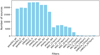 |
Fig. 1 Available flux counts for each filter. |
3.2 SED fitting
SED fitting involves comparing the observed SEDs of YSOs to a set of theoretical models that account for different physical components, such as the star, disc, infalling envelope, bipolar cavities, and ambient medium.
In our study of YSOs, we fit their SEDs using newly updated radiative transfer model SEDs from R24, utilizing the R17 SED fitting tool. Details of the R24 model are provided in the previous Section 3.1. In addition to several convolved filters of the R24 model, we have also added Gaia filters to the model. We have convolved the SEDs with filters from GaiaDR3 G, BP, and RP. The filter transmission curves were obtained from the SVO’s Filter Profile Service (Rodrigo et al. 2012; Rodrigo & Solano 2020).
As shown in Fig. 1, photometric data are not available for all sources across the 20 different bands. For our SED fitting analysis, we include all sources with at least four valid data points, regardless of whether they have detections at longer wavelengths. This inclusive approach is designed to minimise selection bias. Restricting sources to those with detections at longer wavelengths could exclude more evolved objects, which may no longer be detectable in these wavelength ranges.
SED fitting has been conducted for the 24 747 sources (see Section 2). For most of the sources, we used the optical Gaia G, BP and RP, 2MASS near-infrared (J, H, and Ks) photometry with mid-infrared photometry from either Spitzer/IRAC (3.6, 4.5, 5.8, and 8.0 µm) or/and WISE W1, W2 and W3 (3.4, 4.6, 12.0 µm). For a few thousand sources, we have been able to include Spitzer/MIPS at 24 µm or/and WISE W4 photometry at 22 µm. Only several hundred sources have far-infrared photometry from Herschel PACS and sub-millimeter data from APEX, and we have constructed SEDs for these sources ranging from optical to far-infrared (0.5 to 870 µm).
For sources with reliable Gaia distance measurements, we divided them into distance bins and performed individual fittings for each bin, allowing a 10% variation from the median distance. For sources where Gaia’s distance measurements were unreliable, unavailable, or fell outside the 200 to 600 parsecs range, we used a mean distance of 400 parsecs with a 10% variation.
We utilized the updated Galactic dust extinction estimates from Schlafly & Finkbeiner (2011), which were derived using the IRSA/IPAC Galactic Dust Map webpage2 in our analysis. Our findings indicate that 95% of the sources have extinction values ranging from 0 to 50 magnitudes. We accounted for interstellar extinction (AV) in the range of 0 to 50 mag, in addition to considering the extra extinction from the circumstellar environment of the YSOs. For this purpose, we applied the extinction law from Weingartner & Draine (2001) with a value of RV = 4.0.
To evaluate model fits, we used a Bayesian approach that assigns relative probabilities to models of varying complexity. We employed a threshold parameter (F = 3) to identify “good” fits. This selection follows the SED fitter model selection syntax, where ‘F’ indicates that we retain all models satisfying the condition that the reduced difference from the best-fit model, defined as  per datapoint, is below the chosen threshold value of 3. This ensures that we consider models that provide a statistically reasonable fit while excluding those with significantly higher deviations from the best-fit solution. This method helps avoid overfitting, particularly for sources with limited data points.
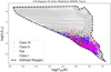 |
Fig. 2 Luminosity (L) as a function of effective temperature (Teff) is presented. Values are derived from the SED fitting of 15 396 best-fit models and overlaid on the PARSEC evolutionary tracks (with solar metallicity). The data points are colour-coded to represent different stellar classes. |
4 Results
We performed SED fitting for a total of 24747 sources. The updated model set was constructed to provide uniform coverage of the parameter space; however, some models remain nonphysical. To ensure the inclusion of only physically plausible models, we compared their positions on the H-R diagram with PAdova and TRieste Stellar Evolution Code (PARSEC; Bressan et al. 2012; Chen et al. 2014, 2015; Tang et al. 2014) evolutionary tracks. Based on this selection criterion, we successfully identified best-fit models for 15 396 sources (see Fig. 2). Table 2 summarises the model sets and their components, as described in R17, along with the number of sources matched to each set.
In Fig. 2, we present the temperature and luminosity of each source derived from the best-fit parameters on the H-R diagram, overlaid with evolutionary models from the PARSEC tracks. The PARSEC evolutionary tracks are theoretical models describing stellar evolution, computed using the PARSEC code, a widely adopted tool in stellar astrophysics. This release introduces a new implementation of pre-main sequence (PMS) evolution. During this phase, the star is fully convective, homogeneously mixed, and lacks active nuclear reactions. From this initial configuration, the star evolves at constant mass, progressing through the PMS contraction phase and subsequent stages of stellar evolution. Consequently, these tracks typically begin before the Zero-Age Main Sequence (ZAMS) for most stellar masses, spanning a range of 0.1–350 M⊙ (Bressan et al. 2012; Chen et al. 2015). The ZAMS marks the point where stellar models traditionally begin, as the physics in this phase is more stable and simpler compared to the complex processes of the PMS phase. Since our OSFC catalogue contains sources younger than the ZAMS, it is particularly advantageous to utilize the PARSEC tracks for our analysis.
Among the approximately 15 400 best-fit models, about 8950 correspond to sources with AllWISE W3 detections. However, as noted earlier, AllWISE W3 and W4 detections are not always reliable. To address this, we present a subset of more reliable SED fitting results for sources with robust detections. Specifically, we selected sources with a W3 (12 µm) detection at longer wavelengths and a detection probability (Prob_W3) greater than 50%. This criterion identifies a total of 5062 sources, referred to as the high-confidence subset.
Using the PARSEC evolutionary tracks, we estimated the mass and age of approximately 15 400 best-fit models. Stellar masses were determined by identifying the nearest evolutionary track, while stellar ages were interpolated from the closest point on the track corresponding to each source’s position in the H-R diagram.
For approximately 15 400 sources with successful fits, the complete results are available in the CDS table. This comprehensive dataset includes crucial SED fitting information such as flux_code indicating the longest wavelength detection for each source, along with the reliability probabilities for the AllWISE W3 and W4 photometry, Prob_W3 and Prob_W4, the number of valid data points used (ndpt), χ2 per data point for the best-fit model (χ2 per ndpt), and the number of fits (nfits) with χ2/ndpt between (χ2/ndpt)set and (χ2/ndpt)set + 2 within the most likely model set. Additionally, the table provides physical parameters estimated from the SED fitting - such as temperature and luminosity – alongside calculated values for Class, Stage, and spectral index.
We found that best-fit models incorporating Gaia data are relatively few, and their inclusion does not significantly improve the best-fit determination. In cases where Gaia data is available, the fitting process tends to favour models with circumstellar material (e.g. discs or envelopes), even for sources lacking detections beyond AllWISE W3 (12 µm). This effect arises because Gaia strongly constrains the optical brightness, whereas no equivalent constraint exists in the infrared. Consequently, the fitter may interpret any missing flux as being absorbed by circumstellar dust rather than interstellar extinction. Furthermore, chi-squared values were consistently higher when Gaia data was used, indicating that its inclusion does not always lead to a statistically better fit.
The Table A.1 in Appendix A presents the SED fitting results for a sample of 20 YSOs. The corresponding SED plots are also presented in Fig. A.1 in Appendix A. The table highlights key parameters used in SED fitting, providing critical insights into the reliability and limitations of the fitting process. The inclusion of ndpt highlights the diversity in data completeness across the sample, which directly impacts the robustness of the SED fitting. Sources with a higher number of data points provide more constrained fits, whereas sources with fewer data points may result in greater uncertainties. Similarly, the flux_code and detection probabilities (Prob_W3, Prob_W4) serve as indicators of the quality and reliability of individual photometric measurements. For instance, higher probabilities signify confident detections, enhancing the reliability of flux contributions at those wavelengths. Conversely, lower probabilities or missing values introduce additional uncertainties in the modelfitting process. Accurate distances are critical for determining the intrinsic physical properties of YSOs. For sources without precise parallax measurements, we adopt the average distance to the OSFC (400 pc). While this assumption is necessary for some sources, it introduces a degree of systematic uncertainty in the derived parameters. Together, these data for the 20 selected sources provide essential context for understanding the reliability and limitations of the SED fitting, enabling a more informed interpretation of the results.
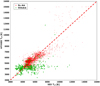 |
Fig. 3 Effective temperature (Teff) values from Kounkel et al. (2018) versus the Teff values derived from the SED fitting of 3482 high- confidence sources. Sources, where the best fitting model includes a disc, are plotted with green dots. |
5 Discussion
5.1 Comparison with the results of Kounkel et al. (2018)
Kounkel et al. (2018) provided key stellar properties, including effective temperature (Teff), surface gravity (log g), and radial velocity (RV), derived from the APOGEE spectra (Majewski et al. 2017) for approximately 9000 stars in the OSFC. Among the 15 396 successful best fits from our analysis, 6551 sources match those in the list provided by Kounkel et al. (2018). Furthermore, when we focus on the SED fitting results of high- confidence sources, 3482 of them match the list from Kounkel et al. (2018).
In Figure 3, we compare the effective temperature (Teff) values derived from the SED fitting of our high-confidence sources with those obtained by Kounkel et al. (2018) using APOGEE spectra. Despite the methodological differences in deriving these temperatures, the two sets of values show general agreement, and align well with those derived from APOGEE spectra, with a calculated Pearson’s correlation coefficient of 0.76. However, we note that sources with a disc component (green points in Figure 3) tend to show larger scatter, with many appearing along a horizontal distribution. This is likely due to the presence of circumstellar material contributing significant infrared excess, which can introduce degeneracies in the SED-based temperature determination. In particular, embedded or accreting sources may have their stellar photosphere partially veiled by disc emission, leading to systematic differences in the inferred Teff compared to spectroscopic estimates.
To assess the impact of circumstellar discs, we computed the correlation coefficient separately for sources with and without a disc component. When excluding disc-bearing sources, Pearson’s correlation coefficient improves to 0.82, suggesting that the SED-derived temperatures are more reliable in cases where the photospheric emission dominates.
5.2 Colour-colour diagrams
The identification and classification of YSOs in the OSFC have been extensively studied, particularly using colour-colour diagrams (e.g. Megeath et al. 2004, 2005; Gutermuth et al. 2009; Megeath et al. 2012, 2016). With the advent of Spitzer, these classifications were further tested. Several colour-colour diagrams were defined to distinguish different classes of YSOs (Megeath et al. 2004, 2005; Gutermuth et al. 2009), such as J–H vs. H–[4.5], and H–K vs. K-[4.5]. Megeath et al. (2004) and Allen et al. (2004) demonstrated that the IRAC colour-colour diagram ([3.6]–[4.5] vs. [5.8]-[8.0]) is a valuable tool for identifying young stars with infrared excess emission. Building on this, Muzerolle et al. (2004) combined MIPS 24 µm photometry with IRAC photometry and showed that the identified classes were almost entirely consistent with those identified using the [3.6][4.5] vs. [5.8]–[8.0] diagram, providing additional validation of this classification method.
Using Gaia BP, G, RP, 2MASS J, H, Ks, Spitzer/IRAC [3.6], [4.5], [5.8], [8.0], Spitzer/MIPS [24], [70], and WISE W1, W2, W3, and W4 magnitudes for our 5062 high-confidence sources, we have generated all possible colour-colour diagrams. In Fig. 4 we present the most commonly used colour-colour diagrams for the 5062 high-confidence sources. These sources have at least a W3 (12 µm) detection at longer wavelengths, with a detection probability (Prob_W3) greater than 50%. This threshold ensures that the W3 detection is both robust and reliable. As illustrated in the colour-colour diagrams, the separation between classes is well-defined, further underscoring the reliability of the SED fitting results when based on a comprehensive and accurate dataset.
5.3 Analysis of classification methods for YSOs
The updated R24 model introduces two complementary classification systems, as detailed in Section 3.1. The Class designation is based on the shape of the SED, while the Stage classification corresponds to the physical evolutionary phases of YSOs. Although the updated R24 model provides both class and stage definitions, we intentionally avoided comparing two systems derived from the same model. Instead, to perform an independent validation, we compared our SED-derived stages with classes determined by Hernandez et al. (2024).
Hernandez et al. (2024) introduces a novel approach to YSO classification within the NEMESIS project, which integrates two-dimensional (2D) morphological data alongside traditional infrared spectral index (αĮR) classification. These classifications are derived by associating source morphologies obtained using Self-Organizing Maps (SOMs). As a baseline for this study, Hernandez et al. (2024) adopts the infrared spectral index (αĮR) to classify YSOs based on the shape of their SEDs between 2–24 µm. This classification is performed using ordinary nonlinear least-squares fitting.
The classification scheme used in Hernandez et al. (2024) follows the framework established by Groβschedl et al. (2019), which is based on the observational classes originally defined by Lada (1987) and also adopted by R24 in their classification, as given in Equation (5.3). The only distinction from the R24 classification is that Hernandez et al. (2024) further subdivides the Class III phase into two groups: those with a disc and those without a disc. The classification scheme used by Hernandez et al. (2024) is as follows:
0/I: α ≥ 0.3
Flat: –0.3 ≤ a < 0.3
II: –1.6 ≤ α< –0.3
III thin disc: –2.5 ≤ a < –1.6
III no disc/MS: –2.5 ≥ α.
In Fig. 5, we present the distribution of sources across different combinations of SED-derived Stage classifications and the Class assignments from Hernandez et al. (2024). It is often assumed that the Class and Stage classification systems are aligned, with Class 0/I corresponding to Stage 0, Flat to Stage I, Class II to Stage II, and Class III thin disc and Class III no disc/MS to Stage III, representing equivalent evolutionary phases.
Fig. 5 reveals a strong correlation between Class III no disc/MS and Class III thin disc with Stage III, as well as between Flat and Stage II. This observed alignment suggests that the Class-based and Stage-based classifications exhibit a high degree of consistency, particularly in more evolved phases such as Stage III and Class III no disc/MS.
The relationship between these two classification systems indicates that the Stage classification effectively captures the physical evolution of YSOs, while the Class classification reflects observable characteristics, such as disc structure and envelope material. This alignment underscores the utility of both classification frameworks for tracking YSO evolution, with the Stage classification providing insights into physical processes and the Class classification highlighting observable features.
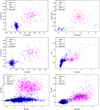 |
Fig. 4 Colour-colour diagrams for 5062 high-confidence sources, with classes derived from SED fitting. |
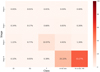 |
Fig. 5 Heatmap showing the distribution of stellar sources across different Stage and Class categories. Stages are derived from SED fitting, while Classes are adopted from Hernandez et al. (2024), providing a visual representation of the relationship between stellar evolutionary stages and classifications. |
5.4 Analysis of evolutionary trends in the OSFC
Circumstellar discs are critical structures in the star formation process, originating from the conservation of angular momentum during the collapse of molecular clouds. Advances in high- resolution instruments, such as ALMA (Wootten & Thompson 2009), have enabled detailed studies of these discs, revealing features such as Keplerian rotation and ring-like substructures (Tobin et al. 2016; Tychoniec et al. 2018; Tobin et al. 2020). These features are believed to play a pivotal role in early dust evolution and planet formation.
Theoretical models of disc formation integrate advanced physical processes, such as non-ideal magnetohydrodynamics, turbulence, and radiation transfer (Zhao et al. 2020; Manara et al. 2018, 2023; Yen & Lee 2024). Bridging these theoretical advancements with high-resolution observational data is essential for a comprehensive understanding of star and disc formation. While the debate about whether discs can form early in the star formation process may be resolved, the properties of actual protostellar discs remain critical for constraining these simulations.
Disc parameters, such as disc mass, cannot be well constrained without detections in the sub-mm; mid-infrared fluxes only provide a lower limit on the disc mass (R17). However, given that our catalogue provides large number of derived stellar parameters, we analysed our dataset to investigate disc properties and to constrain the timescales of disc formation and evolution.
To investigate the evolutionary trends of stellar populations in the OSFC, we analysed the distribution of stellar classes (Class I, Flat, Class II, and Class III) as a function of age, and we restricted the analysis to stars with age estimates up to 10 Myr. In Fig. 6, we present the class fractions as a function of age for the best-fit solutions of 15 396 sources. Stellar ages were grouped into 1 Myr bins to capture trends in class proportions across discrete intervals. We retained uniform bins to maintain consistency across the entire age range and simplify direct comparisons between different stages of evolution.
Class I and Flat stars represent young sources with significant circumstellar material, indicative of early evolutionary phases. Class II stars, characterised by protoplanetary discs, represent an intermediate stage in stellar evolution, while Class III stars exhibit minimal or no circumstellar material, marking the transition to main-sequence-like behaviour. This analysis confirms the expected decline in the number of Class I + Flat and Class II sources with increasing age, consistent with stellar evolution models. The consistently low fraction of Class I + Flat sources reflects the advanced evolutionary state of many objects in this dataset.
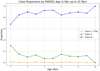 |
Fig. 6 Class proportions by age using uniform 1 Myr bins for sources in the PARSEC age range of 0-10 Myr. The orange line (Class I + Flat) shows consistently low values due to the scarcity of these evolutionary stages in the dataset. Uniform bins were used for consistency and ease of comparison across the age range. The fractions were calculated as the number of sources in each class divided by the total number of sources in the respective age bin. |
5.5 Mass-luminosity relation
The mass-luminosity relation was also analysed using the calculated masses from the PARSEC evolutionary tracks. Fig. 7 shows the masses for 5062 high-confidence sources that fall within the range of the PARSEC evolutionary tracks (solar metallic- ity). A clear upward trend is seen, indicating that as the mass of the stars increases, their luminosity also increases, consistent with the mass-luminosity relation. The relationship appears to be approximately linear for stars with masses between 0.5 and 2 M⊙, consistent with the relation  . For higher masses, likely above 2 Mo , the slope begins to change, suggesting a transition to a region where the exponent becomes approximately 3.5, which corresponds to the main-sequence relation.
As the mass increases, the number of observed stars decreases, particularly for very high masses. This trend is consistent with the understanding that massive stars are less common, and evolve to the main sequence on a shorter timescale.
For low-mass stars, particularly those with masses less than approximately 0.5 M⊙, the relationship between mass and luminosity becomes less straightforward. The study of stellar masses and PMS evolution has seen significant advancements, with several works evaluating the accuracy of different mass determination methods and model predictions (White & Hillenbrand 2004; Bell et al. 2012, 2013). White & Hillenbrand (2004) compared dynamical and evolutionary mass determination techniques using a sample of 115 stars, including both main-sequence and PMS stars. Their results showed generally good agreement for stars with masses above 1.2 M⊙, but for lower-mass stars (down to 0.3 M⊙), evolutionary models consistently underpredicted the masses by 10–30%, with discrepancies as large as 50–100% for stars below 1.0 M⊙. This difference was attributed to inaccuracies in the treatment of convection within the evolutionary models. A similar trend can be observed in Fig. 7, where stars with masses less than 1 Mo show higher luminosities (calculated from SED fitting) and lower masses (derived from stellar evolutionary tracks), highlighting the mass-luminosity mismatch.
Regarding classification, Class I objects are expected to exhibit high luminosities, primarily originating from accretion rather than intrinsic stellar emission. While the Stefan- Boltzmann law provides a reasonable estimate of luminosity based on effective temperature (Teff), the model assumption may not fully capture the complexities of such systems, particularly when circumstellar material is significant. For Class II objects, the observed luminosity is predominantly stellar in origin but remains higher than the ZAMS luminosity, consistent with their pre-main-sequence evolutionary stage. Given the likely contribution from circumstellar material (e.g. a disc), the derived effective temperature (Teff) and radius primarily reflect the stellar component, resulting in an estimate of stellar luminosity rather than the total bolometric luminosity.
The plot effectively illustrates the mass-luminosity relation and provides valuable insights into different stellar classes. The upward trend in luminosity with increasing mass for sources with masses greater than 1 M⊙ is a hallmark of stellar physics and aligns with the empirical relations observed in astrophysics (Kippenhahn & Weigert 1994; Tout et al. 1996; Torres et al. 2010).
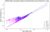 |
Fig. 7 Mass-luminosity plot is presented. This shows mass calculated from PARSEC evolutionary tracks (with solar metallicity) vs luminosity derived from the SED fitting of sources. The colours of the data points represent different classes. |
5.6 FIR/Sub-mm observations and the spatial distribution of YSOs in the OSFC
Previous far-infrared (FIR) studies of the OSFC using Spitzer and other facilities have considerably advanced our understanding of star formation in this region. For instance, Megeath et al. (2012, 2016) and Kounkel et al. (2018) have mapped the distribution of dusty young stellar objects and provided detailed classifications of their evolutionary stages. These works reveal that different regions within the OSFC exhibit distinct characteristics. Specifically, Orion A - particularly around the Orion Nebula Cluster (ONC) - is dominated by very young, embedded protostars (Class I and Flat-spectrum sources), whereas Orion B tends to host a larger fraction of more evolved objects. FIR observations are critical in this context because they detect the dusty envelopes and circumstellar discs that are otherwise challenging to observe, thereby reducing the observational biases that could lead to an underestimation of early-stage star formation.
In the upper panel of Figure 8, we present the spatial distribution of YSOs in the OSFC in RA/Dec coordinates. Gray points denote all detected sources, while yellow points highlight those with at least one valid flux measurement in the FIR/Sub-mm filters (including AllWISE/W4, Spitzer/MIPS, Herschel/PACS, and APEX/LABOCA/SABOCA). Expressing our data in RA/Dec allows for direct comparison with published observational footprints, such as Figure 1 in the Spitzer survey of the Orion A & B molecular clouds Megeath et al. (2012).
The lower panel of Figure 8 shows the spatial distribution of YSO classes derived from our SED fitting across the OSFC. Notably, the regions covered by FIR/Sub-mm observations largely coincide with areas where the youngest objects (Class I and Flat-spectrum sources) are concentrated. This finding is consistent with Spitzer observations and underscores the importance of long-wavelength data for detecting protostellar envelopes and discs. In the absence of such observations, early- stage YSOs may be underestimated, potentially introducing an observational bias. Alternatively, regions lacking Class I and Flat-spectrum sources might be genuinely more evolved, with little circumstellar material remaining. Distinguishing between these possibilities requires a uniform, high-resolution FIR/Sub- mm coverage of the entire complex.
Given that our study incorporates the most comprehensive archival data currently available, our findings are in strong agreement with previous results, reinforcing the established picture of the OSFC’s star-forming regions. While our analysis does not reveal fundamentally new structures, it provides an independent and updated confirmation of the spatial distribution of YSOs and their evolutionary stages, further validating the conclusions drawn from earlier surveys. Our results highlight the importance of continued observational efforts, particularly in the FIR/Sub- mm regime, to refine our understanding of the OSFC’s complex star formation history.
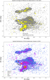 |
Fig. 8 Upper panel shows the observational coverage in the FIR/Sub-mm wavelengths. The lower panel illustrates the spatial distribution of young stellar objects (YSOs) categorized by their evolutionary classes. |
6 Summary
In this study, we have performed a comprehensive SED fitting analysis of YSOs, utilizing a dataset that spans 15 396 sources. The stellar parameters derived from this extensive analysis account for the varying completeness and reliability of the available data. Notably, when considering the more reliable subset of sources that exhibit at least a AllWISE W3 (12 µm) detection at longer wavelengths, with a probability (Prob_W3) greater than 50%, we identify a total of 5062 sources.
The integration of multi-wavelength data is crucial for a more nuanced understanding of star formation. Looking forward, we are incorporating advanced machine learning and deep learning techniques to assist in the identification and classification of YSOs based on their photometric data and light curves. Future work will involve comparing the results obtained through traditional SED fitting methods with those derived from the newly implemented machine learning and deep learning approaches. This comparison will help us assess the strengths and limitations of each method, ultimately refining our understanding of YSOs and their evolutionary processes.
Data availability
The catalog is available at the CDS via anonymous ftp to cdsarc.cds.unistra.fr (130.79.128.5) or via https://cdsarc.cds.unistra.fr/viz-bin/cat/J/A+A/696/A196
Acknowledgements
This work has received funding from the European Union’s Horizon 2020 research and innovation program under grant number 101004141. G.M. acknowledges support from the János Bolyai Research Scholarship of the Hungarian Academy of Sciences. This research was supported by the International Space Science Institute (ISSI) in Bern, through ISSI International Team Project 521 selected in 2021, Revisiting Star Formation in the Era of Big Data (https://teams.issibern.ch/starformation/). IG expresses her thanks to Theo Richardson for his assistance with the updated SED model.
Appendix A Example SED fitting results
Examples of SED fitting results
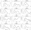 |
Fig. A.1 : SED plots corresponding to the sources listed in Table A.1. These examples illustrate sources at various evolutionary stages, effectively matched with the YSO models from R17. |
References
- Adams, F. C., Lada, C. J., & Shu, F. H. 1987, ApJ, 312, 788 [NASA ADS] [CrossRef] [Google Scholar]
- Allen, L. E., Calvet, N., D’Alessio, P., et al. 2004, ApJS, 154, 363 [Google Scholar]
- Andre, P., & Montmerle, T. 1994, ApJ, 420, 837 [NASA ADS] [CrossRef] [Google Scholar]
- Andre, P., Ward-Thompson, D., & Barsony, M. 1993, ApJ, 406, 122 [NASA ADS] [CrossRef] [Google Scholar]
- Andriantsaralaza, M., Ramstedt, S., Vlemmings, W. H. T., & De Beck, E. 2022, A&A, 667, A74 [NASA ADS] [CrossRef] [EDP Sciences] [Google Scholar]
- Bell, C. P. M., Naylor, T., Mayne, N. J., Jeffries, R. D., & Littlefair, S. P. 2012, MNRAS, 424, 3178 [NASA ADS] [CrossRef] [Google Scholar]
- Bell, C. P. M., Naylor, T., Mayne, N. J., Jeffries, R. D., & Littlefair, S. P. 2013, MNRAS, 434, 806 [NASA ADS] [CrossRef] [Google Scholar]
- Benjamin, R. A., Churchwell, E., Babler, B. L., et al. 2003, PASP, 115, 953 [Google Scholar]
- Bressan, A., Marigo, P., Girardi, L., et al. 2012, MNRAS, 427, 127 [NASA ADS] [CrossRef] [Google Scholar]
- Briceño, C., Calvet, N., Hernández, J., et al. 2019, AJ, 157, 85 [CrossRef] [Google Scholar]
- Chen, Y., Girardi, L., Bressan, A., et al. 2014, MNRAS, 444, 2525 [Google Scholar]
- Chen, Y., Bressan, A., Girardi, L., et al. 2015, MNRAS, 452, 1068 [Google Scholar]
- Cody, A. M., & Hillenbrand, L. A. 2010, ApJS, 191, 389 [NASA ADS] [CrossRef] [Google Scholar]
- Cody, A. M., & Hillenbrand, L. A. 2018, AJ, 156, 71 [Google Scholar]
- Cody, A. M., Stauffer, J., Baglin, A., et al. 2014, AJ, 147, 82 [Google Scholar]
- Crapsi, A., van Dishoeck, E. F., Hogerheijde, M. R., Pontoppidan, K. M., & Dullemond, C. P. 2008, A&A, 486, 245 [NASA ADS] [CrossRef] [EDP Sciences] [Google Scholar]
- Dunham, M. M., Stutz, A. M., Allen, L. E., et al. 2014, in Protostars and Planets VI, eds. H. Beuther, R.S. Klessen, C. P. Dullemond, & T. Henning, 195 [Google Scholar]
- Dunham, M. M., Allen, L. E., Evans, II, N. J., et al. 2015, Astrophys. J. Suppl. Ser., 220, 11 [Google Scholar]
- Eisenhardt, P. R. M., Marocco, F., Fowler, J. W., et al. 2020, ApJS, 247, 69 [Google Scholar]
- Evans, Neal J. I., Dunham, M. M., Jørgensen, J. K., et al. 2009a, ApJS, 181, 321 [Google Scholar]
- Evans, N., Calvet, N., Cieza, L., et al. 2009b, arXiv e-prints [arXiv:0901.1691] [Google Scholar]
- Fazio, G. G., Hora, J. L., Allen, L. E., et al. 2004, ApJS, 154, 10 [Google Scholar]
- Furlan, E., Fischer, W. J., Ali, B., et al. 2016, ApJS, 224, 5 [Google Scholar]
- Gaia Collaboration (Brown, A. G. A., et al.) 2018, A&A, 616, A1 [NASA ADS] [CrossRef] [EDP Sciences] [Google Scholar]
- Gaia Collaboration (Vallenari, A., et al.) 2023, A&A, 674, A1 [NASA ADS] [CrossRef] [EDP Sciences] [Google Scholar]
- Gardner, J. P., Mather, J. C., Clampin, M., et al. 2006, Space Sci. Rev., 123, 485 [Google Scholar]
- Greene, T. P., Wilking, B. A., Andre, P., Young, E. T., & Lada, C. J. 1994, ApJ, 434, 614 [NASA ADS] [CrossRef] [Google Scholar]
- Groβschedl, J. E., Alves, J., Meingast, S., et al. 2018, A&A, 619, A106 [Google Scholar]
- Groβschedl, J. E., Alves, J., Teixeira, P. S., et al. 2019, A&A, 622, A149 [NASA ADS] [CrossRef] [EDP Sciences] [Google Scholar]
- Gutermuth, R. A., Megeath, S. T., Myers, P. C., et al. 2009, ApJS, 184, 18 [Google Scholar]
- Haworth, T. J., Clarke, C. J., Rahman, W., Winter, A. J., & Facchini, S. 2018, MNRAS, 481, 452 [NASA ADS] [CrossRef] [Google Scholar]
- Hernandez, D., Dionatos, O., Audard, M., et al. 2024, A&A submitted [Google Scholar]
- Kippenhahn, R., & Weigert, A. 1994, Stellar Structure and Evolution (Springer Verlag Berlin Heidelberg New York) [Google Scholar]
- Koenig, X. P., & Leisawitz, D. T. 2014, ApJ, 791, 131 [Google Scholar]
- Kounkel, M., Covey, K., Suárez, G., et al. 2018, AJ, 156, 84 [NASA ADS] [CrossRef] [Google Scholar]
- Kuhn, M. A., Hillenbrand, L. A., Sills, A., Feigelson, E. D., & Getman, K. V. 2019, ApJ, 870, 32 [CrossRef] [Google Scholar]
- Lada, C. J. 1987, in Star Forming Regions, 115, eds. M. Peimbert, & J. Jugaku, 1 [NASA ADS] [Google Scholar]
- Lada, C. J. 1987, Symp. Int. Astron. Union, 115, 1 [Google Scholar]
- Lada, C. J., & Wilking, B. A. 1984, ApJ, 287, 610 [NASA ADS] [CrossRef] [Google Scholar]
- Madarász, M., Marton, G., Gezer, I., et al. 2025, A&A, 696, A37 [NASA ADS] [CrossRef] [EDP Sciences] [Google Scholar]
- Mainzer, A., Bauer, J., Cutri, R. M., et al. 2014, ApJ, 792, 30 [Google Scholar]
- Majewski, S. R., Schiavon, R. P., Frinchaboy, P. M., et al. 2017, AJ, 154, 94 [NASA ADS] [CrossRef] [Google Scholar]
- Manara, C. F., Morbidelli, A., & Guillot, T. 2018, A&A, 618, L3 [NASA ADS] [CrossRef] [EDP Sciences] [Google Scholar]
- Manara, C. F., Ansdell, M., Rosotti, G. P., et al. 2023, in Astronomical Society of the Pacific Conference Series, Vol. 534, Protostars and Planets VII, eds. S. Inutsuka, Y. Aikawa, T. Muto, K. Tomida, & M. Tamura, 539 [Google Scholar]
- Marocco, F., Eisenhardt, P. R. M., Fowler, J. W., et al. 2021, ApJS, 253, 8 [Google Scholar]
- Marton, G., Calzoletti, L., Perez Garcia, A. M., et al. 2017, arXiv e-prints [arXiv:1705.05693] [Google Scholar]
- Marton, G., Ábrahám, P., Szegedi-Elek, E., et al. 2019, MNRAS, 487, 2522 [Google Scholar]
- Marton, G., Gezer, I., Madarász, M., et al. 2024, A&A, 688, A203 [NASA ADS] [CrossRef] [EDP Sciences] [Google Scholar]
- Megeath, S. T., Allen, L. E., Gutermuth, R. A., et al. 2004, ApJS, 154, 367 [NASA ADS] [CrossRef] [Google Scholar]
- Megeath, S. T., Flaherty, K. M., Hora, J., et al. 2005, in Massive Star Birth: A Crossroads of Astrophysics, 227, eds. R. Cesaroni, M. Felli, E. Churchwell, & M. Walmsley, 383 [Google Scholar]
- Megeath, S. T., Gutermuth, R., Muzerolle, J., et al. 2012, AJ, 144, 192 [NASA ADS] [CrossRef] [Google Scholar]
- Megeath, S. T., Gutermuth, R., Muzerolle, J., et al. 2016, AJ, 151, 5 [Google Scholar]
- Menten, K. M., Reid, M. J., Forbrich, J., & Brunthaler, A. 2007, A&A, 474, 515 [NASA ADS] [CrossRef] [EDP Sciences] [Google Scholar]
- Morales-Calderón, M., Stauffer, J. R., Hillenbrand, L. A., et al. 2011, ApJ, 733, 50 [CrossRef] [Google Scholar]
- Muzerolle, J., Megeath, S. T., Gutermuth, R. A., et al. 2004, ApJS, 154, 379 [Google Scholar]
- Pilbratt, G. L., Riedinger, J. R., Passvogel, T., et al. 2010, A&A, 518, L1 [NASA ADS] [CrossRef] [EDP Sciences] [Google Scholar]
- Povich, M. S., Smith, N., Majewski, S. R., et al. 2011, VizieR Online Data Catalog, J/ApJS/194/14 [Google Scholar]
- Richardson, T., Ginsburg, A., Indebetouw, R., & Robitaille, T. P. 2024, ApJ, 961, 188 [Google Scholar]
- Rieke, G. H., Young, E. T., Engelbracht, C. W., et al. 2004, ApJS, 154, 25 [Google Scholar]
- Robitaille, T. P. 2017, A&A, 600, A11 [NASA ADS] [CrossRef] [EDP Sciences] [Google Scholar]
- Robitaille, T. P., Whitney, B. A., Indebetouw, R., Wood, K., & Denzmore, P. 2006, ApJS, 167, 256 [Google Scholar]
- Robitaille, T. P., Whitney, B. A., Indebetouw, R., & Wood, K. 2007, Astrophys. J Suppl. S, 169, 328 [Google Scholar]
- Rodrigo, C., & Solano, E. 2020, in XIV.0 Scientific Meeting (virtual) of the Spanish Astronomical Society, 182 [Google Scholar]
- Rodrigo, C., Solano, E., & Bayo, A. 2012, SVO Filter Profile Service Version 1.0, IVOA Working Draft 15 October 2012 [Google Scholar]
- Roquette, J., Audard, M., Hernandez, D., et al. 2025, A&A, submitted [arXiv:2501.08486] [Google Scholar]
- Schlafly, E. F., & Finkbeiner, D. P. 2011, ApJ, 737, 103 [Google Scholar]
- Schlafly, E. F., Meisner, A. M., & Green, G. M. 2019, ApJS, 240, 30 [Google Scholar]
- Silverberg, S. M., Kuchner, M. J., Wisniewski, J. P., et al. 2018, ApJ, 868, 43 [NASA ADS] [CrossRef] [Google Scholar]
- Skrutskie, M. F., Cutri, R. M., Stiening, R., et al. 2006, AJ, 131, 1163 [NASA ADS] [CrossRef] [Google Scholar]
- Stutz, A. M., Tobin, J. J., Stanke, T., et al. 2013, ApJ, 767, 36 [Google Scholar]
- Sutherland, W., Emerson, J., Dalton, G., et al. 2015, A&A, 575, A25 [NASA ADS] [CrossRef] [EDP Sciences] [Google Scholar]
- Tang, J., Bressan, A., Rosenfield, P., et al. 2014, MNRAS, 445, 4287 [NASA ADS] [CrossRef] [Google Scholar]
- Tobin, J. J., Looney, L. W., Li, Z.-Y., et al. 2016, ApJ, 818, 73 [CrossRef] [Google Scholar]
- Tobin, J. J., Sheehan, P. D., Megeath, S. T., et al. 2020, Astrophys. J., 890, 130 [Google Scholar]
- Torres, G., Andersen, J., & Giménez, A. 2010, A&A Rev., 18, 67 [Google Scholar]
- Tout, C. A., Pols, O. R., Eggleton, P. P., & Han, Z. 1996, MNRAS, 281, 257 [Google Scholar]
- Tychoniec, L., Tobin, J. J., Karska, A., et al. 2018, ApJS, 238, 19 [NASA ADS] [CrossRef] [Google Scholar]
- Weingartner, J. C., & Draine, B. T. 2001, ApJ, 548, 296 [Google Scholar]
- Werner, M. W., Roellig, T. L., Low, F. J., et al. 2004, ApJS, 154, 1 [NASA ADS] [CrossRef] [Google Scholar]
- White, R. J., & Hillenbrand, L. A. 2004, ApJ, 616, 998 [Google Scholar]
- Whitney, B. A., Wood, K., Bjorkman, J. E., & Cohen, M. 2003a, ApJ, 598, 1079 [Google Scholar]
- Whitney, B. A., Wood, K., Bjorkman, J. E., & Wolff, M. J. 2003b, ApJ, 591, 1049 [Google Scholar]
- Whitney, B. A., Robitaille, T. P., Bjorkman, J. E., et al. 2013, ApJS, 207, 30 [Google Scholar]
- Wootten, A., & Thompson, A. R. 2009, IEEE Proc., 97, 1463 [NASA ADS] [CrossRef] [Google Scholar]
- Wright, E. L., Eisenhardt, P. R. M., Mainzer, A. K., et al. 2010, AJ, 140, 1868 [Google Scholar]
- Yen, H.-W., & Lee, Y.-N. 2024, ApJ, 972, L27 [NASA ADS] [CrossRef] [Google Scholar]
- Zhang, Y., & Tan, J. C. 2018, ApJ, 853, 18 [Google Scholar]
- Zhao, B., Tomida, K., Hennebelle, P., et al. 2020, Space Sci. Rev., 216, 43 [CrossRef] [Google Scholar]
All Tables
All Figures
|
Fig. 1 Available flux counts for each filter. |
| In the text | |
|
Fig. 2 Luminosity (L) as a function of effective temperature (Teff) is presented. Values are derived from the SED fitting of 15 396 best-fit models and overlaid on the PARSEC evolutionary tracks (with solar metallicity). The data points are colour-coded to represent different stellar classes. |
| In the text | |
|
Fig. 3 Effective temperature (Teff) values from Kounkel et al. (2018) versus the Teff values derived from the SED fitting of 3482 high- confidence sources. Sources, where the best fitting model includes a disc, are plotted with green dots. |
| In the text | |
|
Fig. 4 Colour-colour diagrams for 5062 high-confidence sources, with classes derived from SED fitting. |
| In the text | |
|
Fig. 5 Heatmap showing the distribution of stellar sources across different Stage and Class categories. Stages are derived from SED fitting, while Classes are adopted from Hernandez et al. (2024), providing a visual representation of the relationship between stellar evolutionary stages and classifications. |
| In the text | |
|
Fig. 6 Class proportions by age using uniform 1 Myr bins for sources in the PARSEC age range of 0-10 Myr. The orange line (Class I + Flat) shows consistently low values due to the scarcity of these evolutionary stages in the dataset. Uniform bins were used for consistency and ease of comparison across the age range. The fractions were calculated as the number of sources in each class divided by the total number of sources in the respective age bin. |
| In the text | |
|
Fig. 7 Mass-luminosity plot is presented. This shows mass calculated from PARSEC evolutionary tracks (with solar metallicity) vs luminosity derived from the SED fitting of sources. The colours of the data points represent different classes. |
| In the text | |
|
Fig. 8 Upper panel shows the observational coverage in the FIR/Sub-mm wavelengths. The lower panel illustrates the spatial distribution of young stellar objects (YSOs) categorized by their evolutionary classes. |
| In the text | |
|
Fig. A.1 : SED plots corresponding to the sources listed in Table A.1. These examples illustrate sources at various evolutionary stages, effectively matched with the YSO models from R17. |
| In the text | |
Current usage metrics show cumulative count of Article Views (full-text article views including HTML views, PDF and ePub downloads, according to the available data) and Abstracts Views on Vision4Press platform.
Data correspond to usage on the plateform after 2015. The current usage metrics is available 48-96 hours after online publication and is updated daily on week days.
Initial download of the metrics may take a while.