| Issue |
A&A
Volume 696, April 2025
|
|
|---|---|---|
| Article Number | A231 | |
| Number of page(s) | 6 | |
| Section | The Sun and the Heliosphere | |
| DOI | https://doi.org/10.1051/0004-6361/202452524 | |
| Published online | 25 April 2025 | |
Understanding coronal rain dynamics through a point-mass model
1
Department of Mathematics and Statistics, University of Exeter, Exeter EX4 4QF, UK
2
Departament de Física, Universitat de les Illes Balears, E-07122 Palma de Mallorca, Spain
3
Institut d’Aplicacions Computacionals de Codi Comunitari (IAC3), Universitat de les Illes Balears, E-07122 Palma de Mallorca, Spain
4
Instituto de Astrofísica de Canarias, E-38205 La Laguna, Tenerife, Spain
5
Departamento de Astrofísica, Universidad de La Laguna, E-38205 La Laguna, Tenerife, Spain
⋆ Corresponding author: a.s.hillier@exeter.ac.uk
Received:
7
October
2024
Accepted:
5
March
2025
Aims. Observations and simulations of coronal rain show that as cold and dense plasma falls through the corona, it initially undergoes acceleration by gravity before the downward velocity saturates. Simulations have shown the emergence of an unexpected relation between the terminal velocity of the rain and density ratio that has not been explained. Our aim is to explain this relation.
Methods. We developed a simple point-mass model to understand how the evolution of the ambient corona moving with the coronal rain drop can influence the falling motion.
Results. We find that this simple effect results in the downward speed reaching a maximum value before decreasing, which is consistent with simulations with realistic coronal rain mass. These results provide an explanation for the scaling of the maximum downward speed to density ratio of the rain to the corona, and as such, they provide a new tool that may be used to interpret observations.
Key words: hydrodynamics / magnetic fields / magnetohydrodynamics (MHD)
© The Authors 2025
 Open Access article, published by EDP Sciences, under the terms of the Creative Commons Attribution License (https://creativecommons.org/licenses/by/4.0), which permits unrestricted use, distribution, and reproduction in any medium, provided the original work is properly cited.
This article is published in open access under the Subscribe to Open model. Subscribe to A&A to support open access publication.
1. Introduction
Quiescent coronal rain is a multiphase plasma phenomenon of cool plasma embedded in a hot component that is frequently observed in solar active regions (Antolin 2020; Antolin & Froment 2022; Şahin & Antolin 2022; Şahin et al. 2023). It starts with the continuous evaporation of cold and dense plasma from the solar chromosphere into the corona. This evaporated plasma, which now has the typical hot and rarefied conditions of the corona, accumulates at the apex of a coronal loop and eventually becomes thermally unstable (Parker 1953; Field 1965; Antiochos 1980), which leads to the formation of a dense coronal rain clump some tens of megametres high in the corona. Electron number densities of the order of 2 − 25 × 1010 cm−3 have been measured by Antolin et al. (2015), compared to characteristic coronal loop densities in active regions of the order of 1 − 10 × 109 cm−3 (Reale 2010). These values translate into clump densities of the order of 3 − 40 × 10−14 g cm−3 (note that post-flare coronal rain can reach higher densities; see Şahin & Antolin 2024, who report values ∼10−12 g cm−3). After this formation phase, coronal rain falls along the loop legs toward the solar surface under the action of gravity, although in many cases it does not attain the gravitational free-fall speed, but instead reaches a constant (or even decreasing) velocity. Coronal rain typically reaches falling speeds of up to 150 km s−1 (see, for example, Wiik et al. 1996; Antolin & Rouppe van der Voort 2012; Kriginsky et al. 2021).
The descending phase of coronal rain is characterised by the cold and dense plasma flowing along coronal loops that are aligned with the coronal magnetic field (see, e.g., Tripathi et al. 2006, 2007), implying that some inherent aspects of the dynamics are essentially one-dimensional (1D). This was used by Oliver et al. (2014) to set up 1D hydrodynamic models of coronal rain that reproduced the observed smaller-than-free-fall speed. These authors also found that coronal rain blobs achieve a maximum descending velocity, after which their speed is reduced gradually in time. The work of Oliver et al. (2014) was extended to 2D by Martínez-Gómez et al. (2020). A very interesting aspect of the simulations of Martínez-Gómez et al. (2020) is that in the limit of a strong magnetic field, that is, |B|≳20 G, the simulated coronal rain dynamics effectively became the sum of a set of vertical 1D models of the type presented in Oliver et al. (2014), meaning that 1D modelling is reasonable given the strong magnetic field of the solar corona as this implies that the Alfvén Mach number and plasma beta of the coronal rain are small (magnetic field strengths of the order of hundreds of Gauss or even larger have been inferred by Schad et al. 2016; Kuridze et al. 2019; Kriginsky et al. 2021). Both in Martínez-Gómez et al. (2020) and in other multi-dimensional simulations using weaker field strengths (e.g. Fang et al. 2015), it has been found that there is a greater influence of multi-dimensional effects. Assessing the dynamics of their simulated rain blobs, Martínez-Gómez et al. (2020) found through an empirical fit that the maximum downward velocity of the falling coronal rain scales as the rain-to-corona density ratio to the power 0.64 (i.e. (ρrain/ρcorona)0.64). A key question that still remains is what causes this particular exponent.
One possible way of understanding the dynamics of these simulations may be through simplified point-mass and drag models. These models have been widely applied in many areas of fluid dynamics, including the modelling of coronal mass ejection (CME) propagation (e.g. Vršnak et al. 2010, 2013). A standard aspect of drag models is that the faster the body moves, the stronger the drag force works to decelerate it. Physically, this relates to the moving structure having to do more work to push aside the ambient material as it moves faster. This model predicts a terminal fall velocity that scales (in the high-density-ratio limit) as approximately the density ratio to the power 0.5 (e.g. Zhou et al. 2021). This discrepancy to the exponent found by Martínez-Gómez et al. (2020) for their simulations is interesting as it implies that some different physics needs to be considered.
Another key aspect of point-mass models, including drag models, is that as the mass moves through the medium, a portion of the ambient fluid, which we refer to as the virtual mass, moves with the body. In effect, this adds to the mass of the moving body. For a standard drag problem, including one that involves incompressible flow, the virtual mass of the system is expected to not change significantly over time (e.g. as used in Vršnak et al. 2010, 2013). If the mass of the body is higher than that of the virtual mass, then the virtual mass does not change the dynamics in any significant way. Due to the high mass of a coronal rain blob, we may naturally expect this to be the case. However, this assumption may not hold for the coronal rain falling along magnetic field as a significant amount of material in front of and behind the moving coronal rain has to move as well.
We develop a simple model for the coronal rain dynamics simulated by Oliver et al. (2014) and Martínez-Gómez et al. (2020) by considering the role of virtual mass to quantify how it controls the evolution of the rain motion. We then use this model to provide an explanation for the density and coronal rain velocity scaling presented in Martínez-Gómez et al. (2020).
2. An overview of the numerical modelling
We considered a 1D vertical slice of a fully ionised hydrogen plasma. The adiabatic hydrodynamic evolution of this system is described by the continuity equations of mass, momentum, and pressure,
Here, t and z are time and the vertical coordinate, with the z-axis pointing upward; ρ(z, t), v(z, t) and p(z, t) are the density, vertical velocity component, and pressure; g = 274 m s−2 is the acceleration of gravity at the solar surface; and γ = 5/3 is the ratio of specific heats.
In an isothermal atmosphere with temperature T0, the plasma is in hydrostatic equilibrium, with pressure and density given by
where the vertical scale height H is

with kB the Boltzmann constant and mp the proton mass. To derive Equation (6), we used the perfect gas law for a fully ionised hydrogen gas,
Now, we study the temporal evolution of the system with zero initial velocity, initial pressure given by Equation (4), and initial density given by the sum of Equation (5) plus a blob density,
![$$ \begin{aligned} \rho _{\rm b}(z) = \rho _{\rm b0} \exp \left[-\left(\frac{z-z_0}{\Delta }\right)^2\right]. \end{aligned} $$](/articles/aa/full_html/2025/04/aa52524-24/aa52524-24-eq8.gif)
To obtain ρ(z, t), v(z, t), and p(z, t), we performed numerical simulations as described in Oliver et al. (2014). The problem parameters were the background homogeneous temperature, T0, the density at the z = 0 height, ρ0, the initial height of the dense blob, z0, and the blob density and length, ρb0 and Δ. The pressure at the z = 0 height, p0, appears in Equation (4) and can be determined from T0 and ρ0 with the help of Equation (7). With no loss of generality, we set ρ0 = 5 × 10⁻¹² kg m−3 and z0 = 50 Mm. Hence, we were left with three free parameters, namely T0 (or H), ρb0, and Δ.
The temporal evolution of the system is as follows: The introduction of a density enhancement at z = z0 sends two sound waves travelling up and down at the (constant) sound speed  . The blob also starts to fall with a subsonic speed (see Figure 1a and the corresponding movie) until it reaches a maximum downward velocity, vb, max, after which it presents a gentle deceleration. This behaviour of the blob velocity is shown in Figures 2a–c. Oliver et al. (2014) found an unexpected association between vb, max and the ratio of the blob density to the local ambient density at t = 0; here we denote this density ratio as dr. This association is surprising because atmospheres with different T0 have different scale heights, and although the blob falls through atmospheres with a different stratification, it appears that only the initial ambient density at height z0 matters. The plot of vb, max versus dr in Oliver et al. (2014) was presented for Δ = 0.5 Mm. Changes to this parameter lead to increases or decreases of the blob mass, and therefore, to larger or smaller vb, max, respectively, and the already mentioned association is not fulfilled. To correct for this fact, we can plot vb, max as a function of Δdr, as shown in Figure 2d, which results in the points aligning relatively neatly along a curve with little, but non-negligible, spread.
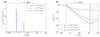 |
Fig. 1. Results of three numerical simulations with with T0 = 2 × 10⁶ K, Δ = 0.5 Mm, and ρb0 = 10−10 kg m−3 (red), ρb0 = 5 × 10⁻¹⁰ kg m−3 (green), and ρb0 = 10 × 10−10 kg m−3 (blue). (a) Density as a function of height at a given time. (b) Velocity as a function of height at a given time. A dashed vertical black line is plotted at z = z0 − Cst giving the position of the front of the compression wave. The dashed vertical red, green, and blue lines give the position of the maximum density. Animations of these figures can be found online. |
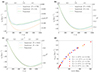 |
Fig. 2. Blob velocity as a function of time for three setups with T0 = 2 × 10⁶ K, Δ = 0.5 Mm, and (a) ρb0 = 10−10 kg m−3, (b) ρb0 = 5 × 10⁻¹⁰ kg m−3, and (c) ρb0 = 10 × 10−10 kg m−3. The green curve comes from the numerical solution of Equations (1)–(3), whereas the analytical approximation of Equation (18) is given by the blue and orange curves for the best fit of D and for D = 0.6, respectively. The variables τ and Vb are the dimensionless time and blob speed (see Section 3.2). (d) (Unsigned) maximum blob velocity, vb, max, vs. Δ dr (the meaning of the different symbols is given in the figure legend). |
In addition, the falling blob pushes down the gas below it and also pulls down the gas above it. In other words, part of the vertical mass column is set into motion because of the presence of the density enhancement. The lower and upper points of this mass column travel at speed Cs, and hence, at time t, they have coordinates z = z0 ± Cst (see Figure 1b and the corresponding movie). The two boundaries of the numerical domain are placed at a large distance from the initial blob position, and this prevents the sound waves that bounce off the boundaries from interfering with the blob dynamics (for more details, see Oliver et al. 2014).
3. The importance of virtual mass
Our aim in this paper is to develop a simple analytic model for the motion of coronal rain as presented in the simulations of Oliver et al. (2014) and Martínez-Gómez et al. (2020). Having seen from the simulations presented in Section 2 that a large region of the corona responds to the motion of the coronal rain (see Figure 1b), the implication of this is that the ambient mass (i.e. the virtual mass) is evolving and can be significant. Therefore, the key question we need to determine first is the virtual mass for our problem. There are two key pieces of information from the works of Oliver et al. (2014), Martínez-Gómez et al. (2020) and Section 2 that we used: (1) For a strong magnetic field, the 2D dynamics becomes 1D like, therefore we only look to model 1D dynamics using a point mass, and (2) two waves, a compression wave propagating downward and a rarefaction wave propagating upward, are set off as the blob starts to move. The fronts of these waves propagate at the sound speed of the ambient medium. The distance these wave fronts have propagated at a given time determines the amount of the ambient mass (i.e. the virtual mass) that can respond to the motion. The growth of the virtual mass in time is shown in Figure 1b and the accompanying movie, in which the vertical black line separates the unperturbed and perturbed plasma below and above this height, respectively. As time evolves, the height represented by the vertical line moves down at the constant speed Cs. This means that unlike a standard drag model, the virtual mass evolves over time.
This leads to the question how we can include this dynamically evolving virtual mass into a simple drag-like model. When we treat our coronal rain blob as a mass (mb) falling through a vacuum, then we get this simple equation for the dynamics
The virtual mass (mv) takes momentum from the coronal rain and places it into the surrounding material. Treating the virtual mass as being able to respond instantly to changes in the momentum of the blob, we need to add two terms to Equation (9): One term to show how change in the speed of the blob increases the speed of the virtual mass, and another term to represent the change in the virtual mass, because it is a growing region due to the continued propagation of the sound waves, increasing the momentum of the virtual mass (and reducing the momentum of the blob). This leads to
where vv is the velocity of the virtual mass.
We do not know vv (as with vb, it will not be a single value, but we treat it as such; this can be seen by the broad velocity distributions in Figure 1b going from zero at the compression wave front to a maximum at the blob position), and as it relates to how the mass in front of and behind the blob moves, it will be some factor (which may not be constant) of the blob velocity which we denote D(t). This means we represent the average speed of the material in front of and behind the moving blob as D(t)vb. This gives
or
where we assumed that the coronal rain mass (mb) is constant. Equation (12) does not include any drag term, and it can be used to obtain a formula for the velocity at a given time. This latter formula is
We now consider some specific situations for understanding the evolution of the virtual mass and how this influences the dynamics. We note here that we take D(t) to be a constant D for the rest of this section. We are then able to confirm the validity of this assumption when comparing to simulation results.
3.1. Virtual mass in a constant-density background
Before we consider a stratified atmosphere, it is informative to investigate the case of a constant-density background (ρ0) with a constant sound speed (Cs). We have the mass of the blob given by mb = SFbρ0hb, where ρ0 is the density of the corona where the blob is placed, Fb is the increase factor of the density, S is the cross-sectional area, and hb is a measure of the blob length (to take this from density to mass). The conversion between Δ (the half-width of the Gaussian distribution) in Oliver et al. (2014) and this model is  as this means that the value of Fb used here directly relates to the density ratio of Oliver et al. (2014) and the simulations of Section 2. For the virtual mass, we know that the mass in causal contact with the moving blob can be given by
Based on these arguments, we have
We can quickly see that at early times, the downward velocity will increase at an approximately linear rate that is consistent with free-fall. However, at late times, the denominator will approximately scale linearly with time, leading to the downward velocity converging to a value of
This simple model shows that we expect the final velocity to be linearly proportional to the density ratio. However, this does not have the earlier peak in velocity with a slow decline afterwards that is seen in Figure 2.
3.2. Virtual mass in a stratified atmosphere
Our next step was to develop the model to include a stratified atmosphere with constant sound speed to mimic the simulations presented in Section 2. This led to a more complex evolution of the virtual mass. Setting the position where the blob is placed to be z = 0, we then have
![$$ \begin{aligned} m_{\rm v}&= \rho _0S\int _{-C_{\rm s}t}^{C_{\rm s}t}\exp (-z/H) \mathrm{d}z \\&=H\rho _0S\left[\exp \left(\frac{C_{\rm s} t}{H}\right)- \exp \left(-\frac{C_{\rm s} t}{H}\right)\right]=2H\rho _0S\sinh \left(\frac{C_{\rm s} t}{H}\right),\nonumber \end{aligned} $$](/articles/aa/full_html/2025/04/aa52524-24/aa52524-24-eq19.gif)
with H as the pressure scale height. Justification for this range of integration is shown in Figure 1b, which shows that for any initial coronal rain mass, the region of the ambient corona that is influenced by its motion is restricted to the regions in causal contact as determined by the propagation of the front of the compression and rarefaction waves that travel at the ambient sound speed. With this new formula for the virtual mass, this gives us
As t/sinh(Cst/H) tends to zero as t tends to infinity, this implies that vb will tend to zero at large times. However, for small (but non-zero) t, we have a situation that is equivalent to the constant-density case, so that the downward velocity will initially increase in magnitude with vb ∝ t.
The results from this model are overplotted as the dashed orange and blue lines in Figures 2a–c. The dashed blue line is the solution for a value of D that was optimised to give the best fit to vb(t), and the orange line is for a value of D = 0.6. Both these curves give acceleration of the coronal rain downwards and then deceleration as the virtual mass becomes significant. Figures 2a–c show that as the mass of the coronal rain is increased, the simulation results become closer to those of the D = 0.6 curve. The value of D = 0.6 implies that the average velocity of the virtual mass is more weighted to the blob mass than would be found for a linear velocity profile. The velocity profiles in Figure 1b show that such a profile is found in the simulations.
To make further progress (i.e. to remove the temperature effects from the equation), we can non-dimensionalise Equation (18). Firstly, we set τ = Cst/H. This gives (taking D to be constant)
From this equation, we see we have the free-fall velocity after a sound crossing time (gH/Cs) and the ratio of the blob mass to the mass in a pressure scale height (M = Fbhb/H) as fundamental quantities of the system. This leads to the non-dimensionalised equation
with Vb = vbCs/(gH).
The next step was to determine the relation between M and the maximum value of Vb (Vb, max). By taking the derivative of Equation (20) with respect to τ, we find

with τmax the value of τ associated with Vb, max. Using this to remove M from Equation (20) gives

Although this does not give a direct analytic formula for the dependence of Vb, max on M, it does allow them to be directly connected.
The simulation results are plotted using this new normalisation in Figure 3. This shows the various different models collapsed onto the same curve, and it confirms that the non-dimensionalisation correctly captures the underlying physics of the problem. The dashed line is the analytic prediction stated above using D = 0.6. At small M, the model slightly over-predicts the value of Vb, max. However, above M ≈ 1, the simulation results and the model align to a good degree. It should also be noted that using the normalisation in this figure, the small spread that can be seen in the simulation results presented in Figure 2d is completely removed.
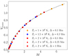 |
Fig. 3. Plot of (unsigned) maximum Vb against M for the simulation results (the meaning of the different symbols is given in the figure legend). The dashed line is the predicted value from Equation (20) with D = 0.6. |
4. Summary and discussion
We have presented a simple model for the dynamics of coronal rain that provides an explanation of much of the behaviour found in the simulations of rain evolution by Oliver et al. (2014). The key process is that the corona responds over a large distance (determined by the propagation of sound waves) to the motion of the coronal rain to effectively add mass to the system, which in turn reduces its speed. A particular key result is that the scaling of the maximum downflow speed as a function of the density ratio to the power 0.64 given by a fit to the data in Martínez-Gómez et al. (2020) here is explained by an analytic relation that appears to have a similar trend to this power law.
As we were able to show that the model for virtual mass effectively decelerating the coronal rain in the model of Oliver et al. (2014), this leads to the question of which role, if any, a drag-like (by this we mean a term ∝vb2) force plays. Figure 3 shows that for low M values, the value of Vb, max from the simulations is lower than we predicted from our model. For these low-mass cases, it is likely that pressure gradients acting to give an upward force are created by the downward motion of the coronal rain, and these can act as a drag. However, for a higher rain mass (i.e. M ⪆ 1.5, which is more consistent with the mass of the solar atmosphere), this effect becomes small.
Finally, an important question to ask is whether we can reasonably assume that D(t) will be constant in time and will have the same value for the regions above and below the coronal rain. Figure 2 shows that for a high rain mass, the model provides a good representation of the velocity evolution over a long time (i.e. M ⪆ 1.5, the lower bound of which corresponds to Figure 2b), meaning that changes in the value should be small. However, at very high (i.e. M ⪆ 6) rain masses, the downflow velocity may become trans- or super-sonic, which will change the way in which the rain motion is transmitted into the surrounding corona. This will likely result in the value of D evolving over time. Relevant to this, some observations have implied that strong compression (Antolin et al. 2023) or shocks (Schad et al. 2016) precede coronal rain blobs. Compression in front of the rain as it moves is a fundamental aspect of our model. Therefore, observations may create a pathway to calculate the value of D for real dynamics. In addition to this, shock formation is something that our model implies as a possibility, and an important further step will be calculating the relevant M values for the observations to determine whether we predict a transonic flow.
As a final comment, simplified drag models are widely used in understanding and modelling dynamics in a broad range of situations, including CME propagation (e.g. Vršnak et al. 2010) and the dynamics of cool, dense clouds of gas in fast outflows found in the intracluster medium (e.g. Gronke & Oh 2018). However, our model with evolving virtual mass is more relevant for situations with a strong magnetic field, as quantified by having sub-Alfvénic flow speeds in a low-β plasma environment. This is a fundamental difference from the examples listed above, where weaker magnetic fields mean that aerodynamic drag is the dominant process influencing the temporal evolution. The ideas that underpin our model are therefore likely to be applicable in situations in which motion is confined to flow along the magnetic field; an example of this may be accretion to the poles of highly magnetised neutron stars (e.g. Davidson 1973), presenting some further avenues for this work.
Data availability
Movies associated to Fig. 1 are available at https://www.aanda.org
Acknowledgments
AH is supported by STFC Research Grant No. ST/R000891/1 and ST/V000659/1. DM acknowledges support from the Spanish Ministry of Science and Innovation through the grant CEX2019-000920-S of the Severo Ochoa Program. This publication is part of the R+D+i project PID2023-147708NB-I00, financed by MICIU/AEI/10.13039/501100011033/ and FEDER, EU. AH and RO would like to acknowledge the discussions with members of ISSI Team 457 “The Role of Partial Ionization in the Formation, Dynamics and Stability of Solar Prominences” and ISSI Team 545 “Observe Local Think Global: What Solar Observations can teach us about Multiphase Plasmas across Astrophysical Scales”, which have helped improve the ideas in this manuscript. We would also like to thank the anonymous referee for their useful comments. The simulation data presented in Section 2 is based on the work of Oliver et al. (2014) and will be made available on reasonable request. There are no other data produced for this paper.
References
- Antiochos, S. K. 1980, ApJ, 241, 385 [NASA ADS] [CrossRef] [Google Scholar]
- Antolin, P. 2020, Plasma Phys. Control. Fusion, 62, 014016 [Google Scholar]
- Antolin, P., & Froment, C. 2022, Front. Astron. Space Sci., 9, 820116 [NASA ADS] [CrossRef] [Google Scholar]
- Antolin, P., & Rouppe van der Voort, L. 2012, ApJ, 745, 152 [Google Scholar]
- Antolin, P., Vissers, G., Pereira, T. M. D., Rouppe van der Voort, L., & Scullion, E. 2015, ApJ, 806, 81 [Google Scholar]
- Antolin, P., Dolliou, A., Auchère, F., et al. 2023, A&A, 676, A112 [NASA ADS] [CrossRef] [EDP Sciences] [Google Scholar]
- Davidson, K. 1973, Nat. Phys. Sci., 246, 1 [NASA ADS] [CrossRef] [Google Scholar]
- Fang, X., Xia, C., Keppens, R., & Doorsselaere, T. V. 2015, ApJ, 807, 142 [NASA ADS] [CrossRef] [Google Scholar]
- Field, G. B. 1965, ApJ, 142, 531 [Google Scholar]
- Gronke, M., & Oh, S. P. 2018, MNRAS, 480, L111 [Google Scholar]
- Kriginsky, M., Oliver, R., Antolin, P., Kuridze, D., & Freij, N. 2021, A&A, 650, A71 [NASA ADS] [CrossRef] [EDP Sciences] [Google Scholar]
- Kuridze, D., Mathioudakis, M., Morgan, H., et al. 2019, ApJ, 874, 126 [Google Scholar]
- MartÃnez-Gómez, D., Oliver, R., Khomenko, E., & Collados, M. 2020, A&A, 634, A36 [Google Scholar]
- Oliver, R., Soler, R., Terradas, J., Zaqarashvili, T. V., & Khodachenko, M. L. 2014, ApJ, 784, 21 [Google Scholar]
- Parker, E. N. 1953, ApJ, 117, 431 [Google Scholar]
- Reale, F. 2010, Liv. Rev. Sol. Phys., 7, 5 [Google Scholar]
- Åžahin, S., & Antolin, P. 2022, ApJ, 931, L27 [CrossRef] [Google Scholar]
- Åžahin, S., & Antolin, P. 2024, ApJ, 970, 106 [Google Scholar]
- Åžahin, S., Antolin, P., Froment, C., & Schad, T. A. 2023, ApJ, 950, 171 [CrossRef] [Google Scholar]
- Schad, T. A., Penn, M. J., Lin, H., & Judge, P. G. 2016, ApJ, 833, 5 [Google Scholar]
- Tripathi, D., Solanki, S. K., Schwenn, R., et al. 2006, A&A, 449, 369 [NASA ADS] [CrossRef] [EDP Sciences] [Google Scholar]
- Tripathi, D., Solanki, S. K., Mason, H. E., & Webb, D. F. 2007, A&A, 472, 633 [NASA ADS] [CrossRef] [EDP Sciences] [Google Scholar]
- Vršnak, B., Žic, T., Falkenberg, T. V., et al. 2010, A&A, 512, A43 [CrossRef] [EDP Sciences] [Google Scholar]
- Vršnak, B., Žic, T., Vrbanec, D., et al. 2013, Sol. Phys., 285, 295 [CrossRef] [Google Scholar]
- Wiik, J. E., Schmieder, B., Heinzel, P., & Roudier, T. 1996, Sol. Phys., 166, 89 [NASA ADS] [CrossRef] [Google Scholar]
- Zhou, Y., Williams, R. J. R., Ramaprabhu, P., et al. 2021, Phys. D Nonlinear Phenom., 423, 132838 [NASA ADS] [CrossRef] [Google Scholar]
All Figures
|
Fig. 1. Results of three numerical simulations with with T0 = 2 × 10⁶ K, Δ = 0.5 Mm, and ρb0 = 10−10 kg m−3 (red), ρb0 = 5 × 10⁻¹⁰ kg m−3 (green), and ρb0 = 10 × 10−10 kg m−3 (blue). (a) Density as a function of height at a given time. (b) Velocity as a function of height at a given time. A dashed vertical black line is plotted at z = z0 − Cst giving the position of the front of the compression wave. The dashed vertical red, green, and blue lines give the position of the maximum density. Animations of these figures can be found online. |
| In the text | |
|
Fig. 2. Blob velocity as a function of time for three setups with T0 = 2 × 10⁶ K, Δ = 0.5 Mm, and (a) ρb0 = 10−10 kg m−3, (b) ρb0 = 5 × 10⁻¹⁰ kg m−3, and (c) ρb0 = 10 × 10−10 kg m−3. The green curve comes from the numerical solution of Equations (1)–(3), whereas the analytical approximation of Equation (18) is given by the blue and orange curves for the best fit of D and for D = 0.6, respectively. The variables τ and Vb are the dimensionless time and blob speed (see Section 3.2). (d) (Unsigned) maximum blob velocity, vb, max, vs. Δ dr (the meaning of the different symbols is given in the figure legend). |
| In the text | |
|
Fig. 3. Plot of (unsigned) maximum Vb against M for the simulation results (the meaning of the different symbols is given in the figure legend). The dashed line is the predicted value from Equation (20) with D = 0.6. |
| In the text | |
Current usage metrics show cumulative count of Article Views (full-text article views including HTML views, PDF and ePub downloads, according to the available data) and Abstracts Views on Vision4Press platform.
Data correspond to usage on the plateform after 2015. The current usage metrics is available 48-96 hours after online publication and is updated daily on week days.
Initial download of the metrics may take a while.