| Issue |
A&A
Volume 696, April 2025
|
|
|---|---|---|
| Article Number | A209 | |
| Number of page(s) | 5 | |
| Section | The Sun and the Heliosphere | |
| DOI | https://doi.org/10.1051/0004-6361/202451526 | |
| Published online | 23 April 2025 | |
Ionization memory of plasma emitters in a solar prominence
1
Institut für Astrophysik, Universität Göttingen, Friedrich-Hund-Platz 1, 37077 Göttingen, Germany
2
Leibniz-Institut für Astrophysik Potsdam (AIP), An der Sternwarte 16, 14482 Potsdam, Germany
3
Institute d’Astrophysique, 98 bis Boulevard Arago, 75014 Paris, France
4
Istituto ricerche solari Aldo e Cele Daccó (IRSOL), Universitá della Svizzera italiana, Via Patocchi 57, 6605 Locarno-Monti, Switzerland
⋆ Corresponding author: This email address is being protected from spambots. You need JavaScript enabled to view it.
Received:
16
July
2024
Accepted:
7
March
2025
Abstract
Aims. In the low-collisional, partially ionized plasma (PIP) of solar prominences, uncharged emitters might show different signatures of magnetic line broadening than charged emitters. We investigate if the widths of weak metal emissions in prominences exceed the thermal line broadening by a different amount for charged and for uncharged emitters.
Methods. We simultaneously observe five optically thin, weak metal lines in the brightness center of a quiescent prominence and compare their observed widths with the thermal broadening.
Results. The inferred nonthermal broadening of the metal lines does not indicate systematic differences between the uncharged Mg b2 and Na D1 and the charged Fe II emitters, only Sr II is broader.
Conclusions. The additional line broadening of charged emitters can reasonably be attributed to magnetic forces. That of uncharged emitters can then come from their temporary state as ions before recombination. Magnetically induced velocities will be retained some time after recombination. Modelling PIPs then requires consideration of a memory of previous ionization states.
Key words: methods: observational / techniques: spectroscopic / Sun: filaments, prominences
Deceased on 03 February 2025.
© The Authors
 Open Access article, published by EDP Sciences, under the terms of the Creative Commons Attribution License (https://creativecommons.org/licenses/by/4.0), which permits unrestricted use, distribution, and reproduction in any medium, provided the original work is properly cited.
This article is published in open access under the Subscribe to Open model. This email address is being protected from spambots. You need JavaScript enabled to view it. to support open access publication.
1. Introduction
The study of partially ionized plasmas (PIPs) has become increasingly important in recent years (Khomenko 2017; Ballester et al. 2018; Soler & Ballester 2022; Parenti et al. 2024; Heinzel et al. 2024). A reduced collisional rate of a PIP enables a decoupling of charged and uncharged species, which leads to their different dynamical behavior. Higher flow velocities (line shifts) of ions are observed by Khomenko et al. (2016), Wiehr et al. (2019, 2021), and Zapiór et al. (2022) in solar prominences, which are ideal objects for observing such effects with high spatial and temporal resolution. Drifts of ions relative to neutrals pose a particular problem for prominence support against gravity by magnetic forces, since neutrals will sink through the magnetic structure if they are not in collisional equilibrium with charged particles. Gilbert et al. (2002, 2007) report a depletion of helium in the high parts of filaments. For prominences, we expect a certain coupling between the two, but weak enough to allow drifts between ions and neutrals.
The decoupling of charged and uncharged species in a PIP can also manifest itself in a different line broadening. Landman (1981) already expected lines from ions to be broader than those from neutrals. Ramelli et al. (2012) found, for a quiescent prominence, a He II line 1.5 times broader than a He I line from the triplet system which, in turn, is 1.1 times broader than a He I line from the singlet system. Stellmacher & Wiehr (2015) find that the Mg b2 line is 1.3 times broader than the (“forbidden”) inter-combination line from the magnesium triplet to the singlet system. Stellmacher & Wiehr (2017) find a width excess of Sr II and Fe II lines relative to Na D and the He-singlet, respectively, which they interpret as being due to influences of magnetic forces. González Manrique et al. (2024) observe the Ca II 8542 Å line as broader than expected from He D3 and Hα. Since strong (chromospheric) lines such as Ca II 8542 Å and Hα are optically thick in most parts of a prominence, the result is limited to the boundary between the prominence and the corona where “instabilities may take place… helping to increase the differential ion-neutral behavior…” (González Manrique et al. 2024). Pontin et al. (2020) investigate for coronal loops such line broadening in terms of magnetic “braiding induced turbulence”, but it is not fully clear if such an effect also applies in prominences.
Parenti et al. (2024) resume that “we need the measurement of several spectral profiles from neutrals and low ionization state species under optical thin condition”. This is the aim of the present study. We observe weak metal lines which are optically thin throughout the whole prominence allowing us to analyze the line broadening in the central prominence body. Such weak metal lines are rarely observed in prominences; they are mostly drowned in the parasitic light of the aureole and therefore require careful correction as opposed to what is needed for bright chromospheric lines.
2. Observations and data reduction
We improved previous sequential measurements by simultaneous observations of seven emission lines in a prominence using the Télescope Héliospherique pour l’Etude de Magnétisme et des Instabilités Solaires (THEMIS) on Tenerife and its echelle spectrograph. The prominence at the west limb, 52°N, on June 6, 2022 shows negligible evolutionary variation (according to images from the Global Oscillation Network Group, GONG, data archive) and can thus be considered as quiescent. Since slit-jaw images were not available, we reconstructed the slit positions in a prominence image from the GONG survey using the observed distribution of the Hγ intensity along each slit position (Fig. 1).
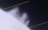 |
Fig. 1. Hα image of the prominence at the west limb, 52° north, from June 6, 2022, (GONG archive); North direction is upward; the long lines mark the direction of refraction at two slit positions beside the prominence used for the determination of parasitic light; the short lines mark slit positions reconstructed from the observed Hγ intensity variation and their extension of 12″ corresponds to 8.7 Mm. |
Given the different wavelengths of the observed lines, the spectrograph slit is reasonably aligned along the direction of refraction which varies throughout the day. Therefore, a spectrograph slit constantly oriented along the direction of refraction will rotate over the prominence. Near solstice, however, its direction remains almost constant for a few hours (see Wiehr et al. 2019). We observed from 9:06 to 9:24 UT and accordingly kept the slit at an angle of 72° clockwise from north, its width corresponding to  (≈1000 km on the Sun). Five cameras recorded the emission lines Hγ, Na D1, and Sr II 4216 Å, and the neighboring line pairs He I 5015 Å and Fe II 5018 Å, and Fe II 5169 Å and Mg b2 5172 Å. These lines were chosen to cover an appropriate range of optically thin metal emissions from ions and neutrals that matched the grating orders.
We observed a He-singlet line to avoid correction for overlapping triplet components and preferred the slightly weaker Na D1 line, since D2 has a terrestrial H2O blend which does not disappear with the aureole subtraction (see Wiehr et al. 2019). Sr II 4216 Å replaced the formerly used Sr II 4078 Å to fit the grating orders, which also avoided possible blending with Cr II and Ce II lines. Hγ is a suitable Balmer line of moderate optical thickness (Gouttebroze et al. 1993), even in the bright prominences required to detect weak metal lines. Characteristics of the lines are given in Table 1.
Line characteristics and data (means of the four slit positions).
We chose four slit positions in the prominence (see Fig. 1) with a spacing of 2″ and an exposure time at each position of 2 s. We repeated the scanning over the four slit positions 50 times. The total cadence spanned 20 s (exposure plus moving to the new position).
In a time interval of optimal seeing we average five time steps (no. 21±2) corresponding to an effective exposure of 10 s. Since the line widths do not vary significantly over the 50 scans, we applied a running mean over nine camera rows corresponding to an effective spatial resolution of  (≈1500 km in the prominence; spatial scale
  /pixel). Disk center spectra were taken for a calibration of the line intensities, using the continuum values by Neckel & Labs (1984). The telescope was moved around the disk center to average the solar structures and allow a determination of the flat field matrix.
Spectra from the immediate prominence vicinity (long lines in Fig. 1) were taken to determine the parasitic light superposed on the emission lines. In contrast to strong chromospheric emissions, the metal lines observed here are so weak that their emissions are almost lost in the aureole light and are thus invisible in the raw prominence spectra. Therefore, a particularly careful correction is required to ensure that no residues of the aureole spectrum remain in the final corrected prominence spectra. This procedure was described in detail by Ramelli et al. (2012).
The weak metal lines are well represented by fitted Gaussian profiles (Fig. 2). They were corrected for the spectrograph profile to finally obtain the width of each emission line with an accuracy of ±3 mÅ. This is approximately ±3.5% of the width of the metal lines, ±2.5% of He, and ±1.5% of Hγ. Integration of the Gaussian profiles over lambda yields the total line emission, Etot, which we consider significant when that of the Hγ line amounts to  and that of the other emission lines to
  , where
  is the brightness maximum along the slit for each emission line.
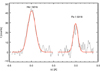 |
Fig. 2. Observed line profiles of He-singlet 5016 Å and Fe II 5018 Å together with the Gaussian fits. Between both lines, ≈2 Å are cut out to stretch the λ scale. |
3. Results
The mean value of the total emission of Hγ observed at the four slit positions amounts to  erg (s cm2 ster)−1, for which Gouttebroze et al. (1993) gave τγ = 0.5, τα = 10.1 and
  erg (s cm2 ster)−1 (table for Tkin = 8000 K, P = 0.2 dyn cm−2 and Δz = 5000 km). Such a high Balmer brightness is a necessary condition for observing weak optically thin metal lines with sufficient accuracy. Since the total emissions of the metal lines are 60−200 times weaker than for Hγ, they can be assumed to be optically thin. Indeed, Landman (1981) obtained for
  (Na D1) = 4420 erg (s cm2 ster)−1 an optical thickness of τD = 0.1. Our Na D1 emission is eight times weaker and thus τD<0.1.
The broadening of optically thin lines is usually described by a thermal and a nonthermal term,  , where V denotes the line widths Δλw in velocity units:
  (where c is the velocity of light, λ0 the line wavelength, and
  the half width at I0e−1 with σ being the width parameter of the Gaussian fits; see Tandberg-Hanssen 1995). We determine the nonthermal term as the difference
  .
.
In Fig. 3 we plot the mean of the observed quantity  for the four slit positions versus the inverse atomic mass μ−1. To obtain a reference, we calculated a linear fit through all lines using the mean values over the scan positions. The corresponding line is displayed in Fig. 3 in dashed orange. From this fit, we subtracted the value at μ−1 = 0 and obtain the solid orange line that we use as reference for the nonthermal broadening. This line represents the pure thermal dependence for 8300 K. With respect to this reference, the line widths of metals deviate significantly. For Sr II, Fe II, and Mg b2 we find nonthermal widths rather similar to those of Ramelli et al. (2012). However, we obtain significant Vnth for Na D1, which those authors did not find for Na D2. We attribute this discrepancy to the terrestrial H2O blend in the Na D2 wing which diminishes the line width (see Wiehr et al. 2019). Hγ and He I also appear above the reference line. For Hγ we had to take into account an additional broadening due to opacity, which we estimated from the tables by Gouttebroze et al. (1993) for 8000 K to be (10 ± 3)%. The reduced V is given by the orange bar in Fig. 3.
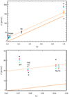 |
Fig. 3. Upper panel: Observed mean values of V2=(c·Δλw/λ0)2 versus the inverse atomic mass 1/μ for the four slit positions marked in Fig. 1. The dotted orange line represents a linear fit through all lines, and the solid orange line is used as reference for width excesses of the spectral lines. The diamonds for Fe II(b) and Mg b separate the close Fe II(a) and Na D values. The orange bar indicates the uncertainty of the opacity broadening of Hγ. Lower panel: Enlargement of the range of the metal lines. The position of Fe II(a) is slightly shifted to separate it from Fe II(b). |
In Fig. 4, we plot, for the metal lines, the deviations of the observed widths from the reference line in Fig. 3 in velocity units,  , versus the inverse atomic mass, μ−1, (as in Fig. 3) and find a range of 3.5<Vnth<6.0 km s−1. Mean values are listed in the last column of Table 1.
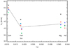 |
Fig. 4. Deviation of the observed widths of metal lines from the reference line in Fig. 3 in velocity units |

4. Discussion and conclusions
The nonthermal line broadening reflects small-scale motions that, in contrast to line shift data, are independent of the line-of-sight angle and presumed to result from interaction with the magnetic field (Parenti et al. 2024). The observation of weak metal lines allows to study the bright prominence body without the influence of optical thickness. The line width excesses that are ultimately obtained are thus not restricted to the prominence border as for strong chromospheric lines. Our lines, however, are too weak for a study of the periphery, only giving sufficient signal at the bright prominence center.
The most prominent result from our study is the almost equal broadening excess of lines from ionized Fe and neutral Na and Mg. For Mg b2 this result confirms the findings of Ramelli et al. (2012) who argue that triplet systems are populated via ionization and recombination. During the intermediate state as ion, magnetic influences modify the velocity distribution. We interpret the broadening of neutral metals by a kind of “ionization memory” occurring after recombination if the line emission happens before a collision changes the momentum of the atom. To get an idea about collision times in the prominence plasma, we used the equation for the free path length
where n is the particle density and r the mean radius of the colliding atoms (Gerthsen & Kneser 1971, p. 64). The particle density of hydrogen was taken from Gouttebroze et al. (1993) for parameters T = 8000 K, p = 0.2 dyn cm−2, and Δz = 5000 km which fit our observed  (see Table 1) Atomic radii were given by Clementi et al. (1967), and we took ionic radii from www.webelements.com. These values concern the ground state, but since emitting atoms are excited, we enlarged the radii by a factor of two as a coarse estimate. We considered collisions of the investigated metals with neutral hydrogen and helium and neglected all other species because they are less frequent, and the protons are much smaller, thus they contribute only a little. Dividing this length by the typical velocity of the colliding particles, we obtain the mean collision time, tc. Such velocities vary between 4 and 10 km s−1 for metals (see Fig. 3), resulting in 10−3 s<tc<10−1 s. A detailed overview is given in Table 2. The widths of the metal lines indicate that each emitter has its individual broadening sensitivity, depending on the time interval between recombination and line emission. The neutral metals apparently have a memory of their previous period as ions and maintain their velocity distribution after recombination. This becomes plausible comparing the mean emission time after recombination (10−9–10−6 s; see Table 1) and the mean collision time (10−4–10−1 s). Although the collision times are approximative, the differences of a few orders of magnitude to the emission times justify our suggestion of an “ionization memory”.
Free path lengths and mean collision times for the different ions.
Concerning the large line broadening excess of Na D1 (not observed by Ramelli et al. 2012), Landman (1981, 1983) argued that sodium is mostly ionized (see ionization potentials in Table 1). A short time after recombination the D lines are emitted. The mean time span between recombination and emission is given in Table 1. So, magnetic forces have influenced sodium during its previous existence as ion.
The highest broadening excess is found for Sr II in agreement with Ramelli et al. (2012). Strontium may be particularly sensitive to magnetic influences since it exists, according to the low second ionization potential in Table 1, most of the time as Sr iii (see Landman 1983). (We note that the Sr II line widths are not affected by isotopy shifts which, according to Heilig 1961, amount to about 1 mÅ.)
In the magnetic field, ions experience the Lorentz force, according to the equation

where q is the electric charge, B the magnetic field, v the velocity, and k is a prefactor. The Lorentz force causes gyration of an ion around the magnetic field lines with the speed of the component of v perpendicular to the magnetic field, but not a linear acceleration of the ion. In the corresponding plane, all directions occur, and in the consequence we observe a broadening of the spectral lines (see also Ballester et al. 2018). Another broadening effect arises when the velocity component along the magnetic field is nonzero and the magnetic field is not perpendicular to gravity direction everywhere, for example in the magnetic field configuration suggested by Kippenhahn & Schlüter (1957). Then a pendulate motion of the ion around the local height minimum of the field lines can occur causing a broadening of the emission lines. Different types of waves also influence the line broadening as well as instabilities or shocks and motions in twisted flux tubes. Such effects are discussed in detail by Ballester et al. (2018). Prominences typically consist of thin threads that are not resolved in our data due to our long exposure times. These threads can move against each other causing a line broadening.
The observed fact that lines from metal emitters are broader than expected from our reference line (see Fig. 3) suggests that the metal emissions are broadened by nonthermal effects. The observed mean Sr II line width would require unlikely high Tkin = 175 000 K if only thermally broadened. Since the observed line profiles are almost perfect Gaussians, we can assume a Maxwellian distribution of nonthermal motions. The helium line also is broader than our reference line, indicating a nonthermal broadening. This can be due to collisions on a longer time scale than the mean emission time. Because of the high ionization potential, only a small fraction of helium atoms will be ionized (see Labrosse & Gouttebroze 2001). The excitation of the helium singlet system is then caused mainly by absorption of exteme ultraviolet radiation (λλ 584 Å and 537 Å) from the chromosphere, followed in the first case by emission of a 2 μm photon and absorption of a photospheric photon (λ 5016 Å). In contrast, for the triplet system, photoionization and recombination play an important role.
Detailed physical processes behind such non-thermal broadening remain still unclear. They are assumed to be of magnetic origin (Parenti et al. 2024). Instabilities at the prominence-corona border can be excluded because our data refer exclusively to the prominence bulge. Since lines from neutral emitters seem to be broadened according to their intermediate existence as ions, a description by a “charged-uncharged” dual scenario will not be sufficient.
Acknowledgments
We are indepted to M. Verma and O. Steiner for carefully reading and commenting the manuscript. We thank B. Gelly and D. Laforgue for assistance with the instrument. THEMIS is operated by the French Centre National de la Recherche Scientifique in the Spanish Observatorio del Teide, Tenerife. E.W. and H.B. received financial support from the European Union's Horizon 2020 research and innovation program under grant agreement No. 824135 (SOLARNET).
References
- Ballester, J. L., Alexeev, I., Collados, M., et al. 2018, Space Sci. Rev., 214, 58 [Google Scholar]
- Clementi, E., Raimondi, D. L., & Reinhardt, W. P. 1967, J. Chem. Phys., 47, 1300 [Google Scholar]
- Gerthsen, C., & Kneser, H. O. 1971, Physik. Elfte berichtigte Auflage (Berlin, Heidelberg, New York: Springer-Verlag) [Google Scholar]
- Gilbert, H. R., Hansteen, V. H., & Holzer, T. E. 2002, ApJ, 577, 464 [NASA ADS] [CrossRef] [Google Scholar]
- Gilbert, H., Kilper, G., & Alexander, D. 2007, ApJ, 671, 978 [Google Scholar]
- González Manrique, S. J., Khomenko, E., Collados, M., et al. 2024, A&A, 681, A114 [NASA ADS] [CrossRef] [EDP Sciences] [Google Scholar]
- Gouttebroze, P., Heinzel, P., & Vial, J. C. 1993, A&AS, 99, 513 [NASA ADS] [Google Scholar]
- Heilig, K. 1961, Z. Phys., 161, 252 [Google Scholar]
- Heinzel, P., Gunár, S., & Jejčič, S. 2024, Phil. Trans. R. Soc. London Ser. A, 382, 20230221 [Google Scholar]
- Khomenko, E. 2017, Plasma Phys. Control. Fusion, 59, 014038 [NASA ADS] [CrossRef] [Google Scholar]
- Khomenko, E., Collados, M., & Díaz, A. J. 2016, ApJ, 823, 132 [Google Scholar]
- Kippenhahn, R., & Schlüter, A. 1957, Z. Astrophys., 43, 36 [Google Scholar]
- Kramida, A., Ralchenko, Y., Nave, G., & Reader, J. 2018, APS Meeting Abstracts, 2018, M01.004 [Google Scholar]
- Labrosse, N., & Gouttebroze, P. 2001, A&A, 380, 323 [NASA ADS] [CrossRef] [EDP Sciences] [Google Scholar]
- Landman, D. A. 1981, ApJ, 251, 768 [Google Scholar]
- Landman, D. A. 1983, ApJ, 269, 728 [Google Scholar]
- Neckel, H., & Labs, D. 1984, Sol. Phys., 90, 205 [Google Scholar]
- Parenti, S., Luna, M., & Ballester, J. L. 2024, Phil. Trans. R. Soc. London Ser. A, 382, 20230225 [Google Scholar]
- Pontin, D. I., Peter, H., & Chitta, L. P. 2020, A&A, 639, A21 [NASA ADS] [CrossRef] [EDP Sciences] [Google Scholar]
- Ramelli, R., Stellmacher, G., Wiehr, E., & Bianda, M. 2012, Sol. Phys., 281, 697 [NASA ADS] [CrossRef] [Google Scholar]
- Soler, R., & Ballester, J. L. 2022, Front. Astron. Space Sci., 9, 789083 [Google Scholar]
- Stellmacher, G., & Wiehr, E. 2015, A&A, 581, A141 [NASA ADS] [CrossRef] [EDP Sciences] [Google Scholar]
- Stellmacher, G., & Wiehr, E. 2017, Sol. Phys., 292, 83 [NASA ADS] [CrossRef] [Google Scholar]
- Tandberg-Hanssen, E. 1995, The Nature of Solar Prominences, Astrophysics and Space Science Library (Dordrecht: Kluwer Academic Publishers), 199 [Google Scholar]
- Wiehr, E., Stellmacher, G., & Bianda, M. 2019, ApJ, 873, 125 [Google Scholar]
- Wiehr, E., Stellmacher, G., Balthasar, H., & Bianda, M. 2021, ApJ, 920, 47 [NASA ADS] [CrossRef] [Google Scholar]
- Zapiór, M., Heinzel, P., & Khomenko, E. 2022, ApJ, 934, 16 [CrossRef] [Google Scholar]
All Tables
All Figures
|
Fig. 1. Hα image of the prominence at the west limb, 52° north, from June 6, 2022, (GONG archive); North direction is upward; the long lines mark the direction of refraction at two slit positions beside the prominence used for the determination of parasitic light; the short lines mark slit positions reconstructed from the observed Hγ intensity variation and their extension of 12″ corresponds to 8.7 Mm. |
| In the text | |
|
Fig. 2. Observed line profiles of He-singlet 5016 Å and Fe II 5018 Å together with the Gaussian fits. Between both lines, ≈2 Å are cut out to stretch the λ scale. |
| In the text | |
|
Fig. 3. Upper panel: Observed mean values of V2=(c·Δλw/λ0)2 versus the inverse atomic mass 1/μ for the four slit positions marked in Fig. 1. The dotted orange line represents a linear fit through all lines, and the solid orange line is used as reference for width excesses of the spectral lines. The diamonds for Fe II(b) and Mg b separate the close Fe II(a) and Na D values. The orange bar indicates the uncertainty of the opacity broadening of Hγ. Lower panel: Enlargement of the range of the metal lines. The position of Fe II(a) is slightly shifted to separate it from Fe II(b). |
| In the text | |
|
Fig. 4. Deviation of the observed widths of metal lines from the reference line in Fig. 3 in velocity units |
| In the text | |
Current usage metrics show cumulative count of Article Views (full-text article views including HTML views, PDF and ePub downloads, according to the available data) and Abstracts Views on Vision4Press platform.
Data correspond to usage on the plateform after 2015. The current usage metrics is available 48-96 hours after online publication and is updated daily on week days.
Initial download of the metrics may take a while.