| Issue |
A&A
Volume 695, March 2025
|
|
|---|---|---|
| Article Number | A235 | |
| Number of page(s) | 19 | |
| Section | Galactic structure, stellar clusters and populations | |
| DOI | https://doi.org/10.1051/0004-6361/202453227 | |
| Published online | 21 March 2025 | |
Multi-wavelength characterization of VVVX open clusters
1
Instituto de Astronomía, Universidad Católica del Norte,
Av. Angamos 0610,
Antofagasta,
Chile
2
ESO – European Southern Observatory,
Alonso de Cordova 3107,
Vitacura, Santiago,
Chile
3
Instituto de Astrofísica, Depto. de Ciencias Fisicas, Facultad de Ciencias Exactas, Universidad Andrés Bello,
Av. Fernández Concha 700,
Las Condes, Santiago,
Chile
4
Vatican Observatory,
V00120 Vatican City State,
Italy
5
Observatorio Astronómico, Universidad Nacional de Córdoba,
Laprida 854, X5000BGR Córdoba,
Argentina
6
Instituto de Astronomía Teórica y Experimental (CONICET-UNC),
Laprida 854, X5000BGR Córdoba,
Argentina
7
Departamento de Matemática, Facultad de Ingeniería, Universidad de Atacama,
Copiapó,
Chile
★ Corresponding authors; This email address is being protected from spambots. You need JavaScript enabled to view it.
; This email address is being protected from spambots. You need JavaScript enabled to view it.
Received:
29
November
2024
Accepted:
17
February
2025
Abstract
Context. With the rise of large surveys across wavelengths, both supervised and unsupervised machine learning algorithms have increasingly aided in detecting large samples of old open clusters in high-extinction regions of the Milky Way bulge and disk.
Aims. Our primary goal is to confirm or discard automatically detected open clusters from poorly studied, heavily contaminated regions of the Milky Way. Cleaning these samples is critical for reconstructing the Galactic disk’s star formation history and understanding the thin and thick disk formation model.
Methods. We used data from the VVVX, 2MASS, and Gaia DR3 surveys to confirm and characterize nine open cluster candidates: BH118, BH 144, Schuster-MWSC 1756, Saurer 3, FSR 1521, Saurer 2, Haffner 10-FSR 1231, Juchert 12, and Pismis 3. We constructed density maps and vector–proper motion diagrams to analyse the targets and performed photometric analysis to derive their main physical parameters.
Results. We examined cluster images from the 2MASS, WISE, and DECaPS surveys, identifying star clusters through an over-density of stars. This was confirmed with a VVVX photometry density map and validated using Gaussian kernel density estimation. Using Gaia proper motion data, we refined cluster memberships and decontaminated the data to build the final cluster catalogue with objects with a high probability of being star cluster members. We derived the following parameters: extinction values (AKs) ranging from 0.07±0.03 to 0.50±0.04; colour excess values (E(J-Ks)) from 0.16±0.03 to 0.60±0.03; distances (D) from 2.19±0.06 kpc to 8.94±0.06 kpc; Galactocentric distances (RG) from 7.82 kpc to 15.08 kpc; vertical distance component values (Z) from −0.09 kpc to 0.34 kpc; and tangential velocities (VT) from 30.59 km/s to 245.42 km/s. We also computed ages and metallicities by fitting PARSEC isochrones, finding ages (t) ranging from 20 Myr to 5 Gyr and metallicities ([Fe/H]) from −0.5 to 0.5. Structural parameters include core radii (rc) from 0.71′ to 5.21′, tidal radii (rt) from 3.4′ to 12.0′, and concentration indices (c) from 0.36 to 0.83.
Conclusions. We photometrically confirm the open cluster nature for the nine targets in our compilation and updated their main physical parameters.
Key words: Galaxy: bulge / Galaxy: disk / Galaxy: formation / Galaxy: general / open clusters and associations: general
© The Authors 2025
 Open Access article, published by EDP Sciences, under the terms of the Creative Commons Attribution License (https://creativecommons.org/licenses/by/4.0), which permits unrestricted use, distribution, and reproduction in any medium, provided the original work is properly cited.
This article is published in open access under the Subscribe to Open model. This email address is being protected from spambots. You need JavaScript enabled to view it. to support open access publication.
1 Introduction
In the last three decades, interest in the studies of intermediate-age (100 Myr–1 Gyr) and old (>1 Gyr) Galactic open clusters (OCs) has increased significantly (see e.g. Montgomery et al. 1994; Phelps 1994; Friel 1995; Tosi et al. 1998; Frinchaboy et al. 2004; Tosi et al. 2007; Friel et al. 2010; Angelo et al. 2019; Tarricq et al. 2022). The reason is that understanding their properties, such as ages, metallicities, and kinematics, is fundamental to better discerning the structure and formation history of the thin and thick disk (Carraro & Chiosi 1994).
In the era of extensive surveys, such as the Two Micron All-Sky Survey (2MASS; Skrutskie et al. 2006) and Gaia (Gaia Collaboration 2016), there has been an explosion in the discovery of OCs. From Sloan Digital Sky Survey (SDSS; York et al. 2000) and 2MASS images of selected Milky Way regions, Kronberger et al. (2006) discovered 66 stellar groupings. The morphologies, colour–magnitude diagrams (CMDs), and stellar density distributions of these objects suggest they are potential OCs, and none of them have previously been listed in any catalogue. Kronberger et al. (2006) provided extensive descriptions for 24 candidates considered the most likely OCs based on 2MASS photometry. Of these 24, only 9 objects had fundamental parameters determined by fitting the CMDs with solar-metallicity Padova isochrones (Marigo et al. 2017). An additional 10 cluster candidates had distance moduli and reddenings derived from Ks magnitudes and colour indices of helium-burning red clump (RC) stars.
The Kharchenko et al. (2013) catalogue identified 3006 real objects from an initial list of 3784 targets obtained from various sources. While most of these objects are classified as OCs, the catalogue also includes stellar associations and globular clusters. It provides essential cluster parameters such as the central position, apparent size, proper motion (PM), distance, colour excess, and age. However, 778 of the 3006 objects were not confirmed as real objects.
In another study, Cantat-Gaudin et al. (2020) identified 2000 clusters using Gaia Data Release (DR) 2 astrometry. Using deep Gaia photometry down to G=18, they measured the distance, age, and reddening of these clusters. An artificial neural network, trained on previously documented objects with well-defined parameters, was employed to estimate the parameters of these new clusters. Out of the 2000 clusters analysed, reliable parameters were obtained for 1867.
The VISTA Variables in the Via Láctea extended Survey (VVVX) has played a central role in confirming many new globular clusters and OCs within the Galactic bulge and central region, where spatial extinction is high (Saito et al. 2024; Obasi et al. 2023, 2024; Garro et al. 2022a,b, 2024). Recently, we utilized VVVX data to discover and characterize a new OC, Garro 3 (Garro et al. 2024).
Recent OC studies have also relied heavily on the Gaia survey; for example, 628 OCs were discovered by Castro-Ginard et al. (2022) using the OC finder algorithm with Gaia Early Data Release 3 (EDR3) data, and 704 new potential clusters were found by Hao et al. (2022) using the sample-based clustering search method and Gaia EDR3 data. A machine-learning approach was developed using Gaia data and 23 new OCs in the Tycho-Gaia Astrometric Solution dataset (Castro-Ginard et al. 2018). Cantat-Gaudin et al. (2019) found 41 new OCs towards the Perseus Arm and 53 new OCs towards the Galactic anti-centre. These are just a few of the newly discovered OCs. However, the physical parameters of many detected but unconfirmed clusters have not yet been characterized.
Consequently, many new findings are considered potential OC candidates, and some are determined false positives once better observations are made. For example, FSR 1333, with J2000 coordinates α = 123.108, δ = −27.9130, and FSR 1651, with J2000 coordinates α = 201.382, δ = −58.9850, were both classified as OCs by Buckner & Froebrich (2013). However, our analysis using VVVX data reveals no over-density in the VVVX photometry density map or Gaussian kernel density estimation (KDE), as shown in Fig. 1. This suggests that both might be false positive detections.
Therefore, it remains essential to confirm these new detections and measure their physical parameters. In this context, one of the primary objectives of the VISTA Variables in the Via Láctea (VVV) team is to confirm new star clusters within the VVV survey (Minniti et al. 2010; Saito et al. 2012) and its extension VVVX (Saito et al. 2024) based on observations at the 4 m Visible and Infrared Survey Telescope for Astronomy (VISTA). The strength of the VVV lies in its near-infrared (NIR) operating wavelength, which has proven to be much more effective in the highly crowded central region of the Galactic bulge where high spatial extinction exists.
We used a combination of VVVX, 2MASS, and optical Gaia DR3 (Gaia Collaboration 2021) data (listed in Table 1) to confirm and characterize the physical nature of nine selected OCs towards the Galactic bulge. Additionally, we provide the first physical measurements and characterization of Jurchert12. Section 2 describes the datasets used in this work. Section 3 outlines the methodology for the analysis. In Sect. 4, we present our derived physical parameters and a summary of the results. Section 5 presents the results in more detail, while Sects. 6 and 7 present the discussion and conclusions.
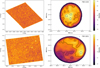 |
Fig. 1 VVVX density maps and Gaussian KDEs for the clusters FSR 1333 (upper panels) and FSR 1651 (lower panels). |
2 Datasets
We used VVVX data in combination with 2MASS and Gaia DR3 to characterize nine OC candidates – BH118, BH144, Schuster-MWSC1756, Saurer 3, FSR1521, Saurer 2, Haffner10FSR1231, Juchert12, and Pismis3 – listed in the catalogues of Kronberger et al. (2006), Kharchenko et al. (2013), and Cantat-Gaudin et al. (2020). These clusters had not been properly characterized before. Our datasets comprise both NIR and optical data, and we used a matching radius of 0.5″. The NIR data came from the VVVX and the 2MASS (Saito et al. 2024; Skrutskie et al. 2006). The VVVX is a public ESO survey, conducted with the VISTA Infrared Camera (VIRCAM) on the 4.1 m VISTA telescope (Emerson & Sutherland 2010).
The point spread function photometry was extracted as described by Alonso-García et al. (2018). Astrometry was calibrated to the Gaia DR3 (Gaia Collaboration 2021) reference system, while photometry was calibrated to the VISTA magnitude system (González-Fernández et al. 2018) against the 2MASS using a globally optimized model of frame-by-frame zero points plus an illumination correction. We used NIR 2MASS data to reach magnitudes brighter than Ks = 11, which are saturated in the VVVX images. Although we treated the VVVX and 2MASS data separately, we scaled them to the same photometric system (González-Fernández et al. 2018), applying correction offsets of ΔKs < 0.009 and ΔJ < 0.050.
Previous studies on these clusters by Kronberger et al. (2006), Kharchenko et al. (2013), and Cantat-Gaudin et al. (2020) have produced conflicting results, with no generally agreed-upon properties. The inspection of the VVVX tiles that contain these clusters revealed a clear and well-separated over-density of red giant stars at their equatorial coordinates, listed in Table 1. This confirms their status as real star clusters. Additionally, we visually inspected all the cluster overdensities in the 2MASS, Wide-field Infrared Survey Explorer (WISE), and Dark Energy Camera Plane Survey (DECaPS) images to ensure that these features were not artefacts and remained consistent under small variations of parameters (i.e. observing the targets in different wavelengths).
Cluster name, coordinates (RA and Dec), Galactic coordinates (l and b), VVVX tile corresponding to each cluster, and literature references.
3 Methodology
To achieve the objectives of this study, we followed methods similar to those outlined in Obasi et al. (2021) and Garro et al. (2022b). We began our investigation by carefully examining images captured at various wavelengths, as shown in Figs. 2 and A.4. The first and third panels display cluster images captured at various wavelengths. In all three images in the first and third panels, there is clear evidence of stellar over-densities, which resemble star clusters published in the literature. However, additional checks are required to validate our initial assumption since these overdensities are observed in a densely populated region.
First, we created a density map using VVVX photometry for the tiles corresponding to each cluster with the TOPCAT program (Taylor 2005), revealing a clear excess of stellar density at the cluster location, as shown in the left panels of Figs. 2 and A.4 (second and fourth panels). Starting from the cluster locations in each tile, we applied cone selection and then performed KDE on the resulting data to examine the clusters’ overdensities in more detail. This statistical method enables a more accurate distinction between stellar overdensities and background fluctuations, beyond simple visual inspection. The KDE analysis confirmed a centralized, circular overdensity, as shown in the right panels of Figs. 2 and A.4 (second and fourth panels). These tests provide compelling evidence that these objects are indeed star clusters.
3.1 Decontamination procedure and cluster membership
Studying the inner region of the Milky Way, such as the bulge and disk, is always challenging. Several factors contribute to these difficulties, such as differential reddening and extinction. These factors not only impact the accuracy of photometric distance estimates but also influence derived cluster parameters such as age and metallicity. To mitigate some of these challenges, we applied the following cuts: π < 0.5″ (parallax to avoid severe contamination from foreground stars) and renormalized unit weight error (ruwe) <1.4 (a high-quality astrometric parameter). This ensures that the photometric data all have reliable astrometric solutions that are consistent with our previous studies (Garro et al. 2022b, 2024). We then used KDE isodensity contours (Figs. 2 and A.4 second and fourth right panels) to statistically show the significance of the stellar overdensity and eliminate false positives masquerading as genuine stellar overdensities as we previously demonstrated in Fig. 1. This method is also similar to our analysis in the previous paper (Garro et al. 2024). To refine our sample and eliminate contaminants, we computed the membership probability for each cluster. Accurate membership determination is crucial for deriving the clusters’ astrophysical parameters. Vasilevskis et al. (1958) introduced the first mathematical model for membership determination, which was later refined by Sanders (1971) using the maximum likelihood principle. Since then, improved methods for determining star membership in clusters based on PMs and different observed precisions have been developed (see Stetson 1980; Zhao & He 1990; Zhao & Shao 1994). We first applied a Gaussian mixture model with two components to the PM data in right ascension (RA) and declination (Dec) to determine cluster membership probabilities, effectively separating cluster stars from field stars. For each group, we calculated the mean and standard deviations of μα* and μδ. Furthermore, the separation of the two distributions (D) was quantified by comparing their means μ1 and μ2, normalized by their standard deviations σ1 and σ2. Using D, we could measure the distance between the centres of two distributions and thereby determine whether the two distributions overlap or not. Our clusters have a minimum D value of 2.5, consistent with the threshold noted by Muratov & Gnedin (2010) and Ashman et al. (1994), who suggest that a clean separation between modes requires D>2. Figure 3 presents a histogram of the cluster and field distributions for BH144, clearly illustrating the distinct separation of the cluster mean from the field.
We applied a straightforward yet effective method for estimating membership probabilities and identifying probable cluster members based on PMs, closely following the approach of Sanders (1971). We began by defining the PMs (Mxi, Myi) as well as their mean values (Mxc, Myc), obtained by using the Gaussian mixture model code, along with their uncertainties (EMxi, EMyi). σc represents the PM radius of the cluster. The normalized factor, (factor1), is defined as
![Mathematical equation: $\[\text{factor1} =\sqrt{2 \pi} \cdot \sqrt{\left(\sigma_{c}^{2}+E_{M_{x i}}^{2}\right)\left(\sigma_{c}^{2}+E_{M_{y i}}^{2}\right)}.\]$](/articles/aa/full_html/2025/03/aa53227-24/aa53227-24-eq1.png) (1)
(1)
Next, we calculated the squared distance between each star’s PM and the cluster mean:
![Mathematical equation: $\[\begin{aligned}& n_x^2=\left(M_{x i}-M_{x c}\right)^2 \\& n_y^2=\left(M_{y i}-M_{y c}\right)^2.\end{aligned}\]$](/articles/aa/full_html/2025/03/aa53227-24/aa53227-24-eq2.png) (2)
(2)
The variances for pmra and pmdec were defined as
![Mathematical equation: $\[\begin{aligned}& \sigma_{n x}^2=\sigma_c^2+E_{M_{x i}}^2 \\& \sigma_{n y}^2=\sigma_c^2+E_{M_{y i}}^2.\end{aligned}\]$](/articles/aa/full_html/2025/03/aa53227-24/aa53227-24-eq3.png) (3)
(3)
We then computed the exponential component, known as factor2, for the membership probability:
![Mathematical equation: $\[\text{factor2}=\exp \left(-\frac{1}{2}\left(\frac{n_{x}^{2}}{\sigma_{n x}^{2}}+\frac{n_{y}^{2}}{\sigma_{n y}^{2}}\right)\right).\]$](/articles/aa/full_html/2025/03/aa53227-24/aa53227-24-eq4.png) (4)
(4)
The un-normalized membership probability, pf, was calculated as
![Mathematical equation: $\[p_{f}=\frac{\text { factor} 2}{\text { factor} 1}.\]$](/articles/aa/full_html/2025/03/aa53227-24/aa53227-24-eq5.png) (5)
(5)
For clarity, we normalized the membership probabilities to a maximum of 1. This normalization resulted in a clear distinction between cluster members and interlopers, defined by
![Mathematical equation: $\[\operatorname{pdf}=\frac{p_{f}}{\max \left(p_{f}\right)}.\]$](/articles/aa/full_html/2025/03/aa53227-24/aa53227-24-eq6.png) (6)
(6)
We set our membership threshold T to classify stars as follows:
![Mathematical equation: $\[\text { Membership Status }=\left\{\begin{array}{ll}\text { Member } & \text { if } p_f \geq T \\\text { Non-Member } & \text { if } p_f<T\end{array}.\right.\]$](/articles/aa/full_html/2025/03/aa53227-24/aa53227-24-eq7.png) (7)
(7)
Our selection criteria were strict, with T typically set to ≥0.9 in most cases. Figure 4 shows the magnitude versus membership probability plot for cluster BH 144. The red dotted horizontal line indicates a 90% confidence level that a star belongs to the cluster.
Subsequently, we constructed the CMD for all the clusters in both the 2MASS NIR and optical Gaia data. In eight cases, distinct RC stars are seen, as observed in Fig. 5 for the cluster Pismis3. We measured the mean position of the RC overdensity using KDE to compute the max_density_index indicated by the dotted horizontal line and their corresponding error. For the clusters listed in Table 1, we present in Table 2 their Ks and J-Ks for the RC.
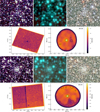 |
Fig. 2 Top panel: multi-band images of the OC BH118 from 2MASS (left), WISE (middle), and DECaPS (right). Second panel: cluster density map highlighting the darkest region as the cluster location (left) and the KDE distribution (right). Third and fourth panels: same but for BH144. |
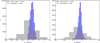 |
Fig. 3 Histograms of PMs (μα* and μδ), highlighting the distributions of the cluster (blue) and field (grey) populations along with their respective mean values. |
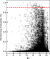 |
Fig. 4 Membership probability as a function of Ks magnitude. The dashed horizontal line indicates the 90% cluster membership threshold for BH144. |
4 Estimation of the main physical parameters
We used the final catalogue obtained from our decontamination process for the rest of the analysis. We derived distance, reddening, and extinction. We built CMDs of the clusters and derived astrophysical parameters such as age and metallicity. The use of multiband photometry in our analysis, comprising VVVX+2MASS and optical Gaia data, helped us obtain more robust results. Structural parameters, such as the core radii, tidal radii, and concentration parameters, are presented in the next subsections.
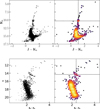 |
Fig. 5 Upper panel: 2MASS NIR CMD (Ks vs J-Ks). On the right, the RC overdensity is visible on the density map, and the horizontal line indicates the density peak. Lower panel: same but with optical Gaia data (G vs BP-RP) for Pismis3. |
Values of Ks and J − Ks for the RC.
4.1 Reddening, extinction, distance, vertical component, and tangential velocity
We computed the reddening and extinction associated with each cluster we studied. To do this, we followed the method outlined by Ruiz-Dern et al. (2018), as we have done in our previous studies (Obasi et al. 2021; Garro et al. 2022b). We used two methods to verify the position of the RC stars in each cluster. First, we built the CMD (J vs J-Ks) and used KDE to estimate the positions of Ks and J-Ks as demonstrated in Fig. 5 (upper panel). We then verified the consistency of this method by constructing the generic luminosity function in the Ks band for each cluster, finding that the values obtained were in agreement.
Three methods were used to calibrate the extinction and reddening in our sample. First, we used Schlafly & Finkbeiner (2011) and Cardelli et al. (1989) to determine the extinction and reddening values. Second, we applied the extinction law from Nataf et al. (2015). Third, we calibrated our extinction and reddening values using the absolute magnitude of RC stars in the Ks band (MKs = −1.605 ± 0.009) and their intrinsic colour ((J − Ks)0 = 0.66 ± 0.02) from Ruiz-Dern et al. (2018). Based on these methods, we reported only the values from Nataf et al. (2015) and Ruiz-Dern et al. (2018), as they showed excellent agreement in their derived distances. We adopted the Ruiz-Dern et al. (2018) extinction law for the corrections. In Sect. 6 we briefly discuss the reasons for the differences between these results and the exclusion of Schlafly & Finkbeiner (2011).
For the young cluster Haffner 10, whose CMD lacks a well-populated red RC sequence due to its age (~20 Myr), we applied the extinction law derived by Nishiyama et al. (2009, AKs = 0.67· E(J - Ks) to compute both extinction and reddening. The derived extinction for all the clusters varied widely, ranging from AKs = 0.07±0.03 to 0.50±0.04, and the reddening ranged from E(J-Ks)0=0.16±0.03 to 0.60±0.03. Using these values, we estimated the heliocentric distances of the clusters by applying the distance modulus equation. For Haffner 10, we first computed its distance using Gaia parallaxes. The two methods yielded similar distance results for each cluster; therefore, we adopted and reported the average values in Table 4, which range from D = 2.19±0.06 kpc to D = 8.94±0.06 kpc.
We adopted R⊙ = 8.2 kpc (Abuter et al. 2019) to compute the Galactocentric distance, which ranged from RG = 7.82 kpc to 15.08 kpc. Using the relation Z = D×sin(b), assuming Z⊙ = 0.007 kpc (Siegert 2019), we estimated the distance to the Galactic plane for each cluster, which ranged from Z = −0.09 kpc to 0.34 kpc, both below and above the Galactic plane. Finally, we computed the tangential velocities of each cluster, which ranged from VT = 30.59 km/s to 245.42 km/s. This kinematic parameter allowed us to deduce the Galactic component each of the clusters belongs to, which we discuss further in the following section.
4.2 Ages and metallicities
Following a similar procedure to our previous work (Obasi et al. 2021) and taking into account our derived reddening values, extinctions, and distances for each cluster, we fitted PARSEC isochrones (Bressan et al. 2012). We visually inspected the fit until a match was obtained. Age and [Fe/H] were then obtained from this procedure.
We fixed the reddening and distance values estimated from the RC stars and fit the isochrones for different ages and metallicities. To derive robust fits, we varied the age and metallicity until an optimal match was found. This method reliably constrained the age and [Fe/H] for each cluster, as demonstrated in Sect. 6, where we discuss our results and compare them to values in the literature. The best-fitted isochrones in the VVVX and Gaia CMDs are shown in Figs. 7 and A.5–A.8. The best-fitted parameters are listed in Table 4. The uncertainties in metallicities and distances in our study are estimated to be approximately 0.5 dex in ages and 0.2 dex in metallicities, consistent with findings from similar studies on OCs (e.g. Garro et al. 2024; Saroon et al. 2024).
4.3 Structural parameters
We measured the physical size of the clusters following a similar approach used by Obasi et al. (2021). First, we computed the radial density profile (RDP). The initial centre coordinates obtained from the literature for each cluster were recomputed. The new centre was determined by calculating the median values of μα and μδ within a radius of 0.1′ from the literature values. This newly derived centre was then used to build the RDPs.
For each cluster, we divided our sample into circular annuli with increasing radii moving outwards from the centre. The number density per bin was computed as the number of stars (N) in the bin divided by the area (A). The RDP for each cluster is plotted as a function of the mean distance of the circular annulus from the cluster centre against the number density in the corresponding annuli. The error bars were computed as ![Mathematical equation: $\[e=\sqrt{N / A}\]$](/articles/aa/full_html/2025/03/aa53227-24/aa53227-24-eq8.png) , following the method used in our previous work (Garro et al. 2022b). We subtracted the background level, which varies from 0.3 to 0.8 stars/arcmin2, depending on the cluster.
, following the method used in our previous work (Garro et al. 2022b). We subtracted the background level, which varies from 0.3 to 0.8 stars/arcmin2, depending on the cluster.
To derive the physical parameters of the clusters, we used the model by King (1962) to fit the cluster density profile. From the best-fit parameters, we obtained: the core radius (rc), which ranges from 0.71′ to 5.21′; the tidal radius (rt), which varies from 3.6′ to 12′; and the concentration parameter (c), which ranges from 0.36′ to 0.83′ (see Fig. A.9 for details).
5 Results
We employed a multiwavelength approach using VVVX+ Gaia DR3 and 2MASS+ Gaia DR3 data to improve measurements, resolve inconsistencies from previous literature for eight OCs, and provide a detailed characterization of Jurchert12 for the first time.
We began by deriving the extinction and reddening values for each cluster using the relation provided by Nataf et al. (2015), where AV/AKs = 13.44 and E(J-Ks)/AKs = 0.43. This relation is optimized for the Milky Way’s inner region, where extinction levels are particularly high. The results obtained from this method were compared with those from Ruiz-Dern et al. (2018) to ensure consistency. The AV values for each cluster were retrieved from the NASA/IPAC database1, which uses the relation from Schlafly & Finkbeiner (2011) to compute AV.
For BH118, we find AV = 1.66 ± 0.10 and E(B-V) = 0.53 ± 0.05. For BH144, we find AV = 2.52 ± 0.10 and E(B-V) = 0.81 ± 0.06. The results for the other clusters are presented in Tables 3 and 4.
Next, we applied the extinction and reddening relation by Nataf et al. (2015) to determine each cluster’s NIR extinction and reddening. For BH118, we obtained AKs = 0.12 ± 0.01 and E(J-Ks) = 0.05 ± 0.0. For BH144, we find AKs = 0.19 ± 0.01 and E(J-Ks) = 0.08 ± 0.0. The values for the other clusters are presented in Table 3.
Using these parameters and the absolute MK derived by Alves et al. (2002), MK=−1.61±0.03, we estimated the distance modulus (m − M)0 for each cluster: 14.57 ± 0.03 for BH118 and 14.65 ± 0.05 for BH144. We report the results for other clusters in Table 3.
These values translate to heliocentric distances of 8.20 ± 0.13 kpc for BH118 and 8.53 ± 0.20 kpc for BH144. The results for other clusters are presented in Table 3.
We then validated these values using the Ruiz-Dern et al. (2018) relation. After measuring the RC positions in each cluster. To compute for the extinction, we adopted the relation given in Alonso-García et al. (2017, AKs/(E(J-Ks)=0.428±0.005); we found the following NIR extinction and excess colour values: for BH118, AKs = 0.07 ± 0.03 and E(J − Ks) = 0.16 ± 0.03; for BH144, AKs = 0.07 ± 0.08 and E(J − Ks) = 0.17 ± 0.08. We present the results for the other clusters in Table 3. These values were used to estimate the distance modulus and distances to the clusters, resulting in the following: for BH118, 14.61 ± 0.03 and 8.36 ± 0.03 kpc; for BH144, 14.76 ± 0.11 and 8.95 ± 0.11 kpc. The other clusters’ results are listed in Table 3.
Although extinction and reddening were calculated differently using the methods from Nataf et al. (2015) and Ruiz-Dern et al. (2018), the two approaches yielded very similar distance results. We averaged the distances from these methods (see Table 4) and compared them with those obtained using Gaia data. For Gaia, we used the Babusiaux et al. (2018) relation to compute extinction AG and colour excess Bp-Rp. Since higher extinction affects distance calculations, we only reported distances for clusters with AG < 4. The Gaia distances and the AG value from the Gaia data are presented in Table 4, and the Gaia distances are within 2σ of the other distances. Furthermore, we used the new average distances to calculate the Galactocentric distance RG for each cluster, adopting R⊙ = 8.2 kpc (Abuter et al. 2019). The RG values obtained ranged from 7.82 kpc to 15.08 kpc (see Table 4 for details). Furthermore, we computed the vertical distance Z, which ranged from −0.09 to 0.34 kpc for all clusters. Figure 6 shows the sky distribution of the clusters according to vertical distance (see Table 4 for the complete Z values). In Table 4, the computed PM and tangential velocities for each cluster are also shown.
Finally, using isochrone fitting, we estimated the ages and [Fe/H] values for all clusters. The ages range from 20 Myr to 5 Gyr, while the [Fe/H] values range from −0.5 to 0.5 dex. The results of the isochrone fitting are presented in Table 4. Additionally, we derived structural parameters for the clusters, including core radius (rc), tidal radius (rt), and concentration index (c). The structural parameter values, also shown in Table 4, confirm that all the clusters are genuine OCs and none have undergone core collapse.
Extinction, reddening, distance modulus, and distances for the clusters.
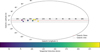 |
Fig. 6 Sky distribution plot of all nine clusters, showing their positions in Galactic coordinates (longitude l and latitude b), with colour representing their tangential velocities. |
6 Discussion
A discussion of our results is presented in this section, along with a comparison of our obtained values with those found in the literature where available. In order to improve previous measurements and study the cluster in detail, we used a multiwavelength approach using VVVX+Gaia DR3 and 2MASS+Gaia DR3. This discussion begins by comparing each object with literature values, followed by an observation of the general trends observed across the sample.
BH118: For the cluster BH118, we obtained AV = 1.66 ± 0.10 and E(B-V) = 0.53 ± 0.05. Cantat-Gaudin et al. (2020), however, reported a lower extinction value of AV = 1.07. Using both Nataf methods and the Ruiz-Dern method for NIR, we obtained the following values: AKs and E(J-Ks) as 0.12 ± 0.01, 0.05 ± 0.003 and 0.07 ± 0.03, 0.16 ± 0.03, respectively. With these parameters, we computed a distance modulus of 14.57 ± 0.03 and 14.61 ± 0.03, equivalent to distances of 8.20 ± 0.13 kpc and 8.36 ± 0.03 kpc for the two methods. Both results are in good agreement with those obtained by Cantat-Gaudin et al. (2020), where (m-M)0 = 14.72 and D = 8.8 kpc. The Galactocentric distance RG of 9.20 kpc we computed for BH118 is consistent with the 9.6 kpc value obtained by Cantat-Gaudin et al. (2020). Additionally, the vertical distance of 0.34 kpc we obtained aligns with the 0.36 kpc reported by Cantat-Gaudin et al. (2020).
Our computed PM values μα = −5.821 ± 0.209 mas yr−1 and μδ = 1.609 ± 0.280 mas yr−1 are in good agreement with those computed by Cantat-Gaudin et al. (2020), which are μα = −4.406 mas yr−1 and μδ = 1.450 mas yr−1. Furthermore, we derived the tangential velocities using these PMs and distances as VTα* ≈ −225.42 km/s and VTδ ≈ 62.31 km/s. These positional and kinematic parameters suggest that BH118 is a disk cluster, as we discuss later in this section. Finally, we derived an age of 3 ± 0.5 Gyr and [Fe/H] = −0.5 dex. However, Cantat-Gaudin et al. (2020) estimated the age of BH118 to be ≈2 Gyr. We over-plotted the isochrone family of 5, 3, and 2 Gyr to the CMD, as shown in Fig. 7. The 3 Gyr isochrone provides a much better fit to the cluster. The core radius (rc), tidal radius (rt), and concentration index (c) of 0.86 ± 0.08′, 5.76 ± 0.92′ (see Fig. A.9), and 0.83, respectively, all indicate a typical OC found in the disk (see Garro et al. 2022b; Saroon et al. 2024).
BH144: For BH144, our derived AV value of 2.52 ± 0.10 is slightly higher than the value provided by Cantat-Gaudin et al. (2020) AV = 1.68. However, our colour excess E(B-V) = 0.81 ± 0.06 is in good agreement with the value of 0.63 obtained by Kharchenko et al. (2013). Using the two methods previously described, we obtained AKs and E(J-Ks) values of 0.19 ± 0.01, 0.08 ± 0.0 and 0.07 ± 0.08, 0.17 ± 0.08, respectively. The distance we computed using the Ruiz-Dern method, 8.95 kpc, agrees with the Cantat-Gaudin et al. (2020) estimation of 9.6 kpc. Furthermore, our computed Galactocentric distance RG = 7.82 kpc aligns with the value calculated by Cantat-Gaudin et al. (2020) of 8.3 kpc. Our calculated vertical distance of −0.49 kpc also agrees with the value of −0.53 kpc reported by Cantat-Gaudin et al. (2020). Our PM values are in excellent agreement with those of Cantat-Gaudin et al. (2020, see our Table 4 for comparison). However, the values computed by Kharchenko et al. (2013) μα = −13.19 mas yr−1 and μδ = 7.74 mas yr−1 largely deviate from our calculations. Similarly, the values provided by Dias et al. (2014) μα = −4.73 mas yr−1 and μδ = −3.36 mas yr−1 also deviate slightly from our values. Our derived tangential velocities for BH144 (see Table 4) suggest that this cluster is located in the disk. Finally, isochrones of 6, 4, and 2 Gyr were utilized, with the best fit at 2 ± 0.2 Gyr and [Fe/H] = 0.5 dex. Kharchenko et al. (2013) estimated an age of 1 Gyr with [Fe/H] = −0.5 dex, while Cantat-Gaudin et al. (2020) derived an age of 1.5 Gyr, consistent with our findings (see Fig. A.5). The structural parameters rc and rt of 1.9 pc and 11.88 pc slightly differ from Kharchenko et al. (2013) values of 0.83 pc and 12.88 pc.
Schuster-MWSC1756: We calculated AV = 10.76 ± 0.10 and E(B-V) = 3.47 ± 0.20 for the cluster Schuster-MWSC1756. In contrast, Kharchenko et al. (2013) calculated a lower colour excess of E(B-V) = 1.08. In Table 3, we report our NIR AKs, E(J-Ks) values, the distance modulus, and cluster distance, while in Table 4 we report the Galactocentric distance based on these parameters.
Our computed PM values are in good agreement with those computed by Cantat-Gaudin et al. (2020, see our Table 4), but they differ significantly from the values obtained by Kharchenko et al. (2013) μ α = −9.41 mas yr−1 and μδ = 3.06 mas yr−1. The tangential velocities suggest that this cluster lies in the disk. Of all the clusters we examined, Schuster-MWSC175 is the smallest size, with core and tidal radii of rc = 1.4 pc and rt = 7.04 pc, respectively (see Fig. A.9). Given the high extinction in this cluster (AV > 10), effective decontamination was challenging, particularly in the Gaia optical CMD. We compared isochrone fits at 400, 700, and 900 Myr with [Fe/H] of −0.5, 0.0 and 0.0 dex (see Fig. A.6); however, the sparsity of the CMD data makes it difficult to precisely determine the cluster’s age, which tends to be 700 Myr. Nevertheless, it appears significantly older than the 6.3 Myr estimated by Kharchenko et al. (2013). For clusters with AV ≥ 5, we did not derive distances using Gaia data, and therefore we did not fit any isochrones on them.
Saurer 3: The E(B-V) = 0.83 ± 0.06 value we obtained for Saurer 3 is consistent with the 0.78 derived by Kharchenko et al. (2013). However, our computed PM values, μ α = −6.62 ± 0.20 mas yr−1 and μδ = 3.24 ± 0.91 mas yr−1, differ from those computed by Dias et al. (2014), who estimated μ α = −6.73 mas yr−1 and μδ = −1.62 mas yr−1. These values are also significantly different from those obtained by Kharchenko et al. (2013), which are μ α = −8.34 mas yr−1 and μδ = 4.40 mas yr−1. Furthermore, our derived age of 2 ± 0.2 Gyr and [Fe/H] = 0.5 dex (see Fig. A.6, bottom panel) aligns closely with the ≈2 Gyr estimate reported by Kharchenko et al. (2013). We also derived structural parameters: a rc of 0.79 ± 0.12′ (corresponding to (rc = 1.6) pc), a rt of 4.65 ± 0.21′ (corresponding to (rt = 9.6 pc), and a concentration index (c) of 0.77. These values are significantly different from those provided by Kharchenko et al. (2013), which are rc = 9.18 pc and rt = 20.46 pc, respectively.
FSR 1521: Cantat-Gaudin et al. (2020) obtained an AV of 2.72, which is about eight magnitudes smaller than the AV = 10.32 ± 0.10 that we obtained for the cluster FSR 1521 using the extinction relation from Schlafly & Finkbeiner (2011). Additionally, our E(B-V) = 3.33 ± 0.20 differs significantly from the 0.37 measured by Kharchenko et al. (2013). These differences between our values and those in the literature might stem from our approach to computing optical extinction, where we use values provided by Schlafly & Finkbeiner (2011).
Our computed (m − M)0 = 12.46 ± 0.03 and distance of 3.10 ± 0.05 kpc agree reasonably well with (m − M)0 = 13.47 and D = 4.9 kpc reported by Cantat-Gaudin et al. (2020). We computed a Galactocentric distance RG = 8.23 kpc, which is consistent with the 8.8 kpc calculated by Cantat-Gaudin et al. (2020). Similarly, our vertical-horizontal distance is consistent with the value provided by Cantat-Gaudin et al. (2020, see our Table 4 for comparison). Our PM value is also in agreement with those obtained by Cantat-Gaudin et al. (2020, see our Table 4 for comparison). However, the value −8.92 mas yr−1, 6.10 mas yr−1 provided by Kharchenko et al. (2013) significantly differs from our computed value.
Using isochrone fitting, we estimated the cluster’s age to be 1 ± 0.2 Gyr and [Fe/H] = 0.0 dex, as shown in the upper panel of Fig. A.7. This age estimate differs significantly from previous studies: Cantat-Gaudin et al. (2020) reported an age of 5.2 Gyr, which appears to be an overestimate, while Kharchenko et al. (2013) calculated an age of 5 Myr, likely underestimating the cluster’s age. We also derived structural parameters: a rc of 2.19 ± 0.27′ (corresponding to rc = 2.5 pc), a rt of 7.69 ± 0.92′ (corresponding to rt = 8.9 pc), and a concentration index c of 0.55. However, our measured values significantly differ from those obtained by Kharchenko et al. (2013), who reported rc = 0.84 pc and rt = 6.69 pc, respectively.
Saurer 2: We obtained AV = 5.85 ± 0.10 for the cluster Saurer 2. This value contrasts with the AV = 3.72 derived by Cantat-Gaudin et al. (2020), while our colour excess E(B-V) = 1.89 ± 0.11 is consistent with the 1.25 derived by Kharchenko et al. (2013). Our computed distance of 5.15 ± 0.11 kpc is in good agreement with the value of D = 6.4 kpc obtained by Cantat-Gaudin et al. (2020). Furthermore, our computed Galactocentric distance RG = 10.77 kpc also aligns well with the RG = 12.1 kpc obtained by Cantat-Gaudin et al. (2020).
Our measured Saurer 2 vertical-horizontal distance of −0.10 kpc is consistent with the −0.13 kpc value computed by Cantat-Gaudin et al. (2020). In the same way, our computed PM agrees well with that of Cantat-Gaudin et al. (2020, see our Table 4 for comparison), but it differs significantly from the values reported by Kharchenko et al. (2013, see also our Table 4). Using isochrone fitting, we estimated the cluster’s age to be 700 ± 0.2 Myr with [Fe/H] = 0.5 dex (see Fig. A.6, upper-left panel). This estimate contrasts with the ages of 1.6 Gyr and 1.8 Gyr reported by Cantat-Gaudin et al. (2020) and Kharchenko et al. (2013), respectively, both of which likely overestimate the cluster’s age. The structural parameters derived for Saurer 2 rc = 1.4 pc, rt = 7.8 pc (see Fig. A.9) are in good agreement with those measured by Kharchenko et al. (2013) rc = 1.4 pc and rt = 15.56 pc.
Haffner10-FSR1231: There are a few parameters available for comparison with Haffner 10. However, the distance of 3.4 kpc computed by Cantat-Gaudin et al. (2020) is in good agreement with the 3.63 ± 0.09 kpc we obtained. The PM we computed is also in good agreement with those provided by Cantat-Gaudin et al. (2020, see our Table 4 for comparison) and Dias et al. (2014). We estimated an age of 20 ± 0.2 Myr and [Fe/H] = 0.5 dex for the cluster Haffner 10, which is notably different from the 3.8 Gyr age reported by Cantat-Gaudin et al. (2020). Our result indicates that Haffner 10 is a much younger OC than previously thought. (see Fig. A.7, bottom panel). The other parameters derived for this cluster are listed in Tables 3 and 4.
Juchert 12: Juchert 12 is an OC catalogued by Kronberger et al. (2006). Its J2000 coordinates are μα = 07:20:56.712 and μδ = −22:52:00.12, with Galactic coordinates l = 236.5614 and b = −4.1232. To the best of our knowledge, this cluster has not been previously characterized. The only parameter available in the literature is the PM value estimated by Dias et al. (2014), who reported μα = −3.46 mas yr−1 and μδ = 0.52 mas yr−1. These values contrast with our findings, which are μα = −0.75 ± 0.026 mas yr−1 and μδ = 1.62 ± 0.051 mas yr−1. In this analysis, we determined the physical parameters of this cluster for the first time. Through isochrone fitting, we estimated an age of 2 Gyr and an [Fe/H]=0.5 dex (see Fig. A.8, upper panel). Additional parameters for this cluster are presented in Tables 3 and 4.
Pismis 3: The AV = 2.35 obtained by Cantat-Gaudin et al. (2020) is lower than the 4.37 ± 0.10 we derived from our analysis. We computed a distance of 2.19 ± 0.06 kpc for the cluster, which agrees with the 2.35 kpc estimated by Cantat-Gaudin et al. (2020). Additionally, our computed PM values μ α = −4.76 ± 0.38 mas yr−1 and μδ = 6.66 ± 0.01 mas yr−1 agree with those provided by Cantat-Gaudin et al. (2020, see our Table 4 for comparison). However, these values slightly differ from those computed by Dias et al. (2014; μ α = −3.42 mas yr−1 and μδ = 3.82 mas yr−1). Furthermore, we estimated an age of 3 ± 0.2 Gyr and [Fe/H] = 0.5 dex for Pismis 3 (see Fig. A.8, bottom panel), which is in excellent agreement with the 3 Gyr computed by Cantat-Gaudin et al. (2020). The other physical parameters, such as tangential velocities, vertical-horizontal distance, and core and tidal radius, whose values are consistent with those expected for OCs, are computed for the cluster and reported in Table 4.
In Fig. 6, we present a sky distribution plot of all the clusters, showing their positions in Galactic coordinates l and b, with the colour representing their tangential velocities (VT). The Galactic plane is indicated by the red line at b = 0°, and the Galactic disk is shown as the shaded area. We observed that the clusters are mostly concentrated near the Galactic plane b ≈ 0°, suggesting that they are part of or close to the Galactic disk, a characteristic observed in other OCs. This concentration near the Galactic plane indicates that these clusters likely belong to the Milky Way disk. By the comparison, we can conclude that while our derived values closely agree with those provided by Cantat-Gaudin et al. (2020), they differ from those provided by Kharchenko et al. (2013) and Dias et al. (2014). Unlike in other works, which studied these clusters as a group, we examined each individually in detail and were able to roughly estimate the [Fe/H] values for eight of the examined clusters for the first time. We also provide a detailed characterization of the clusters Juchert 12 and Haffner 10 for the first time.
Finally, in this study, we applied three extinction laws, those from Schlafly & Finkbeiner (2011), Nataf et al. (2015), and Ruiz-Dern et al. (2018). After comparing the results, we adopted and reported results from the two methods that showed the highest agreement. Here are our findings: The distances derived using the Ruiz-Dern et al. (2018) and Nataf et al. (2015) extinction laws demonstrated the highest level of agreement, with absolute differences typically within 0.5 kpc. This similarity likely arises from their shared reliance on robust extinction correction methods. Ruiz-Dern’s method integrates precise Gaia-based parameters, while Nataf’s employs advanced bulge calibration techniques. These similarities make both approaches highly suitable for analysing star clusters in regions with high extinction variations, especially near the Galactic bulge. In contrast, distances calculated using the SF11 extinction law consistently deviated, with differences exceeding 1.0 kpc for clusters such as Schuster-MWSC1756 (b = −0.2568), FSR1521 (b = −1.6251), and Saurer 2 (b = −0.9970). These clusters are located in low Galactic latitudes, where extinction is particularly severe. The SF11 method relies on two-dimensional dust maps, which tend to overestimate extinction in dense, heavily reddened regions. As Nataf et al. (2015) pointed out, these maps are less effective at resolving extinction variations in high-density areas, limiting their accuracy for clusters like those examined in this study.
Derived physical parameters for each cluster compared with literature values from Cantat-Gaudin et al. (2020), Kharchenko et al. (2013), and Dias et al. (2014).
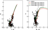 |
Fig. 7 CMDs for the BH118 cluster studied in both NIR and optical Gaia bands. These CMDs were fitted with PARSEC isochrones to infer the age and [Fe/H] for each cluster. |
7 Conclusions
We have provided updated measurements for nine OCs and, for the first time, a detailed characterization of the cluster Juchert 12. Our derived parameters, where available, agree with those provided by Cantat-Gaudin et al. (2020). However, our results conflict with those provided by Kharchenko et al. (2013) and Dias et al. (2014). The CMDs, ages, metallicities, structural parameters, and sky distribution of the clusters indicate that these objects are genuine young, intermediate, or old OCs within the Milky Way disk.
Our derived cluster parameters are presented in Table 4 and compared to the literature values. We derived the cluster reddening, extinction, distance, vertical component, and tangential velocity. Our derived extinctions (AKs) range from 0.07 ± 0.03 to 0.57 ± 0.04, colour excess (E(J - Ks)) from 0.16 ± 0.03 to 0.60 ± 0.03, distances (D) from 2.19 ± 0.06 kpc to 8.94 ± 0.06 kpc, and Galactocentric distances (RG) from 7.82 to 15.08 kpc. The Z component ranges from −0.09 to 0.34 kpc, and tangential velocities (VT) from 30.59 to 245.42 km/s.
We also computed the age and metallicity by fitting PARSEC isochrones, finding ages (t) from 20 Myr to 5 Gyr and metallicity ([Fe/H]) from −0.5 to 0.5 dex. Structural parameters were derived, with core radii (rc) ranging from 0.71 to 5.21′, tidal radii (rt) from 3.6′ to 12.0′, and concentration indices (c) from 0.36 to 0.83. These measurements confirm that the nine clusters examined are genuine young, intermediate, or old OCs. Spectroscopic follow-up is necessary to constrain the metallicity and chemical abundances of the clusters. Additionally, spectroscopic data will help determine the orbital parameters of each cluster.
Acknowledgements
We gratefully acknowledge the use of data from the ESO Public Survey program IDs 179.B-2002 and 198.B-2004 taken with the VISTA telescope and data products from the Cambridge Astronomical Survey Unit. This work has made use of data from the European Space Agency (ESA) mission Gaia (https://www.cosmos.esa.int/gaia), processed by the Gaia Data Processing and Analysis Consortium (DPAC, https://www.cosmos.esa.int/web/gaia/dpac/consortium). Funding for the DPAC has been provided by national institutions, in particular, the institutions participating in the Gaia Multilateral Agreement. This publication makes use of data products from the Two Micron All Sky Survey, which is a joint project of the University of Massachusetts and the Infrared Processing and Analysis Center/California Institute of Technology, funded by the National Aeronautics and Space Administration and the National Science Foundation. We would also like to thank the reviewer for the constructive feedback, which has improved the quality of our manuscript and strengthened our discussion. C.O. Obasi gratefully acknowledges the grants support provided by the Joint Committee ESO-Government of Chile under the agreement 2023 ORP 062/2023. J.G.F.-T. gratefully acknowledges the grants support provided by ANID Fondecyt Iniciación No. 11220340, ANID Fondecyt Postdoc No. 3230001 (Sponsoring researcher) from the Joint Committee ESO-Government of Chile under the agreement 2021 ORP 023/2021 and 2023 ORP 062/2023. D.M. gratefully acknowledges support from the Center for Astrophysics and Associated Technologies CATA by the ANID BASAL projects ACE210002 and FB210003, by Fondecyt Project No. 1220724. M.G. gratefully acknowledges support from Fondecyt through grant 1240755.
Appendix A Additional figures
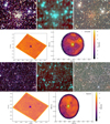 |
Fig. A.1 Same as Fig. 2 but for the clusters Schuster and Saurer 3. |
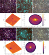 |
Fig. A.2 Same as Fig. 2 but for the clusters FSR 1521 and Saurer 2. |
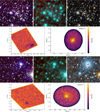 |
Fig. A.3 Same as Fig. 2 but for the clusters Haffner 10 and Juchert 12. The right-hand image in the first and third panels is from Pan-STARRS instead of DECaPS. |
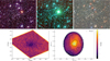 |
Fig. A.4 Same as Fig. 2 but for the cluster Pismis3. |
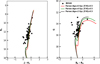 |
Fig. A.5 CMDs of the BH144 cluster studied in both NIR and optical Gaia bands. These CMDs were fitted with PARSEC isochrones to infer the age and [Fe/H] for each cluster. |
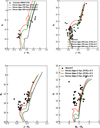 |
Fig. A.6 Same as Fig. 11 but for Schuster (upper left), Saurer 2 (upper right), and Saurer 3 (bottom panel). CMDs are not presented for clusters with high optical extinctions, AG >4. |
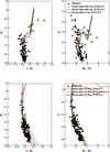 |
Fig. A.7 Same as Fig. 11 but for FSR1521 and Haffner10. For FSR1521, despite the extinction value AV>4, the Gaia CMD is well populated in the main sequence, distinguishing it from other CMDs with similar extinction values. Consequently, we calculated the distance modulus using the distance measured from the parallax. |
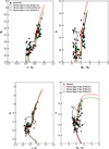 |
Fig. A.8 Same as Fig. 11 but for Juchert12 and Pismis3. |
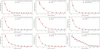 |
Fig. A.9 RDP of the clusters. Black points represent the number of stars per unit area within an annular bin. The red line indicates the best-fit King model profile (King 1962). |
References
- Abuter, R., Amorim, A., Bauböck, M., et al. 2019, A&A, 625, L10 [NASA ADS] [CrossRef] [EDP Sciences] [Google Scholar]
- Alonso-García, J., Minniti, D., Catelan, M., et al. 2017, ApJ, 849, L13 [Google Scholar]
- Alonso-García, J., Saito, R. K., Hempel, M., et al. 2018, A&A, 619, A4 [Google Scholar]
- Alves, D. R., Rejkuba, M., Minniti, D., & Cook, K. H. 2002, ApJ, 573, L51 [NASA ADS] [Google Scholar]
- Angelo, M., Santos, J., Corradi, W., & Maia, F. 2019, A&A, 624, A8 [Google Scholar]
- Ashman, K. M., Bird, C. M., & Zepf, S. E. 1994, AJ, 108, 2348 [Google Scholar]
- Babusiaux, C., Van Leeuwen, F., Barstow, M. A., et al. 2018, A&A, 616, A10 [NASA ADS] [CrossRef] [EDP Sciences] [Google Scholar]
- Bressan, A., Marigo, P., Girardi, L., et al. 2012, MNRAS, 427, 127 [NASA ADS] [CrossRef] [Google Scholar]
- Buckner, A. S., & Froebrich, D. 2013, MNRAS, 436, 1465 [NASA ADS] [CrossRef] [Google Scholar]
- Cantat-Gaudin, T., Krone-Martins, A., Sedaghat, N., et al. 2019, A&A, 624, A126 [NASA ADS] [CrossRef] [EDP Sciences] [Google Scholar]
- Cantat-Gaudin, T., Anders, F., Castro-Ginard, A., et al. 2020, A&A, 640, A1 [NASA ADS] [CrossRef] [EDP Sciences] [Google Scholar]
- Cardelli, J. A., Clayton, G. C., & Mathis, J. S. 1989, AJ, 345, 245 [NASA ADS] [Google Scholar]
- Carraro, G., & Chiosi, C. 1994, A&A, 287, 761 [NASA ADS] [Google Scholar]
- Castro-Ginard, A., Jordi, C., Luri, X., et al. 2018, A&A, 618, A59 [NASA ADS] [CrossRef] [EDP Sciences] [Google Scholar]
- Castro-Ginard, A., Jordi, C., Luri, X., et al. 2022, A&A, 661, A118 [NASA ADS] [CrossRef] [EDP Sciences] [Google Scholar]
- Dias, W., Monteiro, H., Caetano, T., et al. 2014, A&A, 564, A79 [NASA ADS] [CrossRef] [EDP Sciences] [Google Scholar]
- Emerson, J., & Sutherland, W. 2010, The Messenger, 139, 2 [NASA ADS] [Google Scholar]
- Friel, E. 1995, ARA&A, 33, 381 [NASA ADS] [Google Scholar]
- Friel, E. D., Jacobson, H. R., & Pilachowski, C. A. 2010, AJ, 139, 1942 [NASA ADS] [CrossRef] [Google Scholar]
- Frinchaboy, P. M., Majewski, S. R., Crane, J. D., et al. 2004, ApJ, 602, L21 [Google Scholar]
- Gaia Collaboration (Brown, A. G. A., et al.) 2016, A&A, 595, A2 [NASA ADS] [CrossRef] [EDP Sciences] [Google Scholar]
- Gaia Collaboration (Vallenari, A., et al.) 2021, A&A, 649, A1 [NASA ADS] [CrossRef] [EDP Sciences] [Google Scholar]
- Garro, E., Minniti, D., Alessi, B., et al. 2022a, A&A, 659, A155 [NASA ADS] [CrossRef] [EDP Sciences] [Google Scholar]
- Garro, E., Minniti, D., Gómez, M., et al. 2022b, A&A, 662, A95 [NASA ADS] [CrossRef] [EDP Sciences] [Google Scholar]
- Garro, E., Minniti, D., Alonso-García, J., et al. 2024, A&A, 688, L3 [NASA ADS] [CrossRef] [EDP Sciences] [Google Scholar]
- González-Fernández, C., Hodgkin, S. T., Irwin, M. J., et al. 2018, MNRAS, 474, 5459 [Google Scholar]
- Hao, C., Xu, Y., Wu, Z., et al. 2022, A&A, 660, A4 [NASA ADS] [CrossRef] [EDP Sciences] [Google Scholar]
- Kharchenko, N., Piskunov, A., Schilbach, E., Röser, S., & Scholz, R.-D. 2013, A&A, 558, A53 [NASA ADS] [CrossRef] [EDP Sciences] [Google Scholar]
- King, I. 1962, AJ, 67, 471 [Google Scholar]
- Kronberger, M., Teutsch, P., Alessi, B., et al. 2006, A&A, 447, 921 [NASA ADS] [CrossRef] [EDP Sciences] [Google Scholar]
- Marigo, P., Girardi, L., Bressan, A., et al. 2017, ApJ, 835, 77 [Google Scholar]
- Minniti, D., Lucas, P., Emerson, J., et al. 2010, New Astron., 15, 433 [NASA ADS] [CrossRef] [Google Scholar]
- Montgomery, K. A., Janes, K. A., & Phelps, R. L. 1994, AJ, 108, 585 [NASA ADS] [Google Scholar]
- Muratov, A. L., & Gnedin, O. Y. 2010, AJ, 718, 1266 [NASA ADS] [Google Scholar]
- Nataf, D. M., Gonzalez, O. A., Casagrande, L., et al. 2015, MNRAS, 456, 2692 [Google Scholar]
- Nishiyama, S., Tamura, M., Hatano, H., et al. 2009, ApJ, 696, 1407 [NASA ADS] [CrossRef] [Google Scholar]
- Obasi, C., Gomez, M., Minniti, D., & Alonso-Garcia, J. 2021, A&A, 654, A39 [NASA ADS] [CrossRef] [EDP Sciences] [Google Scholar]
- Obasi, C., Gomez, M., Minniti, D., et al. 2023, A&A, 670, A18 [NASA ADS] [CrossRef] [EDP Sciences] [Google Scholar]
- Obasi, C., Gómez, M., Minniti, D., et al. 2024, MNRAS, 529, 3075 [NASA ADS] [CrossRef] [Google Scholar]
- Phelps, R. 1994, AJ, 107, 1079 [NASA ADS] [CrossRef] [Google Scholar]
- Ruiz-Dern, L., Babusiaux, C., Arenou, F., Turon, C., & Lallement, R. 2018, A&A, 609, A116 [NASA ADS] [CrossRef] [EDP Sciences] [Google Scholar]
- Saito, R. K., Hempel, M., Minniti, D., et al. 2012, A&A, 537, A107 [NASA ADS] [CrossRef] [EDP Sciences] [Google Scholar]
- Saito, R., Hempel, M., Alonso-García, J., et al. 2024, A&A, 689, A148 [NASA ADS] [CrossRef] [EDP Sciences] [Google Scholar]
- Sanders, W. 1971, A&A, 14, 226 [Google Scholar]
- Saroon, S., Dias, B., Minniti, D., et al. 2024, A&A, 689, A115 [NASA ADS] [CrossRef] [EDP Sciences] [Google Scholar]
- Schlafly, E. F., & Finkbeiner, D. P. 2011, AJ, 737, 103 [NASA ADS] [CrossRef] [Google Scholar]
- Schlegel, D. J., Finkbeiner, D. P., & Davis, M. 1998, ApJ, 500, 525 [Google Scholar]
- Siegert, T. 2019, A&A, 632, L1 [NASA ADS] [CrossRef] [EDP Sciences] [Google Scholar]
- Skrutskie, M., Cutri, R., Stiening, R., et al. 2006, AJ, 131, 1163 [Google Scholar]
- Stetson, P. B. 1980, AJ, 85, 387 [NASA ADS] [Google Scholar]
- Tarricq, Y., Soubiran, C., Casamiquela, L., et al. 2022, A&A, 659, A59 [NASA ADS] [CrossRef] [EDP Sciences] [Google Scholar]
- Taylor, M. B. 2005, in Astronomical Data Analysis Software and Systems XIV, 347, 29 [NASA ADS] [Google Scholar]
- Tosi, M., Pulone, L., Marconi, G., & Bragaglia, A. 1998, MNRAS, 299, 834 [Google Scholar]
- Tosi, M., Bragaglia, A., & Cignoni, M. 2007, MNRAS, 378, 730 [Google Scholar]
- Vasilevskis, S., Klemola, A., & Preston, G. 1958, AJ, 63, 387 [NASA ADS] [CrossRef] [Google Scholar]
- York, D. G., Adelman, J., Anderson Jr, J. E., et al. 2000, AJ, 120, 1579 [NASA ADS] [CrossRef] [Google Scholar]
- Zhao, J., & He, Y. 1990, A&A, 237, 54 [Google Scholar]
- Zhao, J., & Shao, Z. 1994, A&A, 288, 89 [Google Scholar]
All Tables
Cluster name, coordinates (RA and Dec), Galactic coordinates (l and b), VVVX tile corresponding to each cluster, and literature references.
Derived physical parameters for each cluster compared with literature values from Cantat-Gaudin et al. (2020), Kharchenko et al. (2013), and Dias et al. (2014).
All Figures
|
Fig. 1 VVVX density maps and Gaussian KDEs for the clusters FSR 1333 (upper panels) and FSR 1651 (lower panels). |
| In the text | |
|
Fig. 2 Top panel: multi-band images of the OC BH118 from 2MASS (left), WISE (middle), and DECaPS (right). Second panel: cluster density map highlighting the darkest region as the cluster location (left) and the KDE distribution (right). Third and fourth panels: same but for BH144. |
| In the text | |
|
Fig. 3 Histograms of PMs (μα* and μδ), highlighting the distributions of the cluster (blue) and field (grey) populations along with their respective mean values. |
| In the text | |
|
Fig. 4 Membership probability as a function of Ks magnitude. The dashed horizontal line indicates the 90% cluster membership threshold for BH144. |
| In the text | |
|
Fig. 5 Upper panel: 2MASS NIR CMD (Ks vs J-Ks). On the right, the RC overdensity is visible on the density map, and the horizontal line indicates the density peak. Lower panel: same but with optical Gaia data (G vs BP-RP) for Pismis3. |
| In the text | |
|
Fig. 6 Sky distribution plot of all nine clusters, showing their positions in Galactic coordinates (longitude l and latitude b), with colour representing their tangential velocities. |
| In the text | |
|
Fig. 7 CMDs for the BH118 cluster studied in both NIR and optical Gaia bands. These CMDs were fitted with PARSEC isochrones to infer the age and [Fe/H] for each cluster. |
| In the text | |
|
Fig. A.1 Same as Fig. 2 but for the clusters Schuster and Saurer 3. |
| In the text | |
|
Fig. A.2 Same as Fig. 2 but for the clusters FSR 1521 and Saurer 2. |
| In the text | |
|
Fig. A.3 Same as Fig. 2 but for the clusters Haffner 10 and Juchert 12. The right-hand image in the first and third panels is from Pan-STARRS instead of DECaPS. |
| In the text | |
|
Fig. A.4 Same as Fig. 2 but for the cluster Pismis3. |
| In the text | |
|
Fig. A.5 CMDs of the BH144 cluster studied in both NIR and optical Gaia bands. These CMDs were fitted with PARSEC isochrones to infer the age and [Fe/H] for each cluster. |
| In the text | |
|
Fig. A.6 Same as Fig. 11 but for Schuster (upper left), Saurer 2 (upper right), and Saurer 3 (bottom panel). CMDs are not presented for clusters with high optical extinctions, AG >4. |
| In the text | |
|
Fig. A.7 Same as Fig. 11 but for FSR1521 and Haffner10. For FSR1521, despite the extinction value AV>4, the Gaia CMD is well populated in the main sequence, distinguishing it from other CMDs with similar extinction values. Consequently, we calculated the distance modulus using the distance measured from the parallax. |
| In the text | |
|
Fig. A.8 Same as Fig. 11 but for Juchert12 and Pismis3. |
| In the text | |
|
Fig. A.9 RDP of the clusters. Black points represent the number of stars per unit area within an annular bin. The red line indicates the best-fit King model profile (King 1962). |
| In the text | |
Current usage metrics show cumulative count of Article Views (full-text article views including HTML views, PDF and ePub downloads, according to the available data) and Abstracts Views on Vision4Press platform.
Data correspond to usage on the plateform after 2015. The current usage metrics is available 48-96 hours after online publication and is updated daily on week days.
Initial download of the metrics may take a while.