| Issue |
A&A
Volume 695, March 2025
|
|
|---|---|---|
| Article Number | A272 | |
| Number of page(s) | 6 | |
| Section | Celestial mechanics and astrometry | |
| DOI | https://doi.org/10.1051/0004-6361/202452459 | |
| Published online | 26 March 2025 | |
The Gaia astrometric catalogue and secular aberration drift in proper motions
1
Leiden Observatory, Leiden University,
Einsteinweg 55,
2333
CC Leiden, The Netherlands
2
Astronomisches Rechen-Institut, Zentrum für Astronomie der Universität Heidelberg,
Mönchhofstr. 12–14,
69120
Heidelberg, Germany
3
Lohrmann Observatory, Technische Universität Dresden,
Mommsenstraße 13,
01062
Dresden, Germany
★ Corresponding author; This email address is being protected from spambots. You need JavaScript enabled to view it.
Received:
1
October
2024
Accepted:
27
February
2025
Abstract
Context. A recent paper demonstrated the existence of a secular aberration drift term in stellar proper motions that arises when transforming an astrometric catalogue defined for an observer at rest with respect to the Solar System barycentre to some other reference frame in which, for example, the observer is at rest with respect to the Galactic centre. Such a transformation requires an accurate and precise estimate of the velocity of the Solar System barycentre. It was argued that the Gaia catalogue construction should account for this effect and also for the aberrational effect due to acceleration of the Solar System barycentre.
Aims. We argue that these two effects should not be accounted for in the construction of the Gaia astrometric catalogue.
Methods. We briefly review the Gaia catalogue reference frame, the concepts of stellar aberration and secular aberration drift, and their observable consequences.
Results. The Gaia catalogue is (and should be) constructed in the barycentric celestial reference system: the reference system with the origin at the Solar System barycentre as defined by the underlying Solar System ephemerides. We explain that the Gaia catalogue is consistent with the International Celestial Reference System despite the presence of proper motion terms due to the acceleration of the Solar System barycentre. We also explain why transformation of the astrometry to a frame in which the observer is at rest with respect to the Galactic centre or distant universe is not needed for the interpretation of stellar kinematics, and that there are practical concerns with such a transformation.
Conclusions. Estimations of the velocity and acceleration of the Solar System barycentre, although important as a matter of scientific investigation, are not needed for the construction of the Gaia astrometric catalogue.
Key words: astrometry / proper motions / reference systems
© The Authors 2025
 Open Access article, published by EDP Sciences, under the terms of the Creative Commons Attribution License (https://creativecommons.org/licenses/by/4.0), which permits unrestricted use, distribution, and reproduction in any medium, provided the original work is properly cited.
This article is published in open access under the Subscribe to Open model. This email address is being protected from spambots. You need JavaScript enabled to view it. to support open access publication.
1 Introduction
As a demonstration of the high quality of the astrometry published in Gaia Early Data Release 3 (Gaia Collaboration 2021a, 2016), an accompanying paper (Gaia Collaboration 2021b) presented a measurement of the acceleration of the Solar System barycentre (SSB) with respect to the rest frame of the distant universe, represented by a large number of quasars on the whole sky. The result rests on the fact that the changing space velocity vector, υc, of the SSB relative to the rest frame of the distant universe (i.e. the SSB acceleration  ) leads to a systematic proper motion pattern in quasar-like sources, which is measurable with Gaia. This proper motion pattern reflects the change in the effect of aberration on source positions (due to the changing SSB velocity vector, υc), which is sometimes referred to in the literature as ‘secular aberration drift’.
Recently, Liu et al. (2024) derived the presence of an additional secular aberration drift term caused by the changing effect over time of stellar aberration for nearby sources (i.e. not at cosmological distances), in turn caused by the changing line-of-sight direction to the sources (due to the motion of the sources with respect to the SSB). Liu et al. (2024) considered an observer at the SSB at rest with respect to the extragalactic background but in their work adopted the results from Reid et al. (2019) for the velocity of the SSB, which is actually the velocity with respect to our Galaxy, υg. According to their Eq. (16), the additional secular aberration drift term causes a small change in the proper motion of a source that is proportional to υg and the proper motion itself. They conclude that such a bias should therefore be considered in the reduction of Gaia astrometric data. Specifically, they propose that stellar proper motions should be corrected for the secular aberration drift effects by: (1) removing the term caused by the SSB acceleration; and then (2) removing the additional secular aberration drift term by iteratively determining from the astrometric catalogue the velocity υg of the SSB and the corrections to the catalogue proper motions. The aim would be to make the (Gaia) stellar reference frame consistent with the ‘extragalactic reference frame’ (by which Liu et al. 2024 mean the rest frame of our Galaxy), and to improve our understanding of stellar kinematics via the removal of apparent proper motion components.
We note that the two velocities, υg and υc , differ in terms of both their directions and absolute values. The υc is the velocity of the SSB relative to the distant universe. In the standard cosmological model, υc can be measured, for example, from the dipole of the cosmic microwave background radiation and was recently estimated as |υc| ≈ 370 km s−1 (Planck Collaboration III 2020). On the other hand, υg is the velocity of the SSB with respect to the rest frame of the Galaxy. It can be measured from the kinematics of the stars of our Galaxy and/or from accurate astrometric measurements of the radio source Sgr A*; it has been found to be |υg| ≈ 248 km s−1 (Reid & Brunthaler 2020).
In this paper we explain why the corrections proposed by Liu et al. (2024) are, as a matter of principle, not pursued in the construction of the Gaia catalogue, including for the upcoming data releases 4 and 5. Although the discussion in the following sections is framed in terms of Gaia astrometry, we stress that this paper and its conclusions apply to any modern astrometric data defined within the International Celestial Reference System (ICRS).
2 The Gaia catalogue reference frame
The astrometric data in the Gaia data releases are referred to the barycentric celestial reference system (BCRS; Soffel et al. 2003). The origin of the BCRS coincides with the SSB as defined by the underlying Solar System ephemerides. The spatial axes of the BCRS are aligned with the ICRS (Arias et al. 1995; Feissel & Mignard 1998). This choice of reference system means that Gaia source positions and proper motions are those seen by an observer at rest at the origin of the BCRS and co-moving with that origin. We discuss the consistency of the Gaia catalogue with the ICRS in Sect. 4.
3 Aberration, secular aberration drift, and observable consequences
In this section we provide an alternative derivation of the Liu et al. (2024) result and clarify under what circumstances the effects of aberration on source positions and proper motions can be observed. The definition of stellar aberration in the Explanatory Supplement to the Astronomical Almanac (Urban & Seidelmann 2013) is as follows: ‘The relativistic apparent angular displacement of the observed position of a celestial object from its geometric position, caused by the motion of the observer in the reference system in which the trajectories of the observed object and the observer are described1.’ This definition grasps the main point of aberration: the aberrational correction should be applied in order to work directly with the (time-dependent) geometric positions of observed sources relative to a given observer as defined in the selected reference system. The geometric positions both in the Newtonian and relativistic contexts are defined in some selected reference system A with spatial coordinates x = xi, i = 1,2,3. In those coordinates the trajectory of a source is xsrc(t) while that of the observer is xobs (t). Here t is the coordinate time of the selected reference system (reducing to the Newtonian absolute time in the Newtonian approximation). Then the geometric position of the source is the unit vector u(tobs) = 〈xsrc(tem) − xobs(tobs)〉, where tobs is the time of observation, tem is the time of emission of the signal that reaches the observer at time tobs, and 〈…〉 denotes the normalisation to a unit vector.
The standard parameterisation of u(tobs) gives the standard astrometric parameters of a source: positions, proper motions, and parallaxes at a certain epoch. Detailed discussions of various aspects of the parameterisation can be found in Lindegren et al. (2012), Butkevich & Lindegren (2014), and Klioner (2003). Along with the trajectories of the observer and the source, the astrometric parameters are also defined in the reference system A with time t and spatial coordinates x. The standard parameterisation of u(tobs), which is intended for single stars, assumes that the spatial trajectory of xsrc(t) is a linear function of time. This approximation should be sufficiently correct at least during the time interval covered by astrometric data, but is usually considered true during the reasonable interval of time of a few centuries discussed by modern astrometry. The requirement that xsrc(t) should be sufficiently close to a linear function of time gives certain constraints that determine which reference systems can be used in astrometry at a given level of accuracy and which cannot. In particular, to avoid rotation of the spatial coordinates the suitable reference systems should be pseudo-inertial in the Newtonian approximation or its relativistic generalisations. In addition the motion of the origin of the reference system should be suitable. For example, a reference system with the origin at the centre of mass of the Earth with its quasi-periodic motion in the Solar System with a period of about 1 year is not adequate for astrometry as soon as the observational accuracy exceeds several arcseconds. On the other hand, a reference system with the origin at the SSB, as defined by a modern Solar System ephemeris, can be used in astrometry at the microarcsecond level: the non-linearity of stellar trajectories relative to the SSB due to the Galactic gravitational forces is beyond reach even for Gaia astrometry (ESA 2000, Sect. 1.10, p. 102). From hereon, the origin of A will be fixed at the SSB and its spatial coordinates will be denoted as xA . This is the reference system, in which the Gaia catalogue is constructed.
3.1 Aberration and secular aberration drift
Following Liu et al. (2024), we considered another reference system, ℬ, with spatial coordinates xℬ2. At some moment of time, the origin of ℬ moves with respect to that of A with a velocity V that is not necessarily a constant. Reciprocally, the velocity of the origin of A relative to ℬ at the same moment of time is -V. We assumed here that reference system ℬ can also be used in astrometry at the same level of accuracy as A. In particular, this is true if V is sufficiently close to a constant. The spatial coordinates of the reference systems A and ℬ are related to each other by a generalised Lorentz transformation (Soffel et al. 2003). For our discussion, the Newtonian limit is sufficient:
 (1)
(1)
where rAℬ (t) is the position of the origin of ℬ in A at the moment t, so that  . Equation (1) can be used to relate the trajectories of the sources and the observer in the reference systems A and ℬ. The transformation of the trajectories also allows one to transform the standard astrometric parameters of the sources. This means that the astrometric parameters obtained in A can be transformed to those measured in ℬ and vice versa without loss of information, provided V is known accurately and to a precision that is compatible with the astrometric measurement precision. This point is important for the discussion in Sect. 4.
On the other hand, transformation (1) also gives the expression for the aberration of light when one considers the light ray trajectory passing through the observer at the moment of observation from the apparent direction u(tobs): xlight(t) = xobs(tobs) − c u(tobs) (t − tobs) + O(c−1). Applying Eq. (1) to the light ray directions (and placing the observers in A and ℬ at the same physical location in space) allows one to relate the directions uℬ and uA , and using the normalisation u · u = 1 one gets3
 (2)
(2)
The situation is shown schematically in Fig. 1, in which uA and uℬ are the unit vectors representing the geometric directions for the same observation in reference systems A and ℬ, respectively. In particular, for ℬ, we can choose the reference system moving relative to A with velocities −υc or −υg, as discussed in Sect. 1. Thus, ℬ can be at rest either relative to the Galactic centre or relative to the distant universe. Below we sometimes speak of observers A and ℬ, whose positions coincide with the origins of the respective reference systems at any moment of time.
The aberration effect in Eq. (2) can change over time:
 (3)
(3)
with dV/ dt = a and where uA is assumed not to change. This is referred to as ‘secular aberration drift’ and is what Gaia Collaboration (2021b) used to estimate a for the SSB. What Liu et al. (2024) pointed out is that the source direction uA also changes over time so that the more complete equation for the change in δu reads
![Mathematical equation: ${{{\rm{d}}\delta {\bf{u}}} \over {{\rm{d}}t}} = {\bf{a}} - {{{{\bf{u}}_{\cal A}} \cdot {\bf{a}}} \over c}{{\bf{u}}_{\cal A}} - {1 \over c}\left[ {\left( {{{{\rm{d}}{{\bf{u}}_{\cal A}}} \over {{\rm{d}}t}} \cdot {\bf{V}}} \right){{\bf{u}}_{\cal A}} + \left( {{{\bf{u}}_{\cal A}} \cdot {\bf{V}}} \right){{{\rm{d}}{{\bf{u}}_{\cal A}}} \over {{\rm{d}}t}}} \right].$](/articles/aa/full_html/2025/03/aa52459-24/aa52459-24-eq6.png) (4)
(4)
This shows that changes in the lines of sight to sources (due to the change in geometric direction as observed in reference system A) can cause an additional secular aberration drift term. We now write the change of uA as a function of time in terms of the normal triad [p0, q0, r0] (see Sect. 3.2 of Lindegren et al. 2012) at the reference epoch t = tep (where uA(tep) = r0) and the proper motion µ0 at tep:

with µα*,0 and µδ,0 the proper motions in right ascension and declination at tep . Here we assumed that the observer is situated at the origin of A and omitted the parallax effect (which is not of interest here) and the effect of the radial proper motion, µr, which does not lead to a change in uA (see Lindegren et al. 2012, their Eq. (4)). Working out the additional term gives us the total secular aberration drift:
![Mathematical equation: ${{{\rm{d}}\delta {\bf{u}}} \over {{\rm{d}}t}} = {{\bf{a}} \over c} - {{{{\bf{r}}_0} \cdot {\bf{a}}} \over c}{{\bf{r}}_0} - {1 \over c}\left[ {\left( {{{\bf{\mu }}_0} \cdot {\bf{V}}} \right){{\bf{r}}_0} + \left( {{{\bf{r}}_0} \cdot {\bf{V}}} \right){{\bf{\mu }}_0}} \right].$](/articles/aa/full_html/2025/03/aa52459-24/aa52459-24-eq8.png) (5)
(5)
Using the fact that the term (µ0 · V) r0 does not lead to a transverse proper motion, the result is that the additional term in the secular aberration drift for stellar proper motions is
 (6)
(6)
This is the Liu et al. (2024) result that they derived by considering the effect of the epoch propagation of source positions on the aberration in Eq. (2) and then making an approximation for small epoch differences. Hence, the full secular aberration drift in proper motion is
 (7)
(7)
This equation shows the changes in the apparent proper motion components between the reference systems of observers A and ℬ due to the changes in V and uA . We stress that the secular aberration drift terms simply result from the transformation between reference systems A and ℬ and thus strictly describe the differences between the proper motions of the same sources observed in A or ℬ. The differences are specific to the relative motion of observers A and ℬ described by V and a.
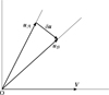 |
Fig. 1 Schematic illustration of stellar aberration. The observer at O is moving with velocity V with respect to reference system A and observes the object in the direction uℬ . The geometric direction of the object in reference system A is uA. Based on Fig. 7.3 in the Explanatory Supplement to the Astronomical Almanac (Urban & Seidelmann 2013). |
3.2 When are aberration effects observable in practice?
We next asked whether aberration effects can be observed from reference system A. This question arises because Liu et al. (2024) consider the case where the astrometric source parameters as established in A are to be transformed to a reference system ℬ in which the secular aberration drift terms are removed, enabling a better study of, for example, galactic dynamics. This requires that the aberration effects are established by the observer in A based on observations made in that same reference system A. We first stress an important point again: the source positions reported by an observer at rest in reference system A are geometric in that reference system. Stellar aberration effects that were not removed in the astrometric data processing, can only be observed if a certain pattern in the geometric source positions uA in A can be related unambiguously to the effects of aberration.
We first considered the static aberration effect described by Eq. (2) assuming V and uA are unchanging. In this case the observer ℬ is moving at constant velocity V and the stellar aberration leads to a static change in source directions uℬ compared to the directions uA . The source positions as seen by observer B will be distorted with respect to the positions in A such that sources will tend to concentrate towards the direction of motion V (see fig:schematic). Conversely, the source positions as seen by observer A will be distorted with respect to the positions in ℬ such that the sources will tend to concentrate towards the direction −V. However this distortion can only be measured by observer A if they know the source directions in ℬ (which is an academic case only), or if the source directions can be assumed to be uniform over the sky in a specific reference system. For distant quasi-stellar objects (QSOs), the assumption of a uniform sky distribution in the rest frame of the distant universe is reasonable (and is used in the literature to constrain the cosmic velocity uc of the Solar System; see e.g. Ellis & Baldwin 1984, and references to that work). However, for stars this is far from true due to their highly non-uniform and imperfectly known spatial distribution in the Milky Way. Hence, the static aberration effect is not observable in practice and is normally ignored for stars.
A well-known observable aberration effect is that of the annual stellar aberration. Here the observer is orbiting the SSB, so their velocity is constantly changing direction, which causes a changing aberration effect for all stars. The resulting apparent annual motion on the sky, with amplitude ∼20 arcsec, is the same for all stars (not dependent on their distance). The most simple explanation for this pattern is the effect of aberration, which can be calculated precisely by transforming the directions seen by the observer in orbit around the SSB to the directions seen by an observer at rest at the SSB. Indeed, in the Gaia astrometric data processing source positions are referred to the SSB and corrections for the annual stellar aberration are applied. In this case the motion of Gaia with respect to the SSB is very accurately known so the annual aberration effects can be taken out to sufficient accuracy.
Next we turned to Eq. (7) and asked whether there are geometric proper motion patterns observable in A that can most easily be explained as being due to aberration. QSO-like sources are sufficiently distant that we can safely assume that their proper motions are zero, which means that for these sources the acceleration-related terms in Eq. (7) lead to a global proper motion pattern on the sky that can be exploited to estimate ac , as done in Gaia Collaboration (2021b). The observability of the acceleration-related secular aberration drift thus relies on our access to a sample of very distant sources which have zero geometric proper motions in the rest frame of the distant universe (or any other reference system moving relative to that rest frame with a constant velocity). It is discussed in great detail in Gaia Collaboration (2021b) why no reasonable estimate of ac can be achieved using stars in our Galaxy: the proper motions of stars are not predictable to the relevant level of accuracy.
Quasi-stellar-object-like sources are of no use in observing the additional secular aberration drift term from Eq. (6) because for these objects µ0 is zero. What sample of sources might allow this drift term to be observed? Here we have to rely on nearby sources with significant proper motions in order to get a non-zero ∆µ. Figure 1 in Liu et al. (2024) illustrates that the factor r0 ⋅ V shows a global pattern on the sky. Possibly this pattern could be revealed if a sample of sources would be available for which we can on physical grounds assume that these exhibit an ordered proper motion field µ0 (α, δ) in A or any other well-defined reference system, which would be modulated in a detectable way by r0 · V. Such a sample does not exist, as stars in the Milky Way exhibit a complex proper motion field, varying in direction and amplitude, which completely hides the effect sought after. Hence, the additional secular aberration drift term in stellar proper motions is in practice not observable in A.
Moreover, as mentioned above the additional secular aberration drift term describes the difference between the proper motions as observed in A and ℬ. Not applying this additional aberrational effect does not alter the residuals of the astrometric solution. One can always recompute one set of proper motions into another as soon as both reference systems are strictly defined.
4 Should the Gaia catalogue be corrected for secular aberration drift?
Despite the effect described in Liu et al. (2024) not being observable, one could still argue that we know that the SSB moves and that with an estimate of V and ac one could transform the stellar proper motions to a reference system in which the observer is at rest with respect to the Galactic centre or distant universe. Liu et al. (2024) propose that the Gaia astrometry be corrected for the effects of secular aberration drift on the proper motions (1) to make sure the stellar reference frame aligns with the extragalactic reference frame; and (2) to advance our understanding of stellar kinematics.
4.1 The reference frame and secular aberration drift
Concerning the first point above, the extragalactic reference frame is not well defined in Liu et al. (2024). For the truly extragalactic reference frame, the rest frame of the distant universe and thus V = −υc should be used. Instead, Liu et al. (2024) consider V = −υg and the rest frame of our Galaxy which is better referred to as the ‘galactic reference frame’. Moreover, we note that the reference system suggested by Liu et al. (2024) is not defined in a self-consistent way: the authors suggest to correct for the effects of υg in proper motions, but ignore those effects in positions; thus the standard parametrisation of uℬ(tobs) no longer works. In addition the corrections for the effects of acceleration ac and υℬ are inconsistent, as ac corresponds to υc and not υg .
We emphasise that the Gaia catalogue (and thus the stellar reference frame) is constructed to be consistent with the ICRS by aligning the Gaia catalogue positions with the International Celestial Reference Frame (ICRF, specifically its thrid realisation ICRF3), in the case of Gaia DR3 using ICRF3 sources present in the Gaia catalogue. In this process, the coordinates of the ICRF3 sources are propagated to the epoch of the Gaia catalogue as prescribed by the ICRF3 (Charlot et al. 2020). To ensure that the Gaia celestial reference frame is globally nonrotating with respect to the distant universe, the rotational state of the Gaia catalogue was chosen such that a large number of QSOs (not only the ICRF3 sources) show no common rotation in their proper motions (see Gaia Collaboration 2022). We note here that the additional proper motions due to the acceleration of the SSB are mathematically orthogonal to the frame rotation and do not influence it (see Mignard & Klioner 2012). The proper motions of stars are not at all used to define the reference frame for Gaia.
The ICRS definition (Arias et al. 1995) specifies the orientation of the axes to be fixed. Those axes can be materialised both by celestial sources with constant positions and by sources with time-dependent positions. The only necessary condition is that the positions of these sources are known at any moment of time in the ICRS axes. Naturally, sources with no proper motion are more convenient for the materialisation and until 2018 the ICRF realisations assumed the positions of quasars as constant. With ICRF3 (Charlot et al. 2020) the accuracy of very long-baseline interferometry (VLBI) astrometry has reached the level where systematic proper motions due to the SSB acceleration should be taken into account (see Charlot et al. 2020, Sect. 3.2 and references therein for a discussion and brief history of this topic). Hence, the choice made in the construction of the ICRF3 to include a defining acceleration of the SSB in the data analysis (with an amplitude inferred from the VLBI data) in order to account for the systematic proper motions. This allows one to derive ICRF3 source positions consistent with the ICRS axes and correctly propagate the ICRF3 source positions to any desired epoch (Charlot et al. 2020). Unlike the VLBI astrometry, in the Gaia data processing quasars are treated as normal astrometric sources and their measured proper motions are published. Those proper motions contain both the systematic proper motions due to the SSB acceleration and the individual apparent proper motions of these sources. The published proper motions allow one to compute the positions of the Gaia quasars for any moment of time in the ICRS axes so that the orientation of the Gaia reference frame is fully compatible with the ICRS. On the other hand, the proper motions published by Gaia can be used by the community to measure the SSB acceleration, potentially improving the results.
What about the reference frame and the additional secular aberration drift term in stellar proper motions? As stressed above, the positions and proper motions as listed in the Gaia catalogue reflect the geometric directions and their change over time as seen by observer A and thus form an accurate observational description of the celestial sphere. An important role of the Gaia catalogue is in predicting future and past positions of sources on the sky in reference system A (epoch propagation) for applications such as stellar occultations, astrometric data reduction of surveys anchored to Gaia, catalogue matching, and telescope pointing. If the Gaia catalogue were to list astrometric parameters as seen by observer ℬ (i.e. removing the secular aberration drift terms), the use of this astrometry by observer A would actually lead to erroneous predictions of future or past positions of sources, as observed in reference system A, and thus spoil the above mentioned applications (unless one introduces a more complex algorithm that first undoes the transformation from A to ℬ, but this would be very error-prone in practice).
4.2 Secular aberration drift and stellar kinematics
The second point raised by Liu et al. (2024) concerns the desire to study the kinematics of stars and the dynamics of the Milky Way using proper motions free from aberration effects, namely, the ‘true’ proper motions as seen by the observer B with V = −υg . However, according to the relativity principle, observer ℬ is no more fundamental than observer A, meaning that even if different observers moving at constant velocity relative to each other report different stellar kinematics, the dynamics the observers infer should be the same. This is easily seen in the Newtonian limit where the transformation between frames A and ℬ amounts to a velocity offset only, which clearly will not affect the dynamics of any stellar system under study (and we stress that the dynamics will also be the same if Lorentz transformations are involved). Hence, corrections for the term in Eq. (6) are not needed. The term due to the SSB acceleration is sufficiently small at the current precision levels that it can be ignored. Also, its size is far below many Galactic kinematic structures, as detailed in Gaia Collaboration (2021b), and can thus be ignored entirely.
We now discuss a more practical concern. The correction procedure proposed by Liu et al. (2024) depends on an accurate knowledge of the SSB velocity (and acceleration). The velocity has to be estimated from the Gaia data to sufficient accuracy to preserve the accuracy of the measured proper motions. The best relative proper motion uncertainties in the Gaia DR3 catalogue are of order 2.7 × 10⁻⁶ and are expected to improve by a factor of ∼8 in the Gaia DR5. This implies a knowledge of υg at a level considerably better than 100m s−1, while modern estimates (based also on Gaia data) are precise to the few km s−1 level, and are plagued by systematic uncertainties due to stellar kinematics that deviate from a simple rotation curve (see e.g. Almannaei et al. 2024). Moreover, if proper motion corrections at the level of υg/c ~ 8 × 10⁻⁴ are considered important, then presumably corrections at the same level to the other phase space coordinates (stellar positions) are also important. Correcting the celestial positions for aberration subject to preserving the Gaia catalogue relative position uncertainties (of order 5 × 10⁻⁹ for faint stars to 5 × 10⁻¹² for bright stars) would require knowledge of V down to the mm s−1 level4.
A second more fundamental practical concern is the following. Constructing the astrometric catalogue as seen in ℬ by an observer at the SSB at rest with respect to our Galaxy (and thus moving with V = −υg with respect to A) necessitates introducing a priori our uncertain knowledge on the Milky Way galaxy, through υg, ac, and the assumption that  , into an observational catalogue that we would then use to study that same galaxy. This approach would spoil the purely observational result represented by the Gaia catalogue, which is constructed within the very precisely defined BCRS and ICRS and lists well- defined astrometric parameters derived from the measurements using the simplest assumption that stars follow straight line trajectories at constant speed. We advocate that the estimation of υc and υg , as well as their derivatives and possible transformations of the astrometry to a different reference frame, belong to the realm of scientific investigation and that therefore the Gaia catalogue should always be presented as a well-defined and accurate observational result, free from assumptions about the Milky Way galaxy.
5 Conclusion
We have shown that the work presented in Liu et al. (2024), even though the results are correct in the context of considering what an observer at the SSB would see if at rest with respect to the Galactic centre, is of no practical consequence for the construction and publication of the Gaia catalogue. Estimations of the velocity and acceleration of the SSB, and possible transformations of the astrometry to a frame in which the observer is at rest with respect to the Galactic centre or distant universe, are subjects of scientific investigation, not Gaia astrometric catalogue construction.
Acknowledgements
The authors thank Jos de Bruijne for triggering the discussion that resulted in this paper, and the referee for a critical report that prompted a thorough rethinking and clarification of the issues to be addressed. This work has made use of data from the European Space Agency (ESA) mission Gaia (https://www.cosmos.esa.int/gaia), processed by the Gaia Data Processing and Analysis Consortium (DPAC, https://www.cosmos.esa.int/web/gaia/dpac/consortium). Funding for the DPAC has been provided by national institutions, in particular the institutions participating in the Gaia Multilateral Agreement. While preparing this work we made use of the following software: Astropy, a community-developed core Python package for Astronomy (Astropy Collaboration 2013, 2018, 2022, https://www.astropy.org), IPython (Pérez & Granger 2007, https://ipython.org/), Jupyter (https://jupyter.org/), Matplotlib (Hunter 2007, https://matplotlib.org), NumPy (Harris et al. 2020, https://numpy.org), TOPCAT (Taylor 2005, https://www.starlink.ac.uk/topcat/), and the TikZ and PGF packages Tantau (2024). This research has made use of the Astrophysics Data System, funded by NASA under Cooperative Agreement 80NSSC21M00561, and the SIMBAD database (SIMBAD; Wenger et al. 2000) operated at the CDS, Strasbourg, France (CDS).
References
- Almannaei, A. S., Kawata, D., Baba, J., et al. 2024, MNRAS, 529, 1035 [NASA ADS] [CrossRef] [Google Scholar]
- Arias, E. F., Charlot, P., Feissel, M., & Lestrade, J. F. 1995, A&A, 303, 604 [NASA ADS] [Google Scholar]
- Astropy Collaboration (Robitaille, T. P., et al.) 2013, A&A, 558, A33 [NASA ADS] [CrossRef] [EDP Sciences] [Google Scholar]
- Astropy Collaboration (Price-Whelan, A. M., et al.) 2018, AJ, 156, 123 [Google Scholar]
- Astropy Collaboration (Price-Whelan, A. M., et al.) 2022, ApJ, 935, 167 [NASA ADS] [CrossRef] [Google Scholar]
- Butkevich, A. G., & Lindegren, L. 2014, A&A, 570, A62 [NASA ADS] [CrossRef] [EDP Sciences] [Google Scholar]
- Charlot, P., Jacobs, C. S., Gordon, D., et al. 2020, A&A, 644, A159 [EDP Sciences] [Google Scholar]
- Ellis, G. F. R., & Baldwin, J. E. 1984, MNRAS, 206, 377 [NASA ADS] [CrossRef] [Google Scholar]
- ESA 2000, GAIA: Composition, formation and evolution of the Galaxy, Technical Report ESA-SCI(2000)4 (ESA), scientific case online at https://www.cosmos.esa.int/documents/29201/297049/report-science.pdf/9d4395c7-79bb-4a05-ac3a-3b51a16e6c70 [Google Scholar]
- Feissel, M., & Mignard, F. 1998, A&A, 331, L33 [Google Scholar]
- Gaia Collaboration (Prusti, T., et al.) 2016, A&A, 595, A1 [NASA ADS] [CrossRef] [EDP Sciences] [Google Scholar]
- Gaia Collaboration (Brown, A. G. A., et al.) 2021a, A&A, 649, A1 [NASA ADS] [CrossRef] [EDP Sciences] [Google Scholar]
- Gaia Collaboration (Klioner, S. A., et al.) 2021b, A&A, 649, A9 [EDP Sciences] [Google Scholar]
- Gaia Collaboration (Klioner, S. A., et al.) 2022, A&A, 667, A148 [NASA ADS] [CrossRef] [EDP Sciences] [Google Scholar]
- Harris, C. R., Millman, K. J., van der Walt, S. J., et al. 2020, Nature, 585, 357 [NASA ADS] [CrossRef] [Google Scholar]
- Hunter, J. D. 2007, Comput. Sci. Eng., 9, 90 [NASA ADS] [CrossRef] [Google Scholar]
- Klioner, S. A. 2003, AJ, 125, 1580 [Google Scholar]
- Lindegren, L., Lammers, U., Hobbs, D., et al. 2012, A&A, 538, A78 [NASA ADS] [CrossRef] [EDP Sciences] [Google Scholar]
- Liu, N., Zhu, Z., & Liu, J. C. 2024, A&A, 688, L24 [NASA ADS] [CrossRef] [EDP Sciences] [Google Scholar]
- Mignard, F., & Klioner, S. 2012, A&A, 547, A59 [NASA ADS] [CrossRef] [EDP Sciences] [Google Scholar]
- Pérez, F., & Granger, B. E. 2007, Comput. Sci. Eng., 9, 21 [Google Scholar]
- Planck Collaboration III. 2020, A&A, 641, A3 [NASA ADS] [CrossRef] [EDP Sciences] [Google Scholar]
- Reid, M. J., & Brunthaler, A. 2020, ApJ, 892, 39 [Google Scholar]
- Reid, M. J., Menten, K. M., Brunthaler, A., et al. 2019, ApJ, 885, 131 [Google Scholar]
- Soffel, M., Klioner, S. A., Petit, G., et al. 2003, AJ, 126, 2687 [Google Scholar]
- Tantau, T. 2024, The TikZ and PGF Packages, manual for version 3.1.10 at https://pgf-tikz.github.io/pgf/pgfmanual.pdf [Google Scholar]
- Taylor, M. B. 2005, ASP Conf. Ser., 347, 29 [Google Scholar]
- Urban, S. E., & Seidelmann, P. K. 2013, Explanatory Supplement to the Astronomical Almanac, 3rd edn. (Melville: University Science Books) [Google Scholar]
- Wenger, M., Ochsenbein, F., Egret, D., et al. 2000, A&AS, 143, 9 [NASA ADS] [CrossRef] [EDP Sciences] [Google Scholar]
In the relativistic context one should also compute and remove the effects of gravitational deflection of light before one gets the geometric positions of sources as seen by the observer (Klioner 2003). However, in this discussion the effects of gravitation will be ignored.
Specifically, Liu et al. (2024) consider a reference system ℬ in which the observer is at rest relative to the Galactic centre and thus moving with velocity −υg relative to A, and they frame their discussion in terms of the velocity of A with respect to ℬ. We chose to consider the velocity of ℬ relative to A in order to avoid the mental picture of the reference system ℬ somehow being more ‘fundamental’ than A. According to the relativity principle the two points of view are equivalent.
In the Newtonian limit the aberrational formula is linear in the velocity, so that the aberrational correction due to the velocity of observer relative to the origin of A and due to V are additive. In the general relativistic case, Eq. (2) should be replaced by a relativistic formula that is non-linear with respect to the velocity and a more careful discussion of the velocity of observer is needed. Here we assumed that the accuracy of Eq. (2) is sufficient for our discussion.
The annual aberration corrections done as part of the Gaia astrometric data processing rely on knowing the BCRS velocity of Gaia to about 1.0 mm s−1 per component.
All Figures
|
Fig. 1 Schematic illustration of stellar aberration. The observer at O is moving with velocity V with respect to reference system A and observes the object in the direction uℬ . The geometric direction of the object in reference system A is uA. Based on Fig. 7.3 in the Explanatory Supplement to the Astronomical Almanac (Urban & Seidelmann 2013). |
| In the text | |
Current usage metrics show cumulative count of Article Views (full-text article views including HTML views, PDF and ePub downloads, according to the available data) and Abstracts Views on Vision4Press platform.
Data correspond to usage on the plateform after 2015. The current usage metrics is available 48-96 hours after online publication and is updated daily on week days.
Initial download of the metrics may take a while.