| Issue |
A&A
Volume 695, March 2025
|
|
|---|---|---|
| Article Number | A50 | |
| Number of page(s) | 7 | |
| Section | Numerical methods and codes | |
| DOI | https://doi.org/10.1051/0004-6361/202452218 | |
| Published online | 04 March 2025 | |
Accurate astrometry for images with super-wide fields of view
1
National Astronomical Observatories, Chinese Academy of Sciences,
Beijing
100101,
China
2
School of Physics, University of New South Wales,
Sydney
NSW 2052,
Australia
3
School of Physics and Astronomy, Sun Yat-Sen University,
Zhuhai
519082,
China
★ Corresponding author; huyi.naoc@gmail.com
Received:
12
September
2024
Accepted:
6
February
2025
Cameras with a super-wide field of view, defined here as being at least 20 degrees on one side, are widely used in site testing and time-domain astronomy. However, they intrinsically require optics with non-linear projections, making it challenging to use traditional astrometric methods. We have developed a generalized astrometric method that is applicable to images with super-wide fields of view. We applied the method to images from an all-sky camera and obtained the astrometric solutions. The positional accuracy we achieve in analysing 5170 all-sky images is typically 0.4 pixels in (x, y). Our method is a generalized method suitable for all images with super-wide fields of view.
Key words: methods: data analysis / techniques: photometric / astrometry
© The Authors 2025
 Open Access article, published by EDP Sciences, under the terms of the Creative Commons Attribution License (https://creativecommons.org/licenses/by/4.0), which permits unrestricted use, distribution, and reproduction in any medium, provided the original work is properly cited.
This article is published in open access under the Subscribe to Open model. Subscribe to A&A to support open access publication.
1 Introduction
Cameras with a super-wide field of view (SWFOV) are now widely used in astronomical observations. Thanks to their large field of view (FOV), all-sky cameras play an important role in site testing, as they can monitor the cloud cover of the entire sky. Apart from semi-quantitative visual inspection (Yang et al. 2021), cloud cover can also be determined quantitatively using photometry, by comparing the measured extinction against a reference image taken with no clouds.
Networks of cameras with SWFOVs are also widely used for fireball triangulation and meteorite recovery. Examples include the Prima Rete Italiana per la Sorveglianza sistematica di Mete- ore ed Atmosfera (PRISMA; Gardiol et al. 2016), the Fireball Recovery and InterPlanetary Observation Network (FRIPON; Colas et al. 2020), the European Fireball Network (EFN; Borovička et al. 2022a,b), the Desert Fireball Network (DFN; Howie et al. 2017a, b; Devillepoix et al. 2019), and the Spanish Meteor Network (SPMN; Trigo-Rodriguez et al. 2001).
Cameras with large and super-wide FOVs are also used in time-domain astronomy. The emergence of sky surveys with wide FOVs such as those conducted with the Zwicky Transient Facility (ZTF; Bellm et al. 2019) has brought explosive growth in new discoveries. Meanwhile, small telescopes with SWFOVs are serving essential roles in time-domain astronomy. For example, the Multi-site All-Sky CAmeRA (MASCARA; Talens et al. 2017b) is designed to find new exoplanets transiting bright stars with five SWFOV cameras, each of which has a FOV of 53° × 74°. This has led to the discovery and characterization of notable hot Jupiters (Talens et al. 2017a, 2018; Hjorth et al. 2019; Dorval et al. 2020) and the discovery of many variable star candidates (Burggraaff et al. 2018). All-sky cameras also have the potential to be used to conduct time-domain research on bright stars and may, for example, find rare transiting exoplanet events.
The term ‘SWFOV cameras’ here refers to cameras with a FOV that far exceeds that of a typical telescope and consequently have a non-linear projection. While ZTF’s camera has a large FOV of 47 square degrees – already larger than those of most photometry cameras – SWFOVs are even larger. We arbitrarily set the boundary for SWFOVs as having a side of at least 20 degrees. All-sky cameras are an extreme case with fisheye lenses that can reach a FOV of 180° .
To perform photometry of SWFOV images and identify stars, accurate astrometry is required. However, it is difficult to obtain an accurate astrometric solution for SWFOV images. Traditional astrometry software for linear images such as the SOFTWARE FOR CALIBRATING ASTROMETRY AND PHOTOMETRY (SCAMP; Bertin 2006) and ASTROMETRY.NET (Lang et al. 2010) cannot be applied directly. For large FOV surveys such as those conducted by ZTF, the image is split into four pieces and S CAMP is used to obtain an astrometric solution for each piece (Masci et al. 2019).
However, subdividing an image into many sub-images becomes unwieldy for SWFOV images, particularly as the FOV tends towards 180°. Sub-images that have approximately linear astrometric solutions need to be 5° or less per side. For cameras on small telescopes, this could result in dozens of subimages, and there may be insufficient stars in each sub-image to obtain accurate astrometric solutions. Moreover, SWFOV cameras are usually equipped with commercial lenses and cameras, the projection of which introduces distortion. Therefore, there is demand for an innovative astrometric method for directly handling SWFOV images without subdivision.
In this paper we present our astrometric method for SWFOV images and demonstrate it using data from an all-sky camera. We outline the current studies of SWFOV image astrometry in Sect. 2 and present our improved method. To demonstrate an application of our method, we used the data from the all-sky KunLun Cloud and Aurora Monitor (KLCAM); we present the basic design of KLCAM and the data in Sect. 3. In Sect. 4 we describe the detailed implementation of our algorithm and its results. In Sect. 5 we discuss the advantages and disadvantages of our method and its generalization.
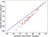 |
Fig. 1 WCS solution with the tweak order of 2 by ASTROMETRY.NET versus the real altitude from the reference catalogue of an all-sky camera image above 60° in altitude. The difference between the reference and calculated altitudes can be as large as 5°. |
2 Method
The traditional astrometric method calculates coordinates in the World Coordinate System (WCS) of an image under linear projection. When we tested the WCS solution of an all-sky camera image through ASTROMETRY.NET, as shown in Fig. 1, the difference between the reference and calculated altitudes can reach 5° above 60° in altitude, which is too large to accept. Our tests with ASTROMETRY.NET were with a tweak order of 2. Higher orders produced obvious over-fitting artefacts. Due to the non-linear projection of SWFOV images, traditional astrometric software such as S CAMP and ASTROMETRY.NET cannot be applied.
Ceplecha (1987) demonstrated astrometry on SWFOV images through an empirical model for heavily optical distorted fisheye photographs. They used a parametric model of the azimuth-zenith coordinates obtained from polar coordinates in the focal plane. The model assumes that the projection was axisymmetric and the optical centre of the image was the zenith. The azimuth a and zenith ɀ in this model are described as follows:
 (1)
(1)


Here (x, y) are the plate coordinates of a target star, (x0, y0) is the centre of the image, r is the radial distance of the star from the centre, a0 is the azimuth offset of the plate coordinates system from true north, and V, S, and D are constants describing the plate scale and radial distortion.
Borovička (1992) and Borovička et al. (1995) proposed an improved model for SWFOV images in which the optical axis is not perfectly aligned with the local zenith. In their model, the optical centre of the image (x0, y0) is different from the zenith (xc, yc), as shown in Fig. 2. The planar polar coordinates (θ, r) in Eqs. (1) and (2) in this case are no longer describing (a, ɀ), but the projection coordinates (b, u), which are spherical and based on the optical centre (x0, y0). Consider the differences between the zenith and the optical centre in azimuth and zenith are E and ϵ, respectively, then the projection coordinates (b, u) of the optical centre and the horizontal coordinates (a, ɀ) of the zenith can be converted as follows:
 (4)
(4)
Borovička et al. (1995) introduced the plate shift and inclination constants A, C, F, and adding a second exponential term to Eq. (2). Then, the projection coordinates (b, u) can be described as follows:
 (5)
(5)
![$\eqalign{ & r = C\left[ {\sqrt {{{\left( {x - {x_0}} \right)}^2} + {{\left( {y - {y_0}} \right)}^2}} + A\left( {y - {y_0}} \right)\cos \left( {F - {a_0}} \right)} \right. \cr & \,\,\,\,\,\,\,\,\,\,\,\,\,\left. { - A\left( {x - {x_0}} \right)\sin \left( {F - {a_0}} \right)} \right]. \cr} $](/articles/aa/full_html/2025/03/aa52218-24/aa52218-24-eq6.png)
In Eqs. (4)–(6), the model contains 13 constants: the plate constants (a0, x0, y0), the camera constants (A, F, C), the lens constants (V, S, D, P, Q), and the zenith offset (E, ϵ). This model can adequately model the projection and distortion of SWFOV images but is hard to solve due to the large number of constants and strongly non-linear equations.
Barghini et al. (2019) proposed a simplified model specifically for their all-sky camera. Since only a few hundred bright stars (MV < 4.5) were available for their camera and their astrometric solution did not need to be as accurate, they replaced the camera and lens parameters with known the projections of their camera. Then Eqs. (5) and (6) can be described as follows:
 (7)
(7)

In Eq. (7), F0 and R are constants depending on the projection type. For example, with an equi-solid projection, we have F0 = 2 and R = 2 f, where f is the focal length. In Eqs. (7) and (8), the number of parameters are reduced to six, with F0 and R able to be easily estimated from the known frame size and approximate radial plate scale. However, in this simplified model proposed by Barghini et al. (2019), the projection formula does not contain distortion parameters, while the residuals in |a − acat| sin (ɀcat) and |ɀ − ɀcat| are as large as 2°. Therefore, they used the full formulation by Borovička (1992) for the complete astrometric solution.
Tian et al. (2022) produced a fixed model using machine learning to estimate distortions. Machine learning can solve the problem well, but the method is not universal. Cameras with different lenses and sites require different models of machine learning, and the training process is time intensive and requires a large training set of tagged sample data.
In summary, the methods mentioned above are either hard to use to obtain a solution or do not model the distortion sufficiently accurately. This provided the motivation for us to develop a semi-analytical method for astrometry of SWFOV images with distortion. Our method here targets the distortion problem using the inversed Kannala-Brandt model, which is commonly used in estimating the photograph distortion of pinhole cameras (Kannala & Brandt 2006). As an example, Jeanne et al. (2019) used this model in detecting fireball meteor trajectories following the study of Hughes et al. (2010). The model describes the general form of projections for most types of fisheye lenses as a Taylor series:
 (9)
(9)
Assuming the optical system is axisymmetric, Eq. (9) can describe the projection and radial distortion of a SWFOV image. Taking Eq. (9) together with Eqs. (4) and (7), the final form of our method is as follows:
 (10)
(10)
In Eq. (10), the constants can be divided into three groups according to their physical meaning. The first group is the parameters of the optical centre (x0, y0). The second group is the zenith parameters (a0, E, ϵ), referring to the deviation of the camera optical axis from the zenith. The third group is the distortion parameters (kn), describing the projection and distortion of the camera.
Compared with the previous works (Ceplecha 1987; Borovička et al. 1995; Barghini et al. 2019; Jeanne et al. 2019; Tian et al. 2022), our method takes into account the difference between the optical centre and zenith, converts the plate coordinates (x, y) to horizontal coordinates (a, ɀ) with fewer parameters, and obtains the radial distortion semi-analytically. Most importantly, we provide a practical implementation in Sect. 4 for others to use with their own data.
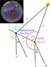 |
Fig. 2 Celestial sphere diagram showing the deviation of the optical centre from the zenith and a target star in a different coordinate system. It is presented in plane rather than spherical projection for easier viewing. In the upper left, a sketch shows the location of the optical centre and the zenith relative to the whole image. The optical centre (x0, y0) is slightly off the zenith (xc, yc), and the parameters (E, ϵ) refer to the deviation in azimuth and zenith, respectively. The planar polar coordinates (θ, r) and spherical projection coordinates (b, u) are based on the optical centre (x0, y0), while the horizontal coordinates (a, ɀ) are based on the zenith (xc, yc). N is true north, whereas n is the direction of the initial ray of the polar coordinates (where θ = 0°); a0 is their difference in azimuth. |
3 Instrument and data
To implement our method described in Sect. 2, we used the data from the all-sky camera KLCAM as an example. KLCAM is deployed in Dome A, Antarctica, to monitor the cloud cover and aurora contamination. We analysed the 2017–2018 KLCAM data and obtained the a clear-sky fraction for Dome A of roughly 83 per cent (Yang et al. 2021). Together with other site testing results such as the extremely good seeing (Ma et al. 2020), this shows that Dome A has the best observing conditions for ground-based optical astronomy (Shang 2020).
3.1 KLCAM
The detailed design of KLCAM can be found in Shang et al. (2018). Here we briefly present the basic features of KLCAM.
KLCAM is equipped with a Sigma 4.5 mm f/2.8 fisheye lens and a Canon 100D camera. The camera sensor is a 22.3 × 14.9 mm Complementary Metal Oxide Semiconductor (CMOS) with a pixel size of 4.29 µm, which gives KLCAM a 180° FOV with a pixel scale of roughly 3.5′/pixel. As the projection of KLCAM is equi-solid, the pixel scale changes through the radial direction. Figure 3 shows the appearance and thermal design of KLCAM; the camera and lens along with the controlling computer are integrated inside the enclosure. The thermal design guarantees that KLCAM works perfectly at the extremely low ambient temperatures of −80 °C at Dome A. The power of KLCAM is supplied by the PLATeau Observatory for Dome A (PLATO-A; Ashley et al. 2010), a self-contained automated platform designed for operation in Antarctica.
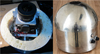 |
Fig. 3 KLCAM in laboratory. Left: Fisheye lens and the camera set on an isothermal frame with the controlling computer inside and surrounded by a layer of thermal insulation. Right: Metal enclosure of KLCAM with the lens on the top of the hemisphere. |
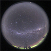 |
Fig. 4 Nighttime KLCAM image captured in 2017 May showing the bright stars, the Milky Way, and the Large and the Small Magellanic clouds. The green and red aurorae can be seen around the horizon. |
3.2 Data
Since installed at Dome A in 2017 January, KLCAM has worked for 490 days. A total of 47 035 images were collected at an exposure interval of 30 minutes. In this work we used the nighttime data from 2017, totalling 5170 images. The exposure time of KLCAM was set to 30 seconds at night. Figure 4 shows a typical image of KLCAM.
The Canon 100D camera takes images with a Bayer filter, which has a colour pattern of RGGB (Fig. 5). Each colour channel of the camera takes only one-quarter of the pixels of the full image. This leads to the image size of a single colour channel being reduced from 5184 × 3456 pixels to 2592 × 1728 pixels, and the pixel scale being reduced to roughly 7′. The data were saved in the Canon CR2 RAW image format. For further analysis, we converted the data to four-channel Flexible Image Transport System (FITS) images using a PYTHON script based on RAWPY1 and LIBRAW2. We used the G-band images for further analysis since this band is closest to the Bessel V band.
 |
Fig. 5 Sketch of the Bayer filter colour pattern. The pixels were divided into RGGB four-colour channels, and each channel takes one-quarter of the pixels of the image. Coloured photographs are usually reconstructed to their original size via interpolation. However, we prefer not to use interpolation to prevent unreal values. |
4 Implementation
Our method described in Eq. (10) requires at least nine constants to be estimated (Sect. 2). However, each parameter has a physical meaning and some will remain fixed for all images. We give below an example of solving for the constants using a KLCAM all-sky image. The PYTHON code we used is published on GIT-HUB3.
4.1 Step 1: Finding positions of stars and the initial optical centre
In this step, we obtain the (x, y) positions of the stars in the images and find the initial optical centre (x0,ini, y0,ini). To produce a star catalogue, we used SOURCE EXTRACTOR (Bertin & Arnouts 1996) to perform basic photometry on the FITS images we presented in Sect. 3.2. The catalogue contains not only (x, y) positions, but also instrumental magnitudes, full widths at half maximum, and elongations of the stars. The full widths at half maximum and elongations can help remove false signals, while the instrumental magnitude is useful when cross-matching the stars with a reference catalogue.
To estimate the initial optical centre (x0,ini, y0,ini), we used the PYTHON script based on the function CV2.HOUGHCIRCLE4 and a daytime image (Fig. 6). By image recognition, the script can find the centre of the circular exposure region, which is the optical centre of KLCAM. For the initial optical centre, any other method is acceptable as long as the error is not greater than, empirically, 10 pixels. A more precise value will be obtained later.
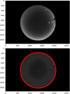 |
Fig. 6 Initial optical centre estimated using the centre of the circular exposure region with a PYTHON script based on the function CV2.HOUGHCIRCLE. The upper panel is the image captured during the daytime, and the lower panel shows the circle and the centre in red. Our estimate of the centre is only approximate since the image has structures around the horizon that will bias the result. |
4.2 Step 2: Initial astrometric solution for a single image
After the positions of stars and the initial optical centre are obtained, we cross-matched the brightest stars in one template image and then estimated the initial zenith parameters (a0,ini, Eini, ϵini) and the initial distortion parameters (kn,ini). The initial matching of (x, y) → (a, ɀ) can be obtained manually or through empirical polynomial fittings. Since this step only needs to be done once and we only need a few of the brightest stars, we manually identified stars brighter than 2.5 Vmag at different altitude and azimuth. As Fig. 7 shows, we identified 50 stars from the image in the reference catalogue. We used the Tycho-II catalogue (Høg et al. 2000) in the V band as the reference catalogue and obtain their (aref, ɀref) from (RA, Dec) along with the observation time and site location. This process is straightforward and fast. However, if the camera is moved or anything changes, the manual identification needs to be redone as the visible constellations change with observing time.
The initial zenith parameters (a0,ini, Eini, ϵini) can be estimated through Eqs. (4), (7), and (8), using known projection parameters F0 and R for a specific camera and lens. Based on the equi-solid projection type, the focus of 4.5 mm, and the pixel size of 216.7 pixel/mm, we can obtain that F0 = 2 and R = 975 in Eq. (7). For commercial cameras such as that used in KLCAM, the F0 and R from the parameter table are not particularly accurate, but we only need an approximation to obtain the initial value here.
Using the (x, y) positions of stars, the referenced horizontal coordinates (aref, ɀref), the optical centre (x0,ini, y0,ini), and parameters F0 and R, we can obtain the zenith parameters (a0,ini, Eini, ϵini) by fitting Eqs. (4), (7), and (8). At this point we could insert the parameters found above into Eq. (10) and estimate the initial distortion parameters (kn,ini) by fitting. We used the fourth-order approximation of distortion parameters, which is accurate enough and can be solved both in (a, ɀ) → (x, y) and (x, y) → (a, ɀ). We iterated the fitting process in estimating parameters (a0,ini, Eini, ϵini) and (kn,ini) ten times to obtain the initial solution.
Based on the initial solution, we could then calculate the (a, ɀ) coordinates of the stars and compare them with the reference catalogue. As Fig. 8 shows, the residual of calculated (acal, ɀcal) and reference (aref, ɀref) is within 0.25°. As the pixel scale is roughly 7′/pixel, the residual is within roughly 2 pixels. The initial solution is not very precise, but it is sufficient to use to automate the cross-matching of bright stars with the reference catalogue. By testing, we find that the initial number of manually matched stars can be as few as 25 provided they are fairly evenly distributed across the image.
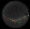 |
Fig. 7 The 50 stars identified in the KLCAM image. The stars were manually cross-matched with the reference catalogue. |
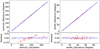 |
Fig. 8 Left: calculated azimuth versus the referenced one, and the O–C residual. Right: same but in zenith. The solution is based on 50 stars. |
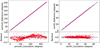 |
Fig. 9 Left: calculated azimuth versus the referenced one, and the O–C residual. Right: same but in zenith. The solution is based on roughly 700 stars. |
4.3 Step 3: Iterated solution with more stars
In the final step, we used more stars to obtain the final result by iterating step 2. Using the (x, y) of stars obtained in step 1, and the initial solution obtained in step 2, we could calculate the (a, ɀ) using Eq. (10) and then convert it to (RA, Dec) based on the observation time and site location. We used a PYTHON script based on the function of ASTROPY.COORDINATES (Astropy Collaboration 2013, 2018, 2022) to cross-match the stars with the reference catalogue.
After the cross-matching, we could fit our instrumental magnitude using a simple zero-point, and we used this to assist with verifying the match of stars with the catalogue. We restricted ourselves to using stars brighter than 5.5 Vmag, which left us with roughly 700 usable stars. We iterated step 2 based on these 700 stars, and the Observed-minus-Calculated (O–C) residuals of the result are shown in Fig. 9.
This is clearly a sinusoidal signal in the azimuth residuals (Fig. 9). This is dominated by the inaccurate positioning of the optical centre, as the optical centre has been only roughly estimated at this stage. We developed a method to improve the accuracy of the optical centre. Firstly, we used the amplitude of the sinusoidal signals in the residual of azimuth as the indicator to estimate the accuracy of the optical centre. Then, we moved the position of the optical centre in a 10 × 10 pixels squares around the initial optical centre. Each time we moved the position, we calculated the residual of azimuth and found the smallest amplitude of the sinusoidal signals, which is supposed to be the closest position of the real optical centre.
As Fig. 10 shows, each point refers to an amplitude of the sinusoidal signal calculated with each optical centre candidate. Finally, we found the best position through two-dimensional fitting.
After the improved optical centre is obtained, we iterated step 2 again to obtain the final solution, and the residuals of the result are shown in Fig. 11. The root-mean-square (RMS) error of ∆ɀ is 3.58′, and the RMS of ∆a sin ɀ is 2.03′. We also converted the (RAref, Decref) to ( xref, yref) and obtained the RMS error in (x, y) positions. As Fig. 12 shows, the errors are 0.44 pixels in x and 0.38 pixels in y, which is accurate enough for further study in site testing and possible photometry.
4.4 Statistical results on 5170 images
We applied our final solution to all the 2017 KLCAM data. Figure 13 shows the statistical result of both the RA and Dec astrometry errors. The mode numbers of RA and Dec errors are 2.75′ and 3.75′, respectively. The median numbers are 3.04′ and 3.91′. The result shows that our method is stable when applied to massive datasets. Once the solution is built, our method can be applied to every single image as long as the camera does not move or the hardware does not change.
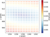 |
Fig. 10 Result of the centre fitting. Each point is a centre position, while x, y are in pixels. The colour of each point refers to the amplitude, A, of the sinusoidal signal calculated with the exact centre. Theoretically, the optical centre is located where A = 0. We used two-dimensional fitting to find the best centre position. |
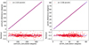 |
Fig. 11 Left: calculated azimuth versus the referenced one, and the O–C residual. Right: same but in zenith. The calculated azimuth and zenith are based on the final solution. The σ of the zenith is calculated from ∆ɀ, while the residual of azimuth is calculated from ∆a sin ɀ. |
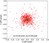 |
Fig. 12 Positional differences between the observed stars and reference catalogue in (x, y). The RMS errors in (x, y) are 0.44 and 0.38 pixels, respectively. The green circle in the middle marks the optical centre. |
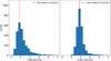 |
Fig. 13 Statistical result of the final solution applied to all 2017 KLCAM images, showing the histogram of the fitting errors of RA (left) and Dec (right) in arcminutes. The mode numbers are 2.75′ and 3.75′ for RA and Dec, respectively. |
5 Discussion and conclusion
We have developed a universal astrometry method for SWFOV images (see Sect. 2) and applied it to data from the all-sky camera KLCAM as an example (see Sect. 4). The method can be used on data from different all-sky cameras at different sites following the steps that we have outlined.
Since the method is relatively accurate and semi-analytically solvable, it can be used for astrometry, and subsequent photometry, of all-sky camera images. The photometry comparison with reference cloud-free images enables automatic real-time cloud detection, which is useful for the scheduling of observations and future artificial intelligent observatories.
Furthermore, the method is not only for all-sky cameras but also for all SWFOV images. For cameras with different projection types, our method can be applied using an appropriate choice of parameters in the distortion equation. The only prerequisite is that the images are axisymmetric.
One aspect not considered here is the effect of trailing of star images in long unguided exposures, which reduces the accuracy with which the star positions can be determined. This problem is mitigated somewhat with KLCAM images due to the latitude of Dome A placing the south celestial pole near the zenith. However, sites at lower latitudes should take the effect into consideration and use appropriate shorter exposure times.
A final consideration is the possible need to take atmospheric differential refraction into account. This can be done by correcting the catalogue star positions for refraction before using them in the fitting process. The refraction correction can be based on a model such as PYERFA5, which would require on-site air pressure, temperature, relative humidity, and average wavelength information. Alternatively, for all-sky images where the optical axis is close to the zenith, sufficient accuracy can probably be obtained by incorporating the refraction correction into the distortion correction.
In conclusion, we have developed a generalized astrometry method for SWFOV images and implemented the method with the all-sky camera KLCAM.
The method is semi-analytically solvable with sub-pixel accuracy;
As an example, we applied our method in a three-step process with an all-sky camera image, obtaining residuals of 0.44 pixels in x and 0.38 pixels in y, corresponding to 2.03′ in RA and 3.58′ in Dec;
We applied our method to all 5170 images, and the statistical mode numbers of RA and Dec are 2.75′ and 3.75′, respectively, showing the stability of our method;
Our method is generalized and can be applied to any SWFOV image, and we provide our code on GitHub as a practical implementation so that others can use it with their own data.
Acknowledgements
We thank the CHINARE for their great efforts in installing KLCAM, maintaining KLCAM and PLATO-A, and retrieving data. This work has been supported by Beijing Natural Science Foundation under Grant No. 1244060, the National Key Research and Development Program of China under Grant No. 2023YFA1608301, the Strategic Priority Research Program of the Chinese Academy of Sciences under Grant No. XDB0550101, the National Natural Science Foundation of China under Grant Nos. 12373092, 12133010, 11873010, 11733007, 11673037, 11403057, and 11403048, the Chinese Polar Environment Comprehensive Investigation and Assessment Programmes under grant No. CHINARE2016-02-03, and the National Basic Research Program of China (973 Program) under Grant No. 2013CB834900. PLATO-A is supported by the Australian Antarctic Division.
References
- Ashley, M. C. B., Allen, G., Bonner, C. S., et al. 2010, in EAS Publications Series, 40, eds. L. Spinoglio, & N. Epchtein, 79 [NASA ADS] [CrossRef] [EDP Sciences] [Google Scholar]
- Astropy Collaboration (Robitaille, T. P., et al.) 2013, A&A, 558, A33 [NASA ADS] [CrossRef] [EDP Sciences] [Google Scholar]
- Astropy Collaboration (Price-Whelan, A. M., et al.) 2018, AJ, 156, 123 [Google Scholar]
- Astropy Collaboration (Price-Whelan, A. M., et al.) 2022, ApJ, 935, 167 [NASA ADS] [CrossRef] [Google Scholar]
- Barghini, D., Gardiol, D., Carbognani, A., & Mancuso, S. 2019, A&A, 626, A105 [EDP Sciences] [Google Scholar]
- Bertin, E. 2006, in Astronomical Data Analysis Software and Systems XV, eds. C. Gabriel, C. Arviset, D. Ponz, & S. Enrique, Astronomical Society of the Pacific Conference Series, 351, 112 [NASA ADS] [Google Scholar]
- Bertin, E., & Arnouts, S. 1996, A&AS, 117, 393 [NASA ADS] [CrossRef] [EDP Sciences] [Google Scholar]
- Bellm, E. C., Kulkarni, S. R., Graham, M. J., et al. 2019, PASP, 131, 018002 [Google Scholar]
- Borovička, J. 1992, Publ. Astron. Inst. Czech. Acad. Sci., 79 [Google Scholar]
- Borovička, J., Spurny, P., & Keclikova, J. 1995, A&AS, 112, 173 [Google Scholar]
- Borovička, J., Spurný, P., & Shrbený, L. 2022a, A&A, 667, A158 [NASA ADS] [CrossRef] [EDP Sciences] [Google Scholar]
- Borovička, J., Spurný, P., Shrbený, L., et al. 2022b, A&A, 667, A157 [NASA ADS] [CrossRef] [EDP Sciences] [Google Scholar]
- Burggraaff, O., Talens, G. J. J., Spronck, J., et al. 2018, A&A, 617, A32 [NASA ADS] [CrossRef] [EDP Sciences] [Google Scholar]
- Ceplecha, Z. 1987, Bull. Astron. Inst. Czech., 38, 222 [NASA ADS] [Google Scholar]
- Colas, F., Zanda, B., Bouley, S., et al. 2020, A&A, 644, A53 [EDP Sciences] [Google Scholar]
- Devillepoix, H. A. R., Bland, P. A., Sansom, E. K., et al. 2019, MNRAS, 483, 5166 [NASA ADS] [CrossRef] [Google Scholar]
- Dorval, P., Talens, G. J. J., Otten, G. P. P. L., et al. 2020, A&A, 635, A60 [NASA ADS] [CrossRef] [EDP Sciences] [Google Scholar]
- Gardiol, D., Cellino, A., & Di Martino, M. 2016, in International Meteor Conference Egmond, the Netherlands, 2–5 June 2016, eds. A. Roggemans, & P. Roggemans, 76 [Google Scholar]
- Hjorth, M., Albrecht, S., Talens, G. J. J., et al. 2019, A&A, 631, A76 [NASA ADS] [CrossRef] [EDP Sciences] [Google Scholar]
- Høg, E., Fabricius, C., Makarov, V. V., et al. 2000, A&A, 355, L27 [Google Scholar]
- Howie, R. M., Paxman, J., Bland, P. A., et al. 2017a, Exp. Astron., 43, 237 [Google Scholar]
- Howie, R. M., Paxman, J., Bland, P. A., et al. 2017b, Meteor. Planet. Sci., 52, 1669 [NASA ADS] [CrossRef] [Google Scholar]
- Hughes, C., Denny, P., Jones, E., & Glavin, M. 2010, Appl. Opt., 49, 3338 [NASA ADS] [CrossRef] [Google Scholar]
- Jeanne, S., Colas, F., Zanda, B., et al. 2019, A&A, 627, A78 [EDP Sciences] [Google Scholar]
- Kannala, J., & Brandt, S. 2006, IEEE Trans. Pattern Anal. Mach. Intell., 28, 1335 [CrossRef] [Google Scholar]
- Lang, D., Hogg, D. W., Mierle, K., Blanton, M., & Roweis, S. 2010, AJ, 139, 1782 [Google Scholar]
- Ma, B., Shang, Z., Hu, Y., et al. 2020, Nature, 583, 771 [NASA ADS] [CrossRef] [Google Scholar]
- Masci, F. J., Laher, R. R., Rusholme, B., et al. 2019, PASP, 131, 018003 [Google Scholar]
- Shang, Z. 2020, Res. Astron. Astrophys., 20, 168 [NASA ADS] [CrossRef] [Google Scholar]
- Shang, Z., Hu, K., Yang, X., et al. 2018, SPIE Conf. Ser., 10700, 1070057 [NASA ADS] [Google Scholar]
- Talens, G. J. J., Albrecht, S., Spronck, J. F. P., et al. 2017a, A&A, 606, A73 [NASA ADS] [CrossRef] [EDP Sciences] [Google Scholar]
- Talens, G. J. J., Spronck, J. F. P., Lesage, A. L., et al. 2017b, A&A, 601, A11 [NASA ADS] [CrossRef] [EDP Sciences] [Google Scholar]
- Talens, G. J. J., Justesen, A. B., Albrecht, S., et al. 2018, A&A, 612, A57 [NASA ADS] [CrossRef] [EDP Sciences] [Google Scholar]
- Tian, J. F., Ge, L., Wu, Y., & Zhou, Z. Z. 2022, PASP, 134, 035002 [NASA ADS] [CrossRef] [Google Scholar]
- Trigo-Rodriguez, J. M., Fabregat, J., Llorca, J., et al. 2001, WGN, J. Int. Meteor Organ., 29, 139 [NASA ADS] [Google Scholar]
- Yang, X., Shang, Z., Hu, K., et al. 2021, MNRAS, 501, 3614 [NASA ADS] [CrossRef] [Google Scholar]
All Figures
|
Fig. 1 WCS solution with the tweak order of 2 by ASTROMETRY.NET versus the real altitude from the reference catalogue of an all-sky camera image above 60° in altitude. The difference between the reference and calculated altitudes can be as large as 5°. |
| In the text | |
|
Fig. 2 Celestial sphere diagram showing the deviation of the optical centre from the zenith and a target star in a different coordinate system. It is presented in plane rather than spherical projection for easier viewing. In the upper left, a sketch shows the location of the optical centre and the zenith relative to the whole image. The optical centre (x0, y0) is slightly off the zenith (xc, yc), and the parameters (E, ϵ) refer to the deviation in azimuth and zenith, respectively. The planar polar coordinates (θ, r) and spherical projection coordinates (b, u) are based on the optical centre (x0, y0), while the horizontal coordinates (a, ɀ) are based on the zenith (xc, yc). N is true north, whereas n is the direction of the initial ray of the polar coordinates (where θ = 0°); a0 is their difference in azimuth. |
| In the text | |
|
Fig. 3 KLCAM in laboratory. Left: Fisheye lens and the camera set on an isothermal frame with the controlling computer inside and surrounded by a layer of thermal insulation. Right: Metal enclosure of KLCAM with the lens on the top of the hemisphere. |
| In the text | |
|
Fig. 4 Nighttime KLCAM image captured in 2017 May showing the bright stars, the Milky Way, and the Large and the Small Magellanic clouds. The green and red aurorae can be seen around the horizon. |
| In the text | |
|
Fig. 5 Sketch of the Bayer filter colour pattern. The pixels were divided into RGGB four-colour channels, and each channel takes one-quarter of the pixels of the image. Coloured photographs are usually reconstructed to their original size via interpolation. However, we prefer not to use interpolation to prevent unreal values. |
| In the text | |
|
Fig. 6 Initial optical centre estimated using the centre of the circular exposure region with a PYTHON script based on the function CV2.HOUGHCIRCLE. The upper panel is the image captured during the daytime, and the lower panel shows the circle and the centre in red. Our estimate of the centre is only approximate since the image has structures around the horizon that will bias the result. |
| In the text | |
|
Fig. 7 The 50 stars identified in the KLCAM image. The stars were manually cross-matched with the reference catalogue. |
| In the text | |
|
Fig. 8 Left: calculated azimuth versus the referenced one, and the O–C residual. Right: same but in zenith. The solution is based on 50 stars. |
| In the text | |
|
Fig. 9 Left: calculated azimuth versus the referenced one, and the O–C residual. Right: same but in zenith. The solution is based on roughly 700 stars. |
| In the text | |
|
Fig. 10 Result of the centre fitting. Each point is a centre position, while x, y are in pixels. The colour of each point refers to the amplitude, A, of the sinusoidal signal calculated with the exact centre. Theoretically, the optical centre is located where A = 0. We used two-dimensional fitting to find the best centre position. |
| In the text | |
|
Fig. 11 Left: calculated azimuth versus the referenced one, and the O–C residual. Right: same but in zenith. The calculated azimuth and zenith are based on the final solution. The σ of the zenith is calculated from ∆ɀ, while the residual of azimuth is calculated from ∆a sin ɀ. |
| In the text | |
|
Fig. 12 Positional differences between the observed stars and reference catalogue in (x, y). The RMS errors in (x, y) are 0.44 and 0.38 pixels, respectively. The green circle in the middle marks the optical centre. |
| In the text | |
|
Fig. 13 Statistical result of the final solution applied to all 2017 KLCAM images, showing the histogram of the fitting errors of RA (left) and Dec (right) in arcminutes. The mode numbers are 2.75′ and 3.75′ for RA and Dec, respectively. |
| In the text | |
Current usage metrics show cumulative count of Article Views (full-text article views including HTML views, PDF and ePub downloads, according to the available data) and Abstracts Views on Vision4Press platform.
Data correspond to usage on the plateform after 2015. The current usage metrics is available 48-96 hours after online publication and is updated daily on week days.
Initial download of the metrics may take a while.