| Issue |
A&A
Volume 695, March 2025
|
|
|---|---|---|
| Article Number | A14 | |
| Number of page(s) | 13 | |
| Section | Interstellar and circumstellar matter | |
| DOI | https://doi.org/10.1051/0004-6361/202451729 | |
| Published online | 28 February 2025 | |
Investigating chemical variations between interstellar gas clouds in the solar neighbourhood
1
Department of Astronomy, University of Geneva,
Chemin Pegasi 51,
Versoix,
Switzerland
2
European Southern Observatory,
Karl-Schwarzschild-Str. 2,
85748
Garching,
Germany
3
Université Claude Bernard Lyon 1, Centre de Recherche Astrophysique de Lyon UMR5574,
9 Av. Charles André,
69230
Saint-Genis-Laval,
France
4
French-Chilean Laboratory for Astronomy (FCLA), CNRS-IRL3386,
U. de Chile, Camino el Observatorio 1515,
Casilla 36-D,
Santiago,
Chile
5
European Southern Observatory,
Alonso de Córdova 3107, Vitacura, Casilla 19001,
Santiago,
Chile
6
Department of Astrophysical Sciences, Princeton University,
Princeton,
NJ
08544-1001,
USA
7
AURA for ESA, Space Telescope Science Institute,
3700 San Martin Drive,
Baltimore,
MD
21218,
USA
8
Department of Physics & Astronomy, Johns Hopkins University,
3400 N. Charles Street,
Baltimore,
MD
21218,
USA
9
Institute of Astronomy, Kharkiv National University,
4 Svobody Sq.,
Kharkiv
61022,
Ukraine
★ Corresponding author; tanita.ramburuth-hurt@unige.ch
Received:
31
July
2024
Accepted:
31
January
2025
The interstellar medium (ISM) is a fundamental component of the Milky Way. Studying its chemical composition and the level of its chemical diversity gives us insight into the evolution of the Milky Way and the role of gas in the Galactic environment. In this study we used a novel simulation technique to model the distribution of total hydrogen between gas components and, therefore, derive new constraints on the dust depletion and metallicity. We studied individual gas components along the lines of sight towards eight bright O/B stars within 1.1 kpc of the Sun using high-resolution HST/STIS absorption spectra (R ∼ 114 000). We measured the level of dust depletion for these individual components and find components with higher levels of dust depletion compared to Milky Way sightlines in the literature. We find large ranges in the level of dust depletion among components along lines of sight, up to a factor of 15 (or 1.19 dex). Although it is not possible to directly measure the metallicity of individual components due to the saturated and damped Lyman-α line, we investigated possible metallicity ranges for individual gas components by exploring many different distributions of the total hydrogen gas between components. We selected possible combinations of these gas fractions that produce the minimum metallicity difference between components, and for these cases we determine individual metallicities to accuracies that range between ∼ 0.1 and 0.4 dex. This work shows that full line-of-sight analyses do not capture the level of diversity along lines of sight, and that component-by-component studies give a more in-depth understanding of the chemical intricacies of the ISM.
Key words: Galaxy: abundances / Galaxy: general / local insterstellar matter / solar neighborhood
© The Authors 2025
 Open Access article, published by EDP Sciences, under the terms of the Creative Commons Attribution License (https://creativecommons.org/licenses/by/4.0), which permits unrestricted use, distribution, and reproduction in any medium, provided the original work is properly cited.
This article is published in open access under the Subscribe to Open model. Subscribe to A&A to support open access publication.
1 Introduction
Studies of the chemical composition of the Milky Way’s interstellar medium (ISM) give us important insight into its evolution and the role of gas in the Galactic environment. Determining the level of diversity in the metallicity of the warm neutral gas in the solar neighbourhood is important for finding evidence of low-metallicity gas infall onto the Milky Way, for example from high-velocity clouds (Richter 2017; Fox et al. 2019). Low- metallicity gas inflows from the circumgalactic medium have been predicted in simulations (Schaye et al. 2015; Crain et al. 2015; Nelson et al. 2019; Pillepich et al. 2019; Péroux et al. 2020). Evidence of pockets of low-metallicity gas in the ISM of the Milky Way could be an indication of low-metallicity gas infall (De Cia et al. 2021).
Absorption-line spectroscopy is a powerful method for studying the metal content of the gas in galaxies because it gives access to the column densities of many metals (ions), and the methods of measuring the column densities are robust. Additionally, UV absorption-line spectroscopy is particularly valuable because the resonant lines of the most dominant ionisation states of the most abundant cosmic metals (O, C, Fe, Si, etc.) are available in the UV. There are several phenomena to take into account when calculating the total overall metallicity (i.e. gas plus dust), including dust depletion, ionisation effects, and nucleosynthesis effects.
Dust depletion is the phenomenon whereby metals are incorporated into dust grains and are no longer observable in the gas phase (Field 1974; Phillips et al. 1982; Jenkins et al. 1986; Savage & Sembach 1996; Jenkins 2009; De Cia et al. 2016, 2021; Roman-Duval et al. 2021; Konstantopoulou et al. 2022). The depletions of different metals correlate with each other to varying degrees depending on how easily they form dust. The tendency of a metal to deplete into dust is called its refractory index, and it is broadly correlated to the condensation temperature of the metal (Savage & Sembach 1996; De Cia et al. 2016; Konstantopoulou et al. 2022). Metals that form dust more readily are referred to as refractory, while those that form dust lesseasily are volatile. The measure of the relative abundances between metals with different refractory properties is therefore a measurement of the amount of dust depletion. In this method for characterising dust depletion, called the ‘relative method’ (De Cia et al. 2016, 2021; Konstantopoulou et al. 2022), the determination of the refractory indices of metals is based on the relative abundances of Zn and Fe. An advantage of the relative method is that it does not make any assumption on the metallicity of the gas.
In addition to dust depletion, there are at least two other phenomena that can affect the abundances of metals: ionisation and nucleosynthesis effects. In general, the ions in the warm neutral ISM of the Milky Way are singly ionised (with the exception of O I) and are not highly susceptible to further ionisation because they are protected from ionising radiation by neutral hydrogen H I. Elements that are further ionised from ionisation potentials higher than that of H I (13.6 eV) can also survive in H II regions, which could result in their apparent over-abundance. For example, as shown in Jenkins (2009), the second ionisation potential of S is higher than that of most other elements, meaning that it can be present in a broader range of H II regions (i.e. where the radiation field is harder and many other elements will be doubly ionised), so it is more likely for it to have contributions from H II regions than most other singly ionised species. Nucleosynthesis effects, for example α- element enhancement and Mn under-abundance, may also affect observed metal abundances. Although α-element enhancements are observed in the Magellanic Clouds (De Cia et al. 2024) and in distant gas-rich galaxies (Velichko et al. 2024), they are not generally seen in the Milky Way.
In most cases, chemical enrichment and metallicities in the neutral ISM are determined for the whole line of sight towards stellar targets in the Milky Way (e.g. Jenkins 2009; De Cia et al. 2021; Ritchey et al. 2023). Itis possible that intricacies at smaller scales, at the level of individual gas components along the lines of sight, make the ISM more complex at this level, and that by studying whole lines of sight we overlook small-scale chemical variations. Evidence of this comes from deviations from the normal abundance patterns (the distribution of the observed ![$[X/{\rm{H}}] = \log {{N(X)} \over {N(H)}} - \log {{N\left( {{X_ \odot }} \right)} \over {N\left( {{H_ \odot }} \right)}}$](/articles/aa/full_html/2025/03/aa51729-24/aa51729-24-eq1.png) against their refractory index for different metals). In these cases, volatile elements seem to deviate from the more typical linear shape of abundance patterns. A possible explanation for these abnormal abundance patterns is that the gas along the lines of sight is a mix of low- and high-depletion gas and/or high- and low-metallicity gas.
against their refractory index for different metals). In these cases, volatile elements seem to deviate from the more typical linear shape of abundance patterns. A possible explanation for these abnormal abundance patterns is that the gas along the lines of sight is a mix of low- and high-depletion gas and/or high- and low-metallicity gas.
With high-resolution absorption-line spectroscopy it is possible to dissect lines of sight, and identify and study the chemical properties of individual gas components (Welty et al. 2020; Ramburuth-Hurt et al. 2023). This allows for a more comprehensive analysis of the variation (if any) in chemical enrichment between different gas clouds along lines of sight. A limitation of the component-by-component analysis is that it is not possible to know the H column density for individual components due to the Lyman-α line being damped and, therefore, too broad for the separation of individual components. This means it is not possible to directly measure the metallicity of individual components of [M/H]i. It is still possible to characterise the chemical enrichment of individual components using dust depletion as a proxy (e.g. Welty & Crowther 2010; Ramburuth-Hurt et al. 2023). However, although the level of dust depletion has some dependence on metallicity, it also depends on physical conditions, such as temperature and density. In high-pressure, high-density, and low-temperature gas, such as in the Milky Way disk, the production of molecules and dust has a smaller dependence on metallicity (Blitz & Rosolowsky 2006; Balashev et al. 2017). This means that the distribution of dust depletion does not fully trace that of the metallicity (Draine 2003; Mattsson et al. 2014; Blitz & Rosolowsky 2006; Balashev et al. 2017).
In this work, we studied the dust depletion in individual gas components along eight lines of sight in the solar neighbourhood with high-resolution UV spectra from the Space Telescope Imaging Spectrograph (STIS) on the Hubble Space Telescope (HST). We present a novel methodology of investigating and constraining the metallicities for these individual components using simulations based on hydrogen gas fraction combinations. This paper is organised as follows: Section 2 introduces the data employed in this investigation, Sect. 3 elaborates on our methodology, Sect. 4 presents and discusses the findings of this study, and Sect. 5 summarises the conclusions drawn from our work.
2 Data
In this work we studied the ISM along the lines of sight towards eight bright O/B-type stars within 1.1 kpc of the Sun. These targets are a subsample of the 25 targets compiled by De Cia et al. (2021). We selected the subsample based on three main criteria:
The presence of multiple components in the Ti II absorption lines, based on spectra from the Ultraviolet and Visual Echelle Spectrograph (UVES) on the Very Large Telescope (VLT) and Kitt Peak.
An upturn of volatile elements in the abundance patterns in De Cia et al. (2021), which suggests a mix of gases of different dust depletion and/or metallicities along the line of sight.
Lower metallicity (≤ −0.16 dex according to De Cia et al. 2021) over the integrated line of sight.
While it is possible that the metallicities from De Cia et al. (2021) are underestimated with respect to other strategies (Ritchey et al. 2023), we based our sample selection on lines of sight that potentially showed signatures of low metallicity gas, which is the motivation for the third condition. The star type, distance from the Galactic centre calculated from Gaia Data Release 3 (DR3), galactic latitude (b) and longitude (l), and the extinction (AV ) for the eight targets are included in Table 1.
2.1 HST data
The data we used in this work are primarily from the high spectral resolution (R ~ 114 000) HST/STIS programme ID 16750 of the eight bright O/B stars within 1.1 kpc of the Sun. This programme had 15 orbits in two settings: E140H with a central wavelength of 1271 Å, covering 1170–1372 Å, and E230H with a central wavelength of 2113 Å covering 1974–2251 Å. In the case of ρ Oph A, HD 206267 and HD 207198, the spectra for the E230H/2113 setting already exists in the archive. Table A.1 contains observational details of this programme including the number of orbits, exposure time and signal-to-noise ratio (S/N) for each setting. The wavelength bands were chosen to include the absorption lines for a number of transitions of interest tabulated in Table 2. We used the 1D spectra directly from the archive, which have been reduced by the standard CALSTIS pipeline.
2.2 Auxiliary data
We made use of the following data to supplement the absorption lines listed above. Specifically, because the decomposition of the lines is important for this work, the supplementary very high-resolution data are used to determine the substructure of the absorption lines.
Archival high-resolution HST/STIS spectra (R ~114 000, FWHM ~2.63 km s−1) that cover the Fell λλ 2260, 2367 lines for the targets ρ Oph A, HD 206267 (ID 16285) and HD 207198 (ID 9465).
VLT/ESPRESSO spectra (ID 0102.C-0699(A), R ~ 190 000, FWHM ~1.54 km s−1) that cover Ca II λλ 3934, 3969, KI λλ 7664, 7698, and Na I λλ 5889, 5895.
Kitt Peak National Observatory (KPNO) spectra from the Coude Feed Telescope with Camera 6 (R ~ 220 000, FWHM ~1.35 km s−1) that cover Ca II λ 3934 and K I λλ 7664, 7698, and from the Coude Feed Telescope with Camera 5 (R ~ 88 000, FWHM ~3.4 km s−1) that covers Ti II λ3384.
McDonald spectra (R ~ 176 000, FWHM ~1.7 km s−1) that cover K I λλ 7664, 7698 and Ca II λλ 3934, 3969 (Pan et al. 2004).
Ultra High Resolution Facility (UHRF) spectra covering NaI λλ 5889, 5895, K I λ7698 (Welty & Hobbs 2001) and CaII λλ 3934, 3969 (R ~ 880 000, FWHM ~0.34; Price et al. 2001).
VLT/UVES spectra (ID 194.C-0833, R ~ 92 600, FWHM ~3.2 km s−1) that cover Ti II λλλ3230, 3242, 3384.
Table 2 contains the rest wavelengths, oscillator strengths, and γ values for each of the transitions we considered.
Target information with distances from the Galactic centre calculated using Gaia DR3.
Rest wavelengths, oscillator strengths and their reference for the transitions considered in this work.
3 Methodology
To analyse the chemical enrichment and variations along these lines of sight, we started by measuring column densities using Voigt-profile fitting software packages, described in Sect. 3.1. In this work we go beyond the more typical study of the abundance patterns (variations of [X/H] with the refractory index) along the full line of sight by performing a component-by- component analysis along the lines of sight. To do this, we constructed metal patterns (also called depletion patterns in Ramburuth-Hurt et al. 2023). These are the metal-to-metal variations with respect to their tendency to deplete onto dust grains, namely the refractory indices, plotted against their equivalent metal column densities (log N(X) − log N(H) for a given metal X). From these metal patterns we can pinpoint the amount of dust depletion in individual components (Sect. 3.2). We then performed simulations, based on the observations, to further constrain the possible ranges of metallicities of the individual components (Sect. 3.3). We did this by exploring many distributions of the total hydrogen gas among the components. In this section we describe this methodology in more detail and discuss some of its caveats.
3.1 Measuring column densities
The H I column densities are measured from the Lyman-α absorption line at 1215 Å by determining the radial velocity for most of the gas from the OI λ1355 line. This Is a good indicator of the velocity structure of H I because its ionisation energy is very similar to that of H I and the ionisation fractions of O I and H I are strongly coupled to each other by a charge exchangeprocess with a large rate coefficient (Stancil et al. 1999; Spirko et al. 2004). This line is also far from saturated, and oxygen is not much depleted onto dust grains. The outcome of this velocity measurement is used to establish an origin for trial HI Absorption profiles. The column density is then measured by determining the best fit damping profile for the Lyman-α line. In some cases, one side of the H I absorption profile showed sufficient cancellation of the H I absorption while the other side exhibited extra absorption. This effect could be due to some absorption by the stellar Lyman-α if the star’s velocity is displaced from that of the foreground gas. It is not easy to confirm this interpretation, however, because there is a high probability that the star could be a spectroscopic binary and therefore could exhibit this same effect. The targets with this effect are θ1 Ori C, HD 154368, HD 110432, and χ Oph. Column densities of H2 are taken from Savage et al. (1977).
We used two software packages for measuring the metal column densities for the targets in this work. For most of the targets (ρ Oph A, HD 110432, HD 154368, HD 2062676, and HD 207198) we used the Voigt-profile fitting software VoigtFit (Krogager 2018). For κ Aql, χ-Oph, and θ1 Ori C, metal column densities were measured using fits6p (Welty et al. 1991, 2003, 2020). We note that the uncertainties on the column densities for the fits with fits6p are underestimated.
For all targets, the structure of the absorption lines is determined by first fitting the lines covered by the highest-resolution spectra we have. We did this in order to best capture the intricacies of the line profiles, and because the STIS data are under-sampled (fewer than two pixels per resolution element). We assumed that all species have a common velocity structure, which is obtained from the highest resolution spectra, but with possible slight adjustments based on the UV profiles, especially in the cases of weak components or broad lines. We assumed that the component absorption lines are represented by symmetric Voigt profiles, and that asymmetry implies the presence of more than one component.
For ρ-Oph A, HD 110432, HD 154368, and HD 2062676, we used either Ca II λλ3934 or 3969 (or both simultaneously, when available). For HD 207198, the Ca II lines are saturated, and therefore cannot be used. Instead, we fitted simultaneously toCr II λλλ 2056, 2062, 2066 and Ti II λ 3384 to determine the structure. For κ Aql, χ Oph, and θ1 Ori C, we obtained a mutually consistent structure from the highest resolution KI, Na I, and Ca II spectra that were available. The b-values (which represent the distribution of velocities due to gas turbulence and thermal kinematics, with turbulence dominating in the warm neutral ISM), velocities and column densities for fits to the highest resolution data are included in Table C.1.
Once the component profile is determined, the decomposition is then assumed to be applicable to all other singly ionised species. The column densities are measured using all available (non-saturated, non-contaminated) lines from the same species according to this structure. In several cases, there is a velocity offset between the optical and UV spectra, which is taken into account when applying the velocity structure across these spectra. The spectra and fits are shown in Appendix C.
For some of the ions, it is not possible to decompose their absorption lines to the same level of intricacy as the high resolution lines because the lines are weaker and/or because of blending at lower resolutions. As a result, and to ensure the reliability of our measurements, we considered the column densities of groups of components (grouped by velocity) rather than all components individually, also because these are generally better constrained than individual components. It is important to note that the decomposition of components is not necessarily physical, and we do not know if the separation in velocity space means that they are separated in physical space. In this work we were careful to group the components using the highest-resolution spectra to identify individual components. Tables C.2–C.9 present the column densities for groups of components, including the way that the components were grouped and their respective velocity ranges. For simplicity and to avoid repetitive phrasing, we use the term ‘components’ to refer to groups of gas components for the remainder of this paper.
S II, Si II and Zn II are often saturated. We did not use the S II or Si II lines in our analysis because of their severe saturation, and did not use Zn II for HD 206267 and HD 207198. Some of the components on the edges of the Zn II absorption lines are salvageable, and we take the column densities from VoigtFit to be lower limits on the total line of sight. When there were individual components on the edges of the Zn II profiles that are unsaturated, we included them in the component-by-component analysis.
Most of the absorption lines towards ρ Oph A are saturated (see the fits in Fig. G.3). We could recover reliable column densities for the first component, but the lines for the second group of components (group 2, components 4–7) are too saturated, with the exception of Ti II and O I. Therefore, for this target, we only took Ti II and O I into account for the metal pattern of group 2. We did not perform further analysis on this line of sight.
3.2 Dust depletion of individual components
We used the relative method of characterising dust depletion where the depletion of element X, denoted as δX, is estimated from relative abundances (De Cia et al. 2016; Konstantopoulou et al. 2022), not observed abundances. Relative abundances are defined as [X/Y] = log N(X)/N(Y) − log N(X)⊙/N(Y)⊙, where the solar abundances are taken from (Asplund et al. 2021) following the recommendation of Lodders et al. (2009).
The relative method is based on full line-of-sight measurements along lines of sight in the Milky Way, Magellanic Clouds, Gamma-ray burst damped Ly-α absorbers (GRB-DLAs) and quasar DLAs (QSO-DLAs). Here we assumed that the method is applicable to the individual components that we studied based on the following. Firstly, Ramburuth-Hurt et al. (2023) demonstrate that the dust depletion sequences hold for individual components in QSO-DLAs, that is, ionisation effects are limited and the dominant effect of dust depletion can be clearly identified and studied also in individual components. However, that study did not include Milky Way lines of sight, or systems with a high level of dust depletion. This adds some level of uncertainty to this study. The line of sight towards HD 62542 in the Milky Way (Welty et al. 2020) is an example of a case where the depletion patterns in individual components may depart from the general trends. Evidence of deviations from the linear behaviour of metal patterns would provide clues that this method is not applicable to individual components in this regime. Secondly, dust depletion has been shown to behave similarly in different environments (QSO–DLAs, GRB-DLAs, the Magellanic Clouds, and the Milky Way; Konstantopoulou et al. 2022). Finally, the dust tracer [Zn/Fe] correlates with other relative abundances that are used as dust tracers, such as [Si/Ti] (De Cia et al. 2016; Konstantopoulou et al. 2024).
Most extragalactic work is based on the full line-of-sight analysis of mid/high-resolution (R < 50 000) spectra. The amount of depletion is expressed as
![${\delta _X} = A{2_X} + B{2_X} \times {[{\rm{Zn}}/{\rm{Fe}}]_{{\rm{fit}}}},$](/articles/aa/full_html/2025/03/aa51729-24/aa51729-24-eq2.png) (1)
(1)
where [Zn/Fe]fit is a measure of the overall strength of depletion, or the depletion factor; A2X and B2X are coefficients of the depletion sequence fits in Konstantopoulou et al. (2022) and are specific for each element (see Table 3). B2X is the refractory index, which represents the ease with which a metal is captured onto dust grains. Refractory elements form dust relatively readily and have more negative B2X values, while volatile elements do do not form dust so easily and have less negative B2X values. We note that A2X is typically consistent with zero within the uncertainties, and in principle it could be assumed to be equal to zero.
In general, we define the total dust-corrected metallicity of a metal X as
![${[X/{\rm{H}}]_{{\rm{tot}}}} = [X/{\rm{H}}] - {\delta _X},$](/articles/aa/full_html/2025/03/aa51729-24/aa51729-24-eq3.png) (2)
(2)
where [X/H]tot represents the total metallicity of the neutral ISM, including dust and gas, and [X/H] are the observed gas-phase abundances. For i individual gas components along a line of sight, we combine these two equations to obtain
![${y_i} = {a_i} + B{2_X} \times {[{\rm{Zn}}/{\rm{Fe}}]_{i,{\rm{fit}}}},$](/articles/aa/full_html/2025/03/aa51729-24/aa51729-24-eq4.png) (3)
(3)
which is a linear relation, yi = ai + bx, where
 (4)
(4)
![${{a_i} = {{[{\rm{M}}/{\rm{H}}]}_i} + \log N{{({\rm{H}})}_i}.}$](/articles/aa/full_html/2025/03/aa51729-24/aa51729-24-eq6.png) (5)
(5)
Here, log N(X)i, [M/H]i and log N(H)i are the metal column density, dust corrected metallicity and total hydrogen (i.e. H I + H2, ignoring the ionised hydrogen H II) column density for individual gas components along the line of sight. yi represents the ‘normalised’ (by its solar abundance) metal column densities.
We plotted the yi values for each metal against its corresponding B2X, which constitutes what we call a ‘metal pattern’ (or ‘depletion pattern’ in Ramburuth-Hurt et al. 2023) In the case where there is no dust depletion (or any other causes of deviation), yi for each metal would be similar. If there is only dust depletion at play, we would expect the yi values to align on a straight line with a gradient [Zn/Fe]fit,i, which represents the overall strength of depletion. The y-intercept of this straight line, ai = [M/H]i + log N(H)i, is the sum of the total hydrogen column density and dust-corrected metallicity of the individual gas component, and it is degenerate. To demonstrate this degeneracy, consider a line of sight with two individual components and the following two (of several possible) scenarios. If we have a1 < a2, it is possible for component 2 to either have a majority of the hydrogen and a low metallicity or have less hydrogen but a higher metallicity than component 1.
With the relative method, we characterised the level of dust depletion for individual gas components along the line of sight regardless of its hydrogen content. Deviations from the fitted linear relation are possible and could be due to processes such as ionisation or nucleosynthesis (e.g. α-element enhancement), or peculiar depletion due to local physical conditions of a gas cloud. Potential peculiarities of dust depletion were observed for the Magellanic Clouds (Jenkins & Wallerstein 2017) but are likely due to α-element enhancement (Konstantopoulou et al. 2022; De Cia et al. 2024). The relative method is able to distinguish between dust depletion, α-element enhancement, and metallicity variations.
An alternative to the relative method is the F* method (Jenkins 2009). We do not discuss this method in this paper, but we note that the values for depletion we determine here are related to the F* method by the equation F* = 1.05× [Zn/Fe]fit − 0.86 (based on data from De Cia et al. 2021).
While the metallicity of components is not possible to constrain, the dust depletion of each component is well constrained by Eq. (3). Metal patterns give us information on any variation in the amount of dust between gas clouds along a line of sight. We were able to study the dust depletion of the ISM on a component-by-component basis without making assumptions on the metallicity or the hydrogen distribution.
Coefficients of the depletion sequences for metals, X.
3.3 Simulating clouds: Exploring the metallicities of individual gas components
It can be argued that the distribution of O I can be used to give some insight into the distribution of hydrogen, both because it traces H I (due to their similar ionisation potential) and because it is not highly depleted into dust. The caveat with using the O I gas fraction as a direct tracer of the hydrogen fraction is that it makes the assumption that the metallicity of each gas component is the same. We chose not to do this here in order to avoid this assumption.
The distinctive difference between metal patterns described here and the more typical abundance patterns (the study of the observed abundances of elements with different refractory properties) is that we do not know the hydrogen column densities for individual components. Therefore, metals patterns cannot directly provide the metallicity of the component.
To investigate possible metallicities for components along our lines of sight, we performed simulations. The simulations take into account the observed column densities and then explore possible hydrogen gas distributions between the components. In practice, we used the y-intercept ai derived from the linear fit to the metal patterns, and calculated the metallicity based on different combinations of hydrogen gas fractions. Rewriting Eq. (5) gives
![${[{\rm{M}}/{\rm{H}}]_i} = {a_i} - \log \left( {{f_i} \times N{{({\rm{H}})}_{{\rm{tot}}}}} \right).$](/articles/aa/full_html/2025/03/aa51729-24/aa51729-24-eq7.png) (6)
(6)
Here, N(H)tot is the total hydrogen column density along the full line of sight, which can also be written in terms of the gas fraction:
 (7)
(7)
such that Σi fi = 1.
The hydrogen gas fraction combinations are generated as follows. In general, for m number of whole integers that add up to 100, the number of combinations is  . Here, we first generated all these possible permutations for each number of components (i.e. m = 2, 3, 4, 5). We then generated all the permutations of these and removed any duplicates. This process produces over 3 million combinations for m = 5; therefore, to optimise subsequent calculations, we randomly sampled 1 000 000 of the combinations; the number 1 000 000 was chosen because it yields enough combinations to cover the parameter space between 0% and 100% in intervals of 1%. For two to four components, we obtain 99, 4851, and 156 849, combinations, respectively, which is visualised in Fig. 1. The aim of this procedure is to have combinations that span the parameter space in intervals of 1%.
Then, for each gas fraction combination, we calculated the corresponding set of metallicities from Eq. (6), which we also refer to as a realisation. We did this for each combination of gas fractions and for each target. This gives us the possible ranges of metallicities for the components along each line of sight. In principle, each realisation is equally likely.
To investigate the minimum possible range in metallicity along each line of sight, we computed the difference between the maximum and minimum metallicity for each realisation, and extracted the realisation that produces the minimum difference. We interpret this is as the minimum possible variation in metallicity.
We tested this methodology by combining our observations towards HD 206267 with a sight line towards the Small Magellanic Cloud (SMC), which has known metallicity and log N(H I) from De Cia et al. (2024), to create a synthetic sight line. The choice of an SMC sight line is to demonstrate that our method can distinguish between the low metallicity of the SMC and the higher metallicity of the Milky Way. The test confirms that we are able to recover a 0.6 dex difference in metallicity between both the Milky Way components and the SMC (i.e. [M/H]MW1 – [M/H]SMC > 0.6 and [M/H]MW2 – [M/H]SMC > 0.6) for 5 out of 4865 most likely realisations. These 5 realisations also recover the metallicity and hydrogen gas fraction of the SMC cloud. The complete test is detailed in Appendix B.
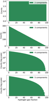 |
Fig. 1 Distributions of total hydrogen gas fractions that we used to infer the metallicities of individual components. From top to bottom: distributions for two to five components, respectively. The histograms for four and five components are plotted in log-scale for visual clarity. |
4 Results and discussion
From the analysis of the metal patterns, we derived the dust depletion of individual components and calculated the range in dust depletion along each of the eight lines of sight as the difference between the maximum and minimum depletion. We generally do not see strong evidence of deviations from the linear behaviour of the metal patterns of the individual components in this sample, and therefore assume that the relative method can be applied here. One exception to this may be the case of θ1 Ori C, where a potential overabundance of the iron-group elements or under-abundance of TiII Is observed.
We find ranges up to 1.19 dex in one case and present these results in Sect. 4.1. Using simulations, we further explored the possible metallicities and gas fractions of the individual components, which can be constrained to 0.1 dex for some lines of sight. The simulations results are presented in Sect. 4.2. We analyse the realisation that produces the minimum range in metallicity for each sight line in Sect. 4.3. In Sect. 4.4 we present the abundance patterns along the full lines of sight.
4.1 Variations in dust depletion
In our component-by-component analysis, some components show very high levels of dust depletion. The highest level of dust depletion we find is [Zn/Fe]fit,i = 2.03 ± 0.03 dex (or F* = 1.5) for group 3 in χ Oph. This value is larger than the maximum dust depletion reported by De Cia et al. (2021), which is 1.32 dex, observed towards ı Ori. Here we show the metal pattern for χ Oph in Fig. 2. In Table 4 we present [Zn/Fe]fit,i and ai for each component along each sight line. The metal patterns for the remaining targets are presented in Appendix D.
We also observe a large range in dust depletion along sight lines. Figure 3 shows that, for four of our sight lines, the difference between maximum and minimum [Zn/Fe]fit,i values reaches ~1.0 dex. For most targets, several components have significantly higher or lower levels of dust depletion compared to that of the total sight line. This result confirms that total line-of-sight analyses (e.g. De Cia et al. 2021; Ritchey et al. 2023) can wash out the level of diversity in depletion along sight lines. Indeed, it is consistent with established variations in [Na/Ca] in many Milky Way sight lines (Routly & Spitzer 1952; Siluk & Silk 1974) and with the few studies of individual components (Fitzpatrick & Spitzer 1994; Welty et al. 2020).
In Fig. 4, we plot the velocity ranges of the groups of components against their depletion. This is to investigate, firstly, any relationship between kinematics and the depletion, and secondly, any trends that could be associated with the Local Bubble (Lallement et al. 2003; Zucker et al. 2022). The Local Bubble is a pocket of plasma with low density and high temperature in which the Sun sits. Outside of the Bubble is a shell of cold, neutral gas. Zucker et al. (2022) find that several of the nearby star-forming regions sit on the edge of the Local Bubble, at a velocity of 6.7 ± 0.45 km s−1, like the Orion region. We do not find any significant relationship between velocity and depletion or any patterns, for example a systematic α-element enhancement of components around 6.7 km s−1, that could be associated with the Local Bubble. Figure 4 agrees well, however, with the velocity-depletion results of Routly & Spitzer (1952) and Siluk & Silk (1974). There may be a slight anti-correlation between absolute velocity and the level of dust depletion in these works, although we remain uncertain about the potential causes. Routly & Spitzer (1952) and Siluk & Silk (1974) interpret this as evidence of the partial destruction of dust grains within velocities of ~40 km s−1, possibly due to supernova shocks.
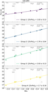 |
Fig. 2 Metal patterns for grouped components towards χ Oph. This line of sight has the highest dust depletion of our sample, with [Zn/Fe]fit,3 = 2.03 ± 0.13 dex. |
Results from the metal patterns.
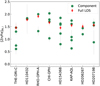 |
Fig. 3 Depletion factors for individual components along each line of sight (green points). The [Zn/Fe]fit values for the entire line of sight are plotted as red diamonds. |
4.2 Variations in metallicity
The simulations we performed produced thousands of possible metallicity combinations for individual gas components based on hydrogen gas fraction combinations, as described in Sect. 3.3. From these simulations we obtained the possible ranges of metallicities for each component (see Fig. 5 for χ Oph results). In principle, all of the realisations are equally possible because we do not state any preference for particular hydrogen gas fraction combinations. However, we did make a physically motivated upper cut on possible metallicities, which narrows the range of their possible values. The threshold is based on the maximum metallicity found in stars in the Milky Way’s disk, which Nepal et al. (2024) find to be 0.4 dex. To be conservative, we assumed that the upper limit on the gas-phase metallicity could be slightly higher and therefore imposed a limit of [M/H]i ≤ 0.5 dex. This limit decreases the range of allowed metallicities for most components, and can even constrain the possible metallicity of a component down to within an interval of ~0.3 dex including uncertainties, for example group 3 of χ Oph and group 2 of HD 110432. We show the allowed metallicities for each component along our lines of sight in Appendix E (Figs. E.1–E.5). The highlighted points in these figures indicate the realisation that produces the smallest range in metallicity. This is discussed later in Sect. 4.3.
In five lines of sight (θ1 Ori C, χ Oph, HD 154368, κ Aql, HD 207198), we find that the component with the highest [Zn/Fe]fit,i holds the majority of the hydrogen gas, and also lik- ley has super-solar metallicity. These five cases and these results are listed in Table 5. The exceptions are ρ Oph A, for which we cannot perform this analysis due to limited data, and HD 110432 and HD 206267, which both have two components of the same [Zn/Fe]fit,i within the uncertainties. Below we further discuss the results of the most likely realisations for some of the targets.
Five sight lines where the component with the highest depletion also contains the majority of the hydrogen gas.
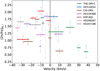 |
Fig. 4 Velocity-depletion plot for groups of components. |
4.2.1 θ1 Ori C
In addition to group 2 having high depletion, this component has super-solar metallicity and the bulk of the hydrogen gas (see Fig. 6). Additionally, there is evidence that this gas cloud is attributed to the gas Orion nebula itself (Price et al. 2001). We also find that group 4 has the lowest amount of dust depletion, sub-solar metallicity, and ≤40% of the hydrogen gas.
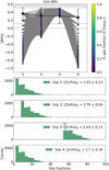 |
Fig. 5 Simulation realisations for the most likely cases (where the metallicities for all groups are ≤0.5 dex) for χ Oph. The solid grey horizontal line in the top panel represents the metallicity along the whole line of sight, taking into account all of the metals. The points with black edges connected by the black line highlight the case with the minimum differences in metallicity. The grey-shaded region above 0.5 dex shows the upper bound criteria for the metallicities. The colours of the points correspond to the gas fraction of the first group N(H1) for each realisation (i.e. approximately 1% ≤ f1 ≤ 45%), as indicated in the colour bar. The histograms in the following panels are the total hydrogen gas fractions, fi, for the most likely cases. We include the level of dust depletion [Zn/Fe]fit,i in the legends. |
4.2.2 HD 110432
The two components along this line of sight have similar depletion: [Zn/Fe]fit,1 = 1.80 ± 0.59 and [Zn/Fe]fit,2 = 1.84 ± 0.06 (see Fig. E.1). Although the metallicity of group 2 can be constrained to be ≥ 0.40 ± 0.19 dex, we cannot constrain the metallicity for group 1 to the same degree. Our simulations show that it is possible for the two components to have similar depletion but have vastly different metallicities. For example, one realisation for these two components produces [M/H]1 = –0.39 ± 0.12 and [M/H]2 = 0.50 ± 0.12, which is a difference of ~0.89 dex.
4.2.3 ρ Oph A
It is not possible to draw any conclusions about metallicity variations along this line of sight due to a lack of data.
4.2.4 χ Oph
The simulations for this line of sight constrain the gas fractions for each group within a range of ~30%, with group 3 having the majority of the gas (55–85%; see Fig. 5). This line of sight has the component with the highest depletion of all our targets: [Zn/Fe]fit,4 = 2.03 ± 0.13, which we also constrain to have supersolar metallicity [M/H]4 ≳ 0.3.
4.2.5 HD 206267
The groups along this line of sight appear to be similar in terms of depletion, gas fractions and metallicity (see Fig. E.4). Gas fractions overlap significantly, making it more difficult to disentangle the degeneracy between metallicity and hydrogen gas fraction. It is possible that the gas we probed along this line of sight is chemically homogeneous, also considering that we find the minimum difference in metallicities to be zero.
4.3 Minimum differences in metallicity
Here we report and analyse the realisations that produce the smallest difference in metallicity for each line of sight. As described in Sect. 3.3, this realisation is as equally likely as each other realisation in principle. We interpret it as the minimum possible level of variation in metallicity. The metallicities and gas fractions of these realisations are tabulated in Table 6 for all sight lines. The uncertainties here are propagated from the fits to the metal patterns and the uncertainties in N(H)tot. In Figs. 5 and E.1–E.5 these ‘minimum-difference’ realisations are highlighted by the larger points and joined with a black solid line.
For HD 110432 and HD 206267, both with two components, we find the difference in metallicity to be zero. For the remaining lines of sight, the difference in metallicity is between 0.02 and 1.02 dex.
For χ Oph, HD 110432 and HD 154368, we find that the metallicities in the minimum-difference case are all higher than that for the total line of sight (indicated by the solid grey line). While the likelihood is, in principle, the same as the others, this discrepancy suggests they are not highly likely options.
We find that the gas fractions for the minimum-difference realisations are on the extreme ends, only below ~20% or above ~70%, shown in Fig. 9. This means that, in order to have ~ the same metallicity in all components along the line of sight, one of the components has to carry the vast majority of the hydrogen gas.
We performed a statistical ɀ-test to quantify how significant the difference in metallicity is when considering the uncertainties:
![$z = {{\left( {{{[{\rm{M}}/{\rm{H}}]}_{\max }} - {{[{\rm{M}}/{\rm{H}}]}_{\min }}} \right)} \over {\sqrt {{\rm{\Delta }}{{[{\rm{M}}/{\rm{H}}]}_{min}}^2 + {\rm{\Delta }}{{[{\rm{M}}/{\rm{H}}]}_{\max }}^2} }},$](/articles/aa/full_html/2025/03/aa51729-24/aa51729-24-eq10.png) (8)
(8)
where [M/H]max and [M/H]min are the maximum and minimum metallicities, and ∆[M/H]max and ∆[M/H]min are their respective uncertainties. A ɀ-value above 3 means that the difference between the maximum and minimum metallicities is statistically significant to the 3σ level.
The line of sight towards θ1 Ori C has the most statistically significant difference in metallicity, although it is still small with only 2.5σ. The results from this exercise are tabulated in Table 7. In Fig. 7, we plot these minimum differences in metal- licity against the difference in dust depletion [Zn/Fe]fit, and do not find any strong correlation.
Figure 8 shows the minimum differences in metallicity for our lines of sight compared to the positions of the targets with respect to the Sun. This is to investigate whether the length of the line of sight (i.e. the distance from Earth to the target star) has an impact on the amount of variation in metallicity. We do not find any coherent spatial variation linked to the metallicity variations.
It is important to point out that small shifts in the gas fractions can produce drastically different ranges in metallicity and result in the metallicities. For example, the minimum difference between the two groups of components for HD 110432 gives gas fractions of ƒ1 = 4% and ƒ2 = 96% and metallicities of [M/H]1 = 0.37 ± 0.85 and [M/H]2 = 0.41 ± 0.19. However, if we move ~10% of the gas from component 2 to component 1 so that they become ƒ1 = 13% and ƒ2 = 86%, then the range in metallicity increases to 0.6 dex with [M/H]1 = −0.15 ± 0.85 and [M/H]2 = 0.45 ± 0.19.
Metallicities and corresponding gas fractions for the cases with the minimum difference in metallicity.
Minimum and maximum metallicities and their respective ɀ-test significance for the minimum-difference realisation.
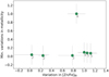 |
Fig. 7 Variation in [Zn/Fe]fit plotted against the minimum difference in metallicity for all targets. The grey numbers indicate the number of groups of components along the line of sight. |
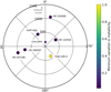 |
Fig. 8 Labelled target map, colour-coded by the minimum differences in metallicity based on our realisations. The Sun is positioned at the centre. |
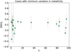 |
Fig. 9 Metallicity realisations for individual components as a function of their gas fraction for the cases with minimum difference in metallic- ity. Here we see that these cases require the gas fractions to be either very high or very low. |
4.4 Abundance patterns for the whole line of sight
Figure 10 shows the abundance patterns for full lines of sight (i.e. combining all velocity components) towards our κ Aql. The remaining targets are included in Appendix F. We performed three different linear fits for most of the targets: (1) fits to all the metals, (2) fits to only the more refractory metals (Ti II, Ni II, Cr II, Fe II, and Mn II), and (3) fits to only the more volatile metals (Mg II, Ge II, Zn II, P II, O I). We defined a limit between more refractory and more volatile elements around a value of B2X ~ 0.8. Forρ Oph A we report the fit to the only two reliable column densities. For θ1 Ori C we only included results from the fit to all metals and to the more volatile because we find the fit to the more refractory metals yields unreliable results. This could be caused by Fe-group (Ni, Cr, Fe, and Mn) over-abundance in this ISM cloud, or by peculiar Ti depletion (which is also seen in lines of sight towards other stars in this region Ritchey et al. 2023). In general, it is clear that the abundance pattern fits to all the metals are not linear, and that there is an upturn of the more volatile metals. This is likely due to the presence of a mix of gases along the lines of sight with different levels of depletion, and possibly different metallicities.
The purpose of performing linear fits to only the refractory and/or volatile elements is to show that we find that these two strategies measure different metallicities for the same lines of sight. For a given abundance pattern, fits to only the more refractory metals systematically produce lower metallicities, while fits to only the more volatile metals result in metallicities that are more similar to fits to all the metals. If low-metallicity gas exists along the line of sight, the refractory metals are the only ones sensitive to it because the volatile elements are always dominated by the omnipresent high-metallicity gas. On the other hand, the refractory elements are mostly highly depleted in the high-metallicity gas, and their abundance can instead be dominated by the low-depletion, low-metallicity gas. It is also possible to have high metallicity gas and low dust content, for example due to dust destruction. However, our approach is agnostic to metallicity because we directly measured the dust depletion of individual components, without assumptions on the metallicity. We can expect the presence of low-metallicity gas in the ISM because there is evidence of accreting low-metallicity gas, for example from high-velocity clouds (Fox & Davé 2017).
Table 8 summarises these results. In Fig. 11, we compare our results with those from De Cia et al. (2021) and Ritchey et al. (2023). We include the metallicity gradient based on H II regions from Arellano-Córdova et al. (2020).
These results confirm that using abundance patterns to calculate the metallicity of gas along full lines of sight is an approximation, and that component-by-component analyses are important for gaining a holistic measurement of the chemical enrichment in the ISM.
Results from the abundance patterns for each target along the full line of sight.
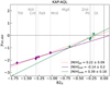 |
Fig. 10 Abundance pattern for the total line of sight towards κ Aql. |
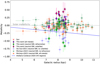 |
Fig. 11 Metallicity calculated over the full lines of sight as a function of distance from the Galactic centre for this work compared with literature results. The red diamonds are the results from the fit to abundance patterns for all metals, and the green and purple diamonds are fits to the refractory and volatile metals, respectively. We do not include the fits for ρ Oph A because of the limited data. The fit to the refractory metals for θ1 Ori C is 1.7, which we do not consider as physical, so it is excluded in this plot. |
5 Conclusions
In this work, we studied individual (groups of) components along eight lines of sight within 1.1 kpc of the Sun. We used metal patterns and the relative method to determine the amount of dust depletion [Zn/Fe]fit,i in each component. We investigated possible metallicities for these individual components by simulating 99 (4851, 156 849, 1 000 000) distributions of the total hydrogen gas between two (three, four, five) components. Our results are summarised below.
We find components with very high levels of dust depletion (up to [Zn/Fe]fit = 2.03 ± 0.03 dex or F* = 1.30) compared to the full line-of-sight analysis conducted by De Cia et al. (2021), who report a maximum depletion of 1.32 or F* = 0.53. Our study shows that full line-of-sight analyses do not capture the full range of dust depletion. This means that it is possible to have much higher levels of depletion in individual clouds compared to the full line of sight;
We find large ranges in the level of dust depletion among components along lines of sight, calculated as the difference between the minimum and maximum depletion, of up to a factor of 15 (1.19 dex);
We present a novel method of constraining the metallicities of individual gas components. We used information gained from the metals patterns – that the y-intercept is the sum of the hydrogen gas fraction and the metallicity ai = log N(H)i+ [M/H]i – with simulated log N(H)i distributions to calculate the [M/H]i for individual components. We implemented an upper metallicity limit of 0.5 dex based on results from Nepal et al. (2024). From our simulations and under this assumption, we are able to constrain metallicities for some components to within an interval of ~0.3 dex;
Our simulations indicate that, in five out of eight lines of sight, the component with the highest level of dust depletion contains the majority of the hydrogen gas, and likely has super-solar metallicity;
For the line of sight towards θ1 Ori C, we find a group of components (group 2 out of four groups) with high dust depletion, [Zn/Fe]fit,2 = 1.52 ± 0.25, the bulk of the hydrogen gas, 37% < ƒ2 < 97%, and super-solar metallicity, [M/H]2 ≥ 0.08 dex. This group of components could be attributed to the nebula itself (Price et al. 2001). Further, we find that group 4 has a low level of depletion, [Zn/Fe]fit,4 = 0.60 ± 0.21, and likely a low metallicity, at least for the case with the minimum difference in metallicity;
From our realisations, we find that the minimum variation in metallicity is <0.15 dex for all targets, with the exception of θ1 Ori C, which we find to be 1.02 dex. Although the metallicity of individual gas components cannot be strictly measured, this methodology allows us to study the minimum variations in metallicity from component to component.
With the methodology we developed in this study to constrain the metallicities of individual gas clouds in the solar neighbourhood, we are able to study the ISM in more detail and gain a better understanding of the level of chemical variation in the ISM.
Data availability
Appendices C–G are available on Zenodo at https://zenodo.org/records/14793736.
Acknowledgements
Edward B. Jenkins passed away just before the submission of this paper. Ed was one of the great fathers of UV astronomy and his scientific work on the ISM was immensely impactful and inspiring. We are grateful to have had the opportunity to work with and learn from him. His legacy will live on. Daniel E. Welty calculated the column densities for the targets θ1 Ori C, χ Oph and κ Aql. The authors acknowledge and thank him for his significant and valuable contributions to this paper. T.R.-H., A.D.C., J.-K.K., C.K. and A.V. acknowledge support by the Swiss National Science Foundation under grant 185692. This work is based on observations with the NASA/ESA Hubble Space Telescope obtained from Mikulski Archive for Space Telescopes at the Space Telescope Science Institute, which is operated by the Association of Universities for Research in Astronomy, Incorporated, under NASA contract NAS5-26555. We also make use of optical data from the European Southern Observatory, Kitt Peak National Observatory, McDonald Observatory and the Anglo-Australian Telescope. Support for programme number 16750 was provided through a grant from the STScI to Princeton University and STScI under NASA contract NAS5-26555. This research has made use of NASA’s Astrophysics Data System.
Appendix A Details of observations
Table A.1 shows the details of the HST/STIS cycle 29 observations (ID 16750) used in this work.
Observing details for HST cycle 29 programme ID 16750.
Appendix B Methodology test
We tested the methodology described in Sect. 3 by adding an extra component with known metallicity and total hydrogen column density to the line of sight towards HD 206267. This component, chosen from the SMC, helps us verify that our method can accurately recover the metallicity difference between the Milky Way and the SMC. We used data from De Cia et al. (2024) for AzV 78, who report [Zn/Fe]fit = 0.62 ± 0.12, [M/H] = −0.82 ± 0.17 and log N(H) = 21.7 ± 0.06. We chose the sight line towards HD 206267 because it has only two components with relatively low dust depletion, reducing the degeneracy between the components. This makes the hydrogen gas fraction for the SMC component fSMC = 74%.
For 5 out of the 4865 most likely realisations (i.e. metallic- ities of all components are < 0.5 dex) from this exercise, we recover a difference in metallicities of > 0.6 dex between both Milky Way clouds and the SMC (i.e. [M/H]MW1− [M/H]SMC > 0.6 dex and [M/H]MW2− [M/H]SMC > 0.6 dex). These realisations also reproduce the SMC metallicity of −0.82 ± 0.17. There is one realisation that produces a difference of 0.8 dex, and none produce a difference larger than than this. In the 0.8 dex case, the SMC metallicity is also reproduced. Figure B.1 shows the five realisations with metallicity differences > 0.6 dex in the green points and the 1 realisation that produces a difference of > 0.8 dex in purple, plotted over all of the ‘most likely’ realisations in grey (see Sect. 4.2). The metallicity of the SMC cloud is shown by the horizontal dotted black line. The gas fraction histogram in the bottom panel shows that this exercise somewhat reproduces the SMC gas fraction.
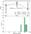 |
Fig. B.1 Results from testing of our method in Sect. 3.3, showing we reproduce the large range in metallicity between the Milky Way and the SMC for 5 out of the 4865 realisations. Top: All the ‘most likely’ realisations (in grey) and those that recover a 0.6 dex difference in metallicity between both of the Milky Way clouds and the SMC cloud (in green). Bottom: Histogram of the total hydrogen gas distributions for these realisations. |
References
- Arellano-Córdova, K. Z., Esteban, C., García-Rojas, J., & Méndez-Delgado, J. E. 2020, MNRAS, 496, 1051 [Google Scholar]
- Asplund, M., Amarsi, A. M., & Grevesse, N. 2021, A&A, 653, A141 [NASA ADS] [CrossRef] [EDP Sciences] [Google Scholar]
- Balashev, S. A., Noterdaeme, P., Rahmani, H., et al. 2017, MNRAS, 470, 2890 [CrossRef] [Google Scholar]
- Blitz, L., & Rosolowsky, E. 2006, ApJ, 650, 933 [NASA ADS] [CrossRef] [Google Scholar]
- Boissé, P., & Bergeron, J. 2019, A&A, 622, A140 [EDP Sciences] [Google Scholar]
- Brown, M. S., Alkhayat, R. B., Irving, R. E., et al. 2018, ApJ, 868, 42 [NASA ADS] [CrossRef] [Google Scholar]
- Cashman, F. H., Kulkarni, V. P., Kisielius, R., Ferland, G. J., & Bogdanovich, P. 2017, VizieR On-line Data Catalog: J/ApJS/230/8 [Google Scholar]
- Crain, R. A., Schaye, J., Bower, R. G., et al. 2015, MNRAS, 450, 1937 [NASA ADS] [CrossRef] [Google Scholar]
- De Cia, A., Ledoux, C., Mattson, L., et al. 2016, A&A, 596, A97 [NASA ADS] [CrossRef] [EDP Sciences] [Google Scholar]
- De Cia, A., Jenkins, E. B., Fox, A. J., et al. 2021, Nature, 206 [Google Scholar]
- De Cia, A., Roman-Duval, J., Konstantopoulou, C., et al. 2024, A&A, 683, A216 [NASA ADS] [CrossRef] [EDP Sciences] [Google Scholar]
- Draine, B. T. 2003, ARA&A, 41, 241 [NASA ADS] [CrossRef] [Google Scholar]
- Field, G. B. 1974, ApJ, 187, 453 [NASA ADS] [CrossRef] [Google Scholar]
- Fitzpatrick, E. L., & Spitzer, Lyman, J. 1994, ApJ, 427, 232 [NASA ADS] [CrossRef] [Google Scholar]
- Fox, A., & Davé, R. 2017, Gas Accretion onto Galaxies, Astrophysics and Space Science Library, 430 [Google Scholar]
- Fox, A. J., Richter, P., Ashley, T., et al. 2019, ApJ, 884, 53 [NASA ADS] [CrossRef] [Google Scholar]
- Jenkins, E. B. 2009, ApJ, 700, 1299 [Google Scholar]
- Jenkins, E. B., Savage, B. D., & Spitzer, L. 1986, ApJ, 301, 355 [NASA ADS] [CrossRef] [Google Scholar]
- Jenkins, E. B., & Wallerstein, G. 2017, ApJ, 838, 85 [NASA ADS] [CrossRef] [Google Scholar]
- Konstantopoulou, C., De Cia, A., Krogager, J.-K., et al. 2022, A&A, 666, A12 [NASA ADS] [CrossRef] [EDP Sciences] [Google Scholar]
- Konstantopoulou, C., De Cia, A., Krogager, J.-K., et al. 2023, A&A, 674, C1 [NASA ADS] [CrossRef] [EDP Sciences] [Google Scholar]
- Konstantopoulou, C., De Cia, A., Krogager, J.-K., et al. 2024, A&A, 691, A129 [NASA ADS] [CrossRef] [EDP Sciences] [Google Scholar]
- Krogager, J.-K. 2018, VoigtFit: Absorption line fitting for Voigt profiles, Astrophysics Source Code Library [record ascl:1811.016] [Google Scholar]
- Lallement, R., Welsh, B. Y., Vergely, J. L., Crifo, F., & Sfeir, D. 2003, A&A, 411, 447 [EDP Sciences] [Google Scholar]
- Lodders, K., Palme, H., & Gail, H. P. 2009, Solar System, Landolt-Börnstein - Group VI Astronomy and Astrophysics, 4B, 712 [CrossRef] [Google Scholar]
- Mattsson, L., De Cia, A., Andersen, A. C., & Zafar, T. 2014, MNRAS, 440, 1562 [NASA ADS] [CrossRef] [Google Scholar]
- Morton, D. C. 2003, ApJS, 149, 205 [Google Scholar]
- Nelson, D., Pillepich, A., Springel, V., et al. 2019, MNRAS, 490, 3234 [Google Scholar]
- Nepal, S., Chiappini, C., Guiglion, G., et al. 2024, A&A, 681, L8 [NASA ADS] [CrossRef] [EDP Sciences] [Google Scholar]
- Pan, K., Federman, S. R., Cunha, K., Smith, V. V., & Welty, D. E. 2004, VizieR On-line Data Catalog: J/ApJS/151/313 [Google Scholar]
- Péroux, C., Nelson, D., van de Voort, F., et al. 2020, MNRAS, 499, 2462 [CrossRef] [Google Scholar]
- Phillips, A. P., Gondhalekar, P. M., & Pettini, M. 1982, MNRAS, 200, 687 [NASA ADS] [CrossRef] [Google Scholar]
- Pillepich, A., Nelson, D., Springel, V., et al. 2019, MNRAS, 490, 3196 [Google Scholar]
- Price, R. J., Crawford, I. A., Barlow, M. J., & Howarth, I. D. 2001, MNRAS, 328, 555 [CrossRef] [Google Scholar]
- Ramburuth-Hurt, T., De Cia, A., Krogager, J. K., et al. 2023, A&A, 672 [Google Scholar]
- Richter, P. 2017, in Gas Accretion onto Galaxies, eds. A. Fox & R. Davé, Astrophysics and Space Science Library, 430, 15 [NASA ADS] [CrossRef] [Google Scholar]
- Ritchey, A. M., Jenkins, E. B., Shull, J. M., et al. 2023, ApJ, 952, 57 [NASA ADS] [CrossRef] [Google Scholar]
- Roman-Duval, J., Jenkins, E. B., Tchernyshyov, K., et al. 2021, ApJ, 910, 95 [NASA ADS] [CrossRef] [Google Scholar]
- Routly, P. M., & Spitzer, Lyman, J. 1952, ApJ, 115, 227 [NASA ADS] [CrossRef] [Google Scholar]
- Savage, B. D., & Sembach, K. R. 1996, ARA&A, 34, 279 [Google Scholar]
- Savage, B. D., Bohlin, R. C., Drake, J. F., & Budich, W. 1977, ApJ, 216, 291 [NASA ADS] [CrossRef] [Google Scholar]
- Schaye, J., Crain, R. A., Bower, R. G., et al. 2015, MNRAS, 446, 521 [Google Scholar]
- Siluk, R. S., & Silk, J. 1974, ApJ, 192, 51 [NASA ADS] [CrossRef] [Google Scholar]
- Spirko, J. A., Neiman, M. L., Oelker, A. M., & Klier, K. 2004, Surf. Sci., 572, 191 [NASA ADS] [CrossRef] [Google Scholar]
- Stancil, P. C., Schultz, D. R., Kimura, M., et al. 1999, A&AS, 140, 225 [NASA ADS] [CrossRef] [EDP Sciences] [Google Scholar]
- Valencic, L. A., Clayton, G. C., & Gordon, K. D. 2004, ApJ, 616, 912 [NASA ADS] [CrossRef] [Google Scholar]
- Velichko, A., De Cia, A., Konstantopoulou, C., et al. 2024, A&A, 685, A103 [NASA ADS] [CrossRef] [EDP Sciences] [Google Scholar]
- Welty, D. E., & Crowther, P. A. 2010, MNRAS, 404, 1321 [NASA ADS] [Google Scholar]
- Welty, D. E., & Hobbs, L. M. 2001, ApJS, 133, 345 [NASA ADS] [CrossRef] [Google Scholar]
- Welty, D. E., Hobbs, L. M., & York, D. G. 1991, ApJS, 75, 425 [NASA ADS] [CrossRef] [Google Scholar]
- Welty, D. E., Hobbs, L. M., & Morton, D. C. 2003, ApJS, 147, 61 [NASA ADS] [CrossRef] [Google Scholar]
- Welty, D. E., Sonnentrucker, P., Snow, T. P., & York, D. G. 2020, ApJ, 897, 36 [Google Scholar]
- Zucker, C., Goodman, A. A., Alves, J., et al. 2022, Nature, 601, 334 [NASA ADS] [CrossRef] [Google Scholar]
All Tables
Target information with distances from the Galactic centre calculated using Gaia DR3.
Rest wavelengths, oscillator strengths and their reference for the transitions considered in this work.
Five sight lines where the component with the highest depletion also contains the majority of the hydrogen gas.
Metallicities and corresponding gas fractions for the cases with the minimum difference in metallicity.
Minimum and maximum metallicities and their respective ɀ-test significance for the minimum-difference realisation.
Results from the abundance patterns for each target along the full line of sight.
All Figures
|
Fig. 1 Distributions of total hydrogen gas fractions that we used to infer the metallicities of individual components. From top to bottom: distributions for two to five components, respectively. The histograms for four and five components are plotted in log-scale for visual clarity. |
| In the text | |
|
Fig. 2 Metal patterns for grouped components towards χ Oph. This line of sight has the highest dust depletion of our sample, with [Zn/Fe]fit,3 = 2.03 ± 0.13 dex. |
| In the text | |
|
Fig. 3 Depletion factors for individual components along each line of sight (green points). The [Zn/Fe]fit values for the entire line of sight are plotted as red diamonds. |
| In the text | |
|
Fig. 4 Velocity-depletion plot for groups of components. |
| In the text | |
|
Fig. 5 Simulation realisations for the most likely cases (where the metallicities for all groups are ≤0.5 dex) for χ Oph. The solid grey horizontal line in the top panel represents the metallicity along the whole line of sight, taking into account all of the metals. The points with black edges connected by the black line highlight the case with the minimum differences in metallicity. The grey-shaded region above 0.5 dex shows the upper bound criteria for the metallicities. The colours of the points correspond to the gas fraction of the first group N(H1) for each realisation (i.e. approximately 1% ≤ f1 ≤ 45%), as indicated in the colour bar. The histograms in the following panels are the total hydrogen gas fractions, fi, for the most likely cases. We include the level of dust depletion [Zn/Fe]fit,i in the legends. |
| In the text | |
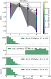 |
Fig. 6 Same as Fig. 5, but for θ1 Ori C. |
| In the text | |
|
Fig. 7 Variation in [Zn/Fe]fit plotted against the minimum difference in metallicity for all targets. The grey numbers indicate the number of groups of components along the line of sight. |
| In the text | |
|
Fig. 8 Labelled target map, colour-coded by the minimum differences in metallicity based on our realisations. The Sun is positioned at the centre. |
| In the text | |
|
Fig. 9 Metallicity realisations for individual components as a function of their gas fraction for the cases with minimum difference in metallic- ity. Here we see that these cases require the gas fractions to be either very high or very low. |
| In the text | |
|
Fig. 10 Abundance pattern for the total line of sight towards κ Aql. |
| In the text | |
|
Fig. 11 Metallicity calculated over the full lines of sight as a function of distance from the Galactic centre for this work compared with literature results. The red diamonds are the results from the fit to abundance patterns for all metals, and the green and purple diamonds are fits to the refractory and volatile metals, respectively. We do not include the fits for ρ Oph A because of the limited data. The fit to the refractory metals for θ1 Ori C is 1.7, which we do not consider as physical, so it is excluded in this plot. |
| In the text | |
|
Fig. B.1 Results from testing of our method in Sect. 3.3, showing we reproduce the large range in metallicity between the Milky Way and the SMC for 5 out of the 4865 realisations. Top: All the ‘most likely’ realisations (in grey) and those that recover a 0.6 dex difference in metallicity between both of the Milky Way clouds and the SMC cloud (in green). Bottom: Histogram of the total hydrogen gas distributions for these realisations. |
| In the text | |
Current usage metrics show cumulative count of Article Views (full-text article views including HTML views, PDF and ePub downloads, according to the available data) and Abstracts Views on Vision4Press platform.
Data correspond to usage on the plateform after 2015. The current usage metrics is available 48-96 hours after online publication and is updated daily on week days.
Initial download of the metrics may take a while.