| Issue |
A&A
Volume 695, March 2025
|
|
|---|---|---|
| Article Number | A8 | |
| Number of page(s) | 12 | |
| Section | Extragalactic astronomy | |
| DOI | https://doi.org/10.1051/0004-6361/202449208 | |
| Published online | 26 February 2025 | |
A synthetic population of ultra-luminous X-ray sources
Optical–X-ray correlation
1
Centre for Astro-Particle Physics (CAPP) and Department of Physics, University of Johannesburg, PO Box 524 Auckland Park 2006, South Africa
2
Department of Physics, The George Washington University, Washington, DC 20052, USA
3
National Institute for Theoretical and Computational Sciences (NITheCS), Private Bag X1, Matieland, South Africa
4
U.S. Naval Research Laboratory, Code 7653, 4555 Overlook Ave. SW, Washington, DC 20375-5352, USA
⋆ Corresponding authors; lnyadzani@uj.ac.za, srazzaque@uj.ac.za, justin.d.finke.civ@us.navy.mil
Received:
11
January
2024
Accepted:
21
January
2025
This paper presents an analysis of the predicted optical-to-X-ray spectral index (αox) within the context of ultra-luminous X-ray sources (ULXs) associated with stellar-mass black holes (BHs) and neutron stars (NSs). We used the population synthesis code COSMIC to simulate the evolution of binary systems and investigate the relationship between ultraviolet (UV) and X-ray emission during the ULX phase, namely the αox relation. Furthermore, we investigated the impact of metallicity on αox values. Notably, it predicts a significant anti-correlation between αox and UV luminosity (LUV), consistent with observations. The slope of this relationship varies with metallicity for black hole ULXs (BH-ULXs). The neutron star ULX (NS-ULX) population shows a relatively consistent slope around −0.33 across metallicities, with minor variations. The number of ULXs decreases with increasing metallicity, consistent with observational data. The X-ray luminosity function (XLF) shows a slight variation in its slope with metallicity, exhibiting a relative excess of high-luminosity ULXs at lower metallicities. The inclusion of the beaming effect in the analysis shows a significant impact on the XLF and αox, particularly at high accretion rates, where the emission is focused into narrower cones. We found that UV emission in ULXs is predominantly disc-dominated, which is the likely origin of the αox relation, with the percentage of disc-dominated ULXs increasing as metallicity rises.
Key words: binaries: general
© The Authors 2025
 Open Access article, published by EDP Sciences, under the terms of the Creative Commons Attribution License (https://creativecommons.org/licenses/by/4.0), which permits unrestricted use, distribution, and reproduction in any medium, provided the original work is properly cited.
This article is published in open access under the Subscribe to Open model. Subscribe to A&A to support open access publication.
1. Introduction
Ultra-luminous X-ray sources (ULXs) are extragalactic point-like sources that exhibit extraordinarily high luminosities in the X-ray (LX > 1039 erg/s), exceeding the Eddington luminosity for black holes (BHs) of mass ≈10 M⊙. The first ULXs were discovered using the Einstein Observatory, designed to obtain images of distant galaxies (for a review, see Fabbiano 1989). Early X-ray surveys revealed a considerable quantity of these sources. Fabbiano (1989) identified 16 sources with X-ray luminosities LX > 1039 erg/s. To date, over 1800 ULXs have been identified, increasing our knowledge and understanding of ULX sources (Kaaret et al. 2017; Walton et al. 2022; King et al. 2023).
Since their discovery, the debate over what powers these systems has been a continuous topic of both theory and observation. Theoretically, there are three possibilities as to how these systems reach such high luminosities: (1) accretion by intermediate mass black holes (IMBH), 102 to 105 M⊙, (Colbert & Mushotzky 1999): this increases the mass of the BH, and the system accretes at sub-Eddington rate; (2) beamed emission from a stellar-mass BH or neutron star (NS) (Georganopoulos et al. 2002): this avoids super-Eddington accretion and keeps the mass of the compact object below 100 M⊙; and (3) super-Eddington accretion (e.g. Begelman 2001; Finke & Böttcher 2007; Sądowski & Narayan 2015): accretion onto stellar mass BHs or NSs emitting with a super-Eddington luminosity. We note that a system can simultaneously be beamed and supercritical. Observations have shown evidence for IMBHs (Lasota et al. 2011; Mezcua et al. 2013), stellar mass BHs (Middleton et al. 2013), and pulsations detected in a few systems indicate the presence of an NS (Bachetti et al. 2014; Fürst et al. 2016) as the primary object in these systems. It has been suggested that ULXs could be the progenitors of compact object mergers detected by LIGO (Inoue et al. 2016; Finke & Razzaque 2017; Mondal et al. 2020).
The debate on ULXs centres around the mass of the compact objects and their accretion rate. While X-ray data have been instrumental in our understanding of ULXs, they have limitations. They often do not provide information about the companion of the compact object. Identifying the companion can offer valuable insights into the masses of these binary systems. An example of the significance of this approach can be found in the confirmation of the existence of Cygnus X-1, the first known Galactic BH (Murdin & Webster 1971). ULXs also emit radiation in other wavelengths, including the ultraviolet (UV) and optical bands (Gladstone et al. 2013).
Previous observational studies have provided valuable insights into the connection between X-ray and UV radiation in ULXs, suggesting a common origin or interconnected emission mechanisms. Sonbas et al. (2019) investigated the relationship between the X-ray and UV wavebands in several ULXs with known optical counterparts by comparing the ratio of flux densities and by utilising the spectral optical–X-ray index, αox. Their analysis reveals a significant anti-correlation between αox and the UV luminosity at 2500 Å (L2500 Å). However, due to the complexity of ULX systems and the limitations of observational data, it is challenging to fully explore and understand the correlation between X-ray and UV radiation based only on observations. Therefore, simulated studies that follow the evolution of binary systems and model the emission processes to provide detailed insights into the spectral behaviour are essential. Simulated studies enable us to disentangle the complex interplay of physical mechanisms in astrophysical sources, allowing us to explore a wide parameter space and investigate various emission scenarios. By employing a population synthesis code, we simulated a range of ULX scenarios and systematically studied the spectral correlation between X-ray and UV radiation.
In this work, we used the population synthesis code COSMIC (Breivik et al. 2020) to simulate the evolution of binary systems and study the relationship between the UV and X-ray emission of ULXs. We explored the effects of metallicity on the synthetic population of ULXs and the αox relation for BH-ULXs and NS-ULXs and compared them with observational data. The layout of the paper is as follows: in Sect. 2, we discuss our COSMIC simulation set-up; the UV- and X-ray-emission models are discussed in Sect. 3; and in Sect. 4 we present and discuss our results. We summarise and conclude our study in Sect. 5.
2. Synthetic binary population
To study the correlation between X-ray and UV radiation in ULXs, we employed the COSMIC (Breivik et al. 2020) binary population synthesis code. COSMIC combines theoretical models of stellar evolution, binary interactions, and compact object mergers to simulate the formation and evolution of binary systems. We modeled the evolution of binaries starting from the zero-age main sequence (ZAMS) until the formation of the X-ray binary systems.
In our simulations, we drew the primary (most massive) ZAMS mass, M1, from a Kroupa initial mass function (IMF; Kroupa et al. 1993). This IMF is given by dN/dM1 ∝ M1−α, with α = 1.3 for 0.08 M⊙ < M1 ≤ 0.5 M⊙; α = 2.2 for 0.5 M⊙ < M1 ≤ 1 M⊙; and α = 2.7 for M1 > 1.0 M⊙. The ZAMS mass of the secondary star, M2 (ranging from 0.5 M⊙ to 150 M⊙), was drawn from a flat distribution of the binary mass ratio q = M2/M1 within the range of [0.1, 1.0]. The orbital period (P) was drawn from a distribution of f(log10P/d)≈(log10P/d)−0.55, with log10P/d ranging from 0.15 to 5.5, and the eccentricity (e) was drawn from a distribution that followed f(e)≈e−0.42 within the interval of [0.0, 0.9] (Sana et al. 2013).
In our study, we simulated 2 × 10⁶ binary systems with varying metallicities, ranging from 0.5% of the solar metallicity (Z⊙) to 1.5 Z⊙. The precise value of Z⊙ remains uncertain (Vagnozzi et al. 2017). We adopted Z⊙ = 0.02 as the benchmark value for consistency with previous studies (e.g. Mondal et al. 2020). Additionally, we set the binary fraction to be 100% for a primary mass greater than 10 M⊙ (Sana et al. 2013). The configurations in our standard COSMIC model parameters are as follows.
-
Common envelope (CE) phase: CE efficiency of αCE = 1, we follow the pessimistic scenario by letting stars without a core-envelope boundary to automatically lead to merger during the CE phase (Belczynski et al. 2007).
-
Supernova model: to estimate the mass of the final compact object after the supernova explosion, we followed the rapid supernova model (Fryer et al. 2012).
-
Accretion: studies using simulations have demonstrated that mass accretion onto a compact object can exceed the Eddington limit (McKinney et al. 2014). It is now considered possible for super-Eddington accretion to occur in X-ray binaries with both BHs and NSs as compact objects (Van Den Eijnden et al. 2019; Vasilopoulos et al. 2020). Therefore, we allowed super-Eddington accretion to reach values of up to 1000 times the Eddington limit.
-
Critical mass ratios (qc): qc, is the mass ratio between the donor and accretor at the beginning of Roche-lobe overflow (RLOF). It is used to determine whether a system will experience a CE phase or continue with stable mass transfer (MT) based on the mass ratio of the components at the beginning of RLOF. Mass transfer through RLOF is only allowed for a thermal timescale if the mass ratio at the beginning of RLOF is below the qc. If the mass ratio ≥qc, the mass transfer occurs on a dynamic timescale, resulting in the initiation of the CE phase. To determine qc, we followed the treatment in Sect. 5.1 of Belczynski et al. (2008).
We sampled a population of main-sequence binary stars that evolved from the ZAMS until the formation of X-ray binary systems. Our ULX population is selected based on the value of X-ray luminosity, LX > 1039 erg/s. In the next section, we discuss how our X-ray and UV luminosities are calculated.
3. Emission from the accretion disc and donor star
3.1. Total X-ray emission
The X-ray emission from ULXs primarily originates from the accretion processes onto the compact objects: either stellar-mass BHs or NSs. In these systems, a massive donor star transfers mass to the compact object through RLOF or wind accretion. The high luminosities observed in ULXs, exceeding the Eddington limit for typical stellar-mass BHs, suggest the presence of highly efficient accretion processes. Accretion models play a crucial role in our understanding of the X-ray emission from ULXs and require the careful consideration of their physical parameters and radiative processes.
In a compact binary system, mass is transferred from one star to another. This process leads to the creation of an accretion disc. We calculate an isotropic bolometric X-ray luminosity (LX, iso) from accretion as (Shakura & Sunyaev 1973; Poutanen et al. 2007)
![$$ \begin{aligned} L_{\rm X,iso} = {\left\{ \begin{array}{ll} L_{\rm Edd}[1+\ln \dot{m}]&\mathrm{if}\; \dot{m} > 1 \\ \eta \dot{M}c^2&\mathrm{if}\; \dot{m} \le 1. \end{array}\right.} \end{aligned} $$](/articles/aa/full_html/2025/03/aa49208-24/aa49208-24-eq1.gif)
Here, Ṁ is the mass-accretion rate, c is the speed of light, ṁ is the ratio Ṁ/ṀEdd between the mass accretion rate and the Eddington accretion rate ṀEdd = 12LEdd/c2, LEdd is the Eddington luminosity of a star or compact object with mass M given by
η is the accretion efficiency defined as

for NSs, and

for BHs, where G is Newton’s gravitational constant. The function E(R) is given by
![$$ \begin{aligned} E(R) = \frac{R^2-2\frac{GM}{c^2}R+a\frac{GM}{c^2}\left(\frac{GM}{c^2}R\right)^{1/2}}{R\left[R^2-3\frac{GM}{c^2}R+2a\frac{GM}{c^2} \left(\frac{GM}{c^2}R\right)^{1/2}\right]^{1/2}}, \end{aligned} $$](/articles/aa/full_html/2025/03/aa49208-24/aa49208-24-eq5.gif)
where a is the BH spin and RISO is the radius of the innermost stable orbit,
![$$ \begin{aligned}&R_{\mathrm{ISO}} = \frac{R_{\mathrm{Sch}}}{2} \left(3 + Z_2 - \left[(3 - Z_1) (3 + Z_1 + 2Z_2)\right]^{1/2}\right),\end{aligned} $$](/articles/aa/full_html/2025/03/aa49208-24/aa49208-24-eq6.gif)
![$$ \begin{aligned}&Z_1 = 1 + \left(1 - \frac{4a^2}{R_{\mathrm{Sch}}^2}\right)^{1/3} \left[\left(1 + \frac{2a}{R_{\mathrm{Sch}}}\right)^{1/3} + \left(1 - \frac{2a}{R_{\mathrm{Sch}}}\right)^{1/3}\right],\end{aligned} $$](/articles/aa/full_html/2025/03/aa49208-24/aa49208-24-eq7.gif)
where RSch = 2GM/c2 is the Schwarzschild radius (Brown et al. 2000).
When the accretion rate is high, the luminosity can be focused into narrow cones, resulting in greater observed luminosity compared to the isotropic emission. This phenomenon is referred to as ‘beaming’. In order to explore the potential impact of the beaming factor, we followed King (2009) to calculate the beaming factor (b), which is given by
The beamed X-ray luminosity is then given by

where LX, iso is the X-ray luminosity in Eq. (1).
3.2. ULX spectrum
In addition to their intense X-ray emission, ULXs emit in the optical and UV. The presence of UV emission in conjunction with X-ray radiation opens a window to understanding the broader radiative processes at play in these enigmatic systems. This dual emission may hold clues to the intricate interconnections between the various components of the accretion process, the accretion disc, companion stars, and the surrounding environment. To study ULXs in both the UV and X-ray bands, it is essential to consider contributions from both the accretion disc and the stellar companion. The X-ray emission primarily originates from the accretion disc, whereas the UV emission has two components: one from the disc and another from the stellar companion. In this section, we describe the models utilised in our calculations.
3.2.1. Accretion disc
Ultra-luminous-X-ray-source spectral modelling has been a focus in several studies using models such as DISKBB (Mitsuda et al. 1984) and DISKIR (Gierliński et al. 2008, 2009). These models often imply the presence of high-mass black holes in the ULX systems, which are not the focus of this study. Vinokurov et al. (2013) proposed a physically motivated model by examining the spectral energy distribution (SED) of supercritical accretion discs (SCADs) and applied this model to fit the observed SEDs of five ULXs.
According to the SCAD model, the accretion discs become thick and develop a strong wind, forming a wind funnel above the disc at distances shorter than the spherisation radius, with a temperature dependence given by T ∝ r−1/2. The disc’s luminosity in this region is approximated by Lbol ≈ LEdd ln (ṁ). Outside the spherisation radius, the disc remains thin, and its total luminosity equals the Eddington luminosity, LEdd. The thin disc heats the wind from below, and from the inner side of the funnel the wind is heated by the supercritical disc (see Fig. 2 of Vinokurov et al. 2013).
When applied to ULX spectra, the SCAD model suggests stellar-mass BHs as the compact object, whereas the DISKIR model often yields much higher BH masses, suggesting IMBHs. The SCAD model accounts for the high-energy curvature observed in ULX spectra and the presence of outflows without invoking IMBHs. It explains the observed luminosities and spectral features using stellar-mass BHs undergoing supercritical accretion, which is consistent with the lack of a large population of IMBHs observationally. Since all our simulated ULXs have either stellar-mass BHs or NSs as the compact objects, we used the SCAD model to describe the supercritical accretion discs in our simulated ULX population. The temperature of the disc in this model is given by
![$$ \begin{aligned} T(r) = T_{\rm in} {\left\{ \begin{array}{ll} (r \sin \theta _{f})^{-1/2},&1 \le r \le r_{\rm sp} \\ \Big [\frac{f_{\rm out}}{\sin \theta _{f}} (1 + \ln \dot{m})\Big ]^{1/4}r^{-1/2},&r_{\rm sp} \le r \le r_{\rm ph} \end{array}\right.} , \end{aligned} $$](/articles/aa/full_html/2025/03/aa49208-24/aa49208-24-eq11.gif)
where Tin4 = LEddsin(θf)/(4πσRin2), Rin = 3RSch = 6GM/c2, M is the compact object mass, θf is the funnel angle, σ is the Stefan-Boltzmann constant, fout is the fraction of bolometric flux thermalised in the disc, and r = R/Rin is the radius of the accretion disc. Here, rsp = Ṁ/ṀEdd is the spherisation radius, and  is the photospheric radius, where κ is the opacity (κ ≈ κes = 0.34 cm2/g for fully ionised gas) and vw = 1000 km s−1 is the wind velocity. With our COSMIC data, this leaves only fout and θf as free parameters in this model. The effect of these two free parameters is discussed in the results section. The luminosity, at a given frequency ν and radius r within a thickness of dr of the disc, can be expressed as

where
is the Planck function describing black-body radiation at a given temperature, T, and a given frequency, ν. Here, h is the Planck constant and k is the Boltzmann constant. Therefore, the total luminosity as a function of frequency, considering the temperature gradient, is
3.2.2. Stellar companion
Another component of the ULX spectrum is the companion star, which mainly contributes to the UV band. Observations have indicated that the most likely donor stars are massive and hot OB-type stars, which can contribute significantly to the UV emission (Liu et al. 2004; Roberts et al. 2008; Gladstone et al. 2013). Other studies have found evolved red super-giant companions (Heida et al. 2015, 2019). This emission can also be attributed to the high-energy radiation absorbed and re-emitted by the donor star’s surface (Middleton et al. 2015). The UV luminosity from a companion star of radius (R⋆) and effective temperature (T⋆) is obtained by
where we use λ = c/ν = 2500 Å. The UV contribution from the disc (LUV, disk) is obtained from Eq. (14) at λ = 2500 Å. Then, the total UV emission from the ULX is given by

4. Results and discussion
Our study aims to simulate a population of ULXs, investigate their properties, and compare them to the observed population. In this section we show our results and compare them to the observational data where available.
4.1. Number of ULXs
Various studies have explored the relationship between the number of ULXs, star formation rate (SFR), and metallicity. Using the population synthesis code StarTrack, Wiktorowicz et al. (2017) simulated a robust correlation between the number of ULXs and the SFR history. Meanwhile, Mondal et al. (2020), also using StarTrack, found an increase in the number of ULXs with decreasing metallicity in their simulations, specifically in the context of stars born at the same time (i.e. a single burst). In an X-ray survey of a sample of 66 galaxies, Mapelli et al. (2011) found that there is no significant direct correlation between the number of ULXs (NULX) and metallicity. However, when normalising the number of ULXs by the SFR, (NULX/SFR), a marginally significant anti-correlation with metallicity is observed. This indicates that lower metallicity environments produce more ULXs per unit of star formation compared to higher metallicity environments. These studies show that metallicity has some influence on the efficiency of ULX formation, but this effect is secondary to the influence of SFR. Mapelli et al. (2011) also found the power-law index of  for NULX/SFR, where the number of ULX is normalised by the SFR and
  for NULX as a function of metallicity.
In Fig. 1, we show NULX as a function of metallicity for our simulations. We note that we define NULX from our synthetic population at the end of the ULX phase. The time evolution of ULX population properties will be the focus of future studies. The total number of ULXs, as well as the sub-populations of BH-ULXs and NS-ULXs, show a declining trend with increasing metallicity. The slope for BH-ULXs is steeper (α = 0.21 ± 0.02) compared to the total ULX population (α = 0.16 ± 0.01) and NS-ULXs (α = 0.09 ± 0.01). At higher metallicities, the populations of NS-ULXs and BH-ULXs become comparable. The steeper decline for BH-ULXs indicates that the formation of BH-ULXs is more sensitive to metallicity compared to NS-ULXs. The shallower slope for NS-ULXs suggests that while metallicity does affect their formation, it is not as critical as for BH-ULXs. This aligns with the theoretical understanding that massive metal-poor stars are more likely to form massive BHs through direct collapse (Heger et al. 2003). Our power-law index of α = 0.16 ± 0.01 for the combined population of BH- and NS-ULXs is consistent with the slope from Mapelli et al. (2011).
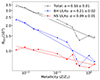 |
Fig. 1. Number of ULXs formed in our simulation (NULX) as a function of metallicity. The y-axis indicates the number of ULXs derived from the simulations, with emphasis placed on the trend’s shape rather than the absolute values. The solid lines represent fits to the simulated data, with the corresponding slopes mentioned in the legend. |
The parameters fout and θf in Eq. (11) play a crucial role in shaping the UV and X-ray emission characteristics of ULXs. A higher fraction of the bolometric flux thermalised in the disc (i.e. larger fout) results in stronger UV emission. Conversely, for any observer viewing the system down the funnel formed by the disc combination, smaller θf angles will result in enhanced X-ray emission by directing more of the X-ray emission into the increasingly narrow funnel. For our simulated populations, we set fout to the average value derived from the systems analysed in Vinokurov et al. (2013), adopting fout = 0.03. A detailed discussion of the impact of varying fout on our results can be found in Sect. 4.3. This value of fout ensures that a small but significant fraction of the bolometric flux is thermalised in the accretion disc, contributing to UV emission. Given the high accretion rates typical of ULXs, this thermalisation fraction effectively reproduces the observed emission without overestimating the flux.
We studied our population with θf set to 45° and treat this as a non-beamed population (see Sect. 4.2). It should be noted that θf = 45° was selected as a standard, intermediate value within the allowed range of 0° −90° for exploratory purposes and does not imply any inherent physical property of the system. In Sect. 4.3.1, we calculate θf from the accretion rate using the beaming model by King (2009) and compare the two scenarios.
4.2. Results with constant θf
4.2.1. X-ray luminosity function
One approach to studying the ULX population involves studying their X-ray luminosity function. Figure 2 shows the cumulative XLF of the simulated ULX population at 40% of Z⊙ in the 0.2−12 keV band. We fit this population with a function,
![$$ \begin{aligned} N({>}L_{\rm X}) = C L_{\rm X}^{-\alpha }\exp {[-(L_{\rm X}/L_s)^{\beta }]}, \end{aligned} $$](/articles/aa/full_html/2025/03/aa49208-24/aa49208-24-eq20.gif)
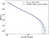 |
Fig. 2. Cumulative XLF of the simulated ULX population at 40% Z⊙ in the 0.2−12 keV band. |
and obtained power-law index α = 1.99 ± 0.02, β = 3.92 ± 3.70, and Ls = (43.7 ± 9.94)×1039 erg s−1 at this metallicity. However, the power-law index changes with metallicity. The XLF for a high-metallicity population is steeper than a low-metallicity population; it ranges from α = 1.77 ± 0.01 at 0.05 Z⊙ to 2.15 ± 0.38 at 1.5 Z⊙, showing a relative excess of high-luminosity ULXs at lower metallicities (see Table 1). Similarly, Lehmer et al. (2021) observed an increasing number of luminous sources with declining metallicity, indicating that low-metallicity environments have more high-luminosity high-mass X-ray binary (HMXB) sources.
XLF fit parameters.
4.2.2. Optical–X-ray spectral index (αox)
The X-ray-to-UV ratio is described as the interband spectral index (Tananbaum et al. 1979),
where both Lν, UV and Lν, X are expressed as monochromatic luminosities (in units of erg/s/Hz) defined at νUV = 1.2 × 10¹⁵ Hz (2500 Å) and νX = 4.8 × 10¹⁷ Hz (2 keV), respectively, following the work of Sonbas et al. (2019), who found an anti-correlation between αox and Lν,UV in observational data. In the context of the SCAD model, discussed in Sect. 3.2.1, such a relationship is expected, where the UV luminosity is dominated by emission from the funnel and depends on the accretion rate (ṁ), while the X-ray luminosity is dominated by emission from the inner accretion disc and does not depend on ṁ (see Fig. 3 in Vinokurov et al. 2013). Both the components depend on the mass of the primary in the same way. Systems with greater ṁ have greater UV luminosity but the same X-ray luminosity (for a given primary mass M). So, as ṁ increases, Lν,UV also increases, and the ratio  decreases. This leads to the anti-correlation between αox and Lν,UV. The diversity of this relation, however, depends on various factors such as the metallicity of the systems, the accretion disc’s wind velocity, the fraction of flux thermalisation in the disc, and so on. We present those results here.
Figure 3 presents the assumed SEDs for three BH-ULXs and three NS-ULXs generated from our simulations (see Fig. 3 of Vinokurov et al. 2013). The spectra are calculated at a distance of 3 Mpc using Eq. (14) without the contribution from the stellar companion. The figure also includes the key parameters for each system: M and ṁ. In Fig. A.11, we show the effect of varying ṁ for a constant M, where it is evident that the 2 keV X-ray flux is independent of ṁ, a crucial point made above for the αox and Lν,UV anti-correlation. Other studies have shown that the ULX wind velocity can be as high as 0.1c − 0.3c (Pinto & Walton 2023; Pinto et al. 2020; Kosec et al. 2018). Increasing the wind velocity from 1000 km s−1 to 60 000 km s−1 (0.2c) leads to a reduction in flux at lower frequencies and the disappearance of the UV shoulder. However, the X-ray emission at higher frequencies is unaffected by the change in wind velocity (see Fig. A.2). This results in more positive αox values and a steeper αox − Lν,UV relation (see Fig. A.4).
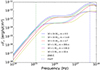 |
Fig. 3. Spectra of three BH-ULX and three NS-ULX systems from our simulation, showing the mass of the compact object (M) and the ratio ṁ = Ṁ/ṀEdd. Flux is calculated for all systems located at 3 Mpc, and for all curves fout = 0.03 and θf = 45°. |
Figure 4 shows the index αox, defined in Eq. (18), as a function of UV luminosity, combining the accretion disc and the companion star, at different metallicities (2.5%, 20%, and 40% of solar metallicity from top to bottom) of our simulated ULX population. We fit the BH- and NS-ULX simulated populations together and separately with the function
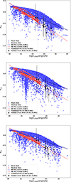 |
Fig. 4. αox index as function of Lν,UV (2500 Å) luminosity for our simulated ULX population (BH or NS primaries). The best fit to αox − Lν,UV simulated data in our population (black solid line) and observed ULXs data in Sonbas et al. (2019) (black points) are also shown. The top, middle, and bottom panels correspond to metallicities of 0.025 Z⊙, 0.20 Z⊙, and 0.40 Z⊙, respectively. We also show the αox − Lν,UV fits for the BH-ULX and NS-ULX systems separately. |

where the slope m and intercept C are free parameters. The slopes from these fits are shown in Table 2.
Slope (m) of αox versus Lν, UV.
The results presented in Table 2 reveal that the slope m of the αox − Lν,UV relation varies with metallicity and across different ULX populations. For BH-ULXs, the slope becomes less negative as metallicity increases, indicating that higher metallicities reduce the sensitivity of the X-ray to UV spectral index to UV luminosity. In contrast, NS-ULXs exhibit a relatively stable slope around −0.33 across all metallicities. This consistency implies that the SED of NS-ULXs is less affected by changes in metallicity compared to BH-ULXs. The combined population shows a similar trend to BH-ULXs, with the slope decreasing slightly with increasing metallicity. Combined slopes are closer to the BH-ULX slopes, indicating that BH-ULXs may play a slightly more dominant role in determining the overall behaviour. This is in line with the simulated BH-ULXs outnumbering the NS-ULXs in our simulated populations, as evident from Fig. 1.
Also shown in Fig. 4 are the observational data from Sonbas et al. (2019). We note that the αox values for the observed ULXs are described better by the BH-ULX systems with fout = 0.03, except, possibly, for two cases that can be explained by NS-ULX systems. The metallicities of the host galaxies of the ULXs listed in Sonbas et al. (2019) are between 0.10 Z⊙ and 0.36 Z⊙, with an average metallicity of 0.22 Z⊙. This is approximately the value corresponding to the middle panel of Fig. 4.
Figure 4 shows that most of the NS-ULX systems in our simulation are in the lower range of UV luminosities compared to the data points from Sonbas et al. (2019) with fout = 0.03. The range of Lν, UV is affected by the choice of fout. Increasing the fout value leads to high Lν, UV (see Sect. 4.3). This suggests a potential observational bias, where the observed sample might preferentially include ULXs with higher UV fluxes. This bias could occur because systems with lower UV fluxes are harder to detect and may be under-represented in the observational sample, leading to a steeper observed slope. Furthermore, our synthetic population includes systems with higher UV luminosities not present in the observational data, indicating that our simulations predict a broader range of UV luminosity for ULX systems.
4.2.3. Disc versus stellar-companion contribution to UV emission
We calculated UV emission both from the accretion disc and the stellar companion star. We find that a higher percentage of ULX systems are dominated by the disc component in the UV, which is consistent with observational studies (Tao et al. 2012). The percentage of disc-dominated ULXs increases with metallicity, starting from 77% at the lowest metallicity simulated (0.005 Z⊙) to 93% at the highest metallicity simulated (1.5 Z⊙). The percentages of ULXs with disc-dominated UV emission in Fig. 4 are 85%, 82%, and 86% from the top to the bottom panel, respectively. We also find that the majority of the NS-ULXs are dominated by the disc in the UV, leaving the slope of the companion-dominated UV systems being close to that of the BH-ULXs. We note that the companion stars that do dominate the total UV emission are primarily OB-type stars with very high surface temperatures (from 10 000 K to 50 000 K).
Figure 5 shows the αox − Lν,UV relation at 0.2 Z⊙. We note here that this is specifically for the binaries with LUV dominated by the companion. The donor-dominated BH-ULX systems display a stronger dependence on metallicity, while NS-ULX systems remain relatively unaffected by changes in metallicity (see Table 3).
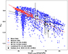 |
Fig. 5. αox for donor-star-dominated UV emission for ULX systems as a function of UV (2500 Å) luminosity for our simulated ULX population (BH or NS primaries). The best fit to αox − Lν,UV simulated data in our population (black solid) at 0.2 Z⊙ and that for observed ULXs in Sonbas et al. (2019) (black points) are also shown. |
Slope (m) of αox versus donor-dominated Lν, UV.
4.3. Impact of free parameters fout and θf on αox
In this model, the key free parameters, fout and θf, play crucial roles in shaping the reprocessing of disc radiation and the observed spectra. The parameter fout was determined by the average value in systems explored by Vinokurov et al. (2013). In reality, every system will have a different value of fout. Unfortunately, we do not have a way to determine the value of fout for each system; however, we can study the effect of varying this parameter in our population properties.
The UV emission is highly sensitive to the value of fout; higher values result in greater UV contribution (see the SED in Fig. A.3). Increasing fout makes the values of αox more negative and the slope of αox − Lν, UV relation becomes closer to that of Sonbas et al. (2019) for the combined population (see Fig. A.5). With fout = 0.2, the majority of the observed (Sonbas et al. 2019) ULXs can be explained by both NS-ULXs and BH-ULXs from our simulations.
From Fig. 3, it can be observed that the frequency corresponding to 2500 Å does not lie within the flat part of the UV and optical SED for those systems. The wind temperature scales as  , and decreasing fout shifts the flat portion of the spectrum towards higher frequencies (or, equivalently, shorter wavelengths). Hence, to place 2500 Å within the flat part of the spectrum, fout must be decreased further.
The parameter θf primarily influences the X-ray emission, making αox values more positive with decreasing θf, though it has a negligible impact on the slope of the αox − Lν,UV relation for a fixed fout. Decreasing the funnel angle from 45° to 5° represents a tenfold increase in luminosity. With θf = 45°, the most luminous BH-ULX and NS-ULX at the lowest metallicity have luminosities of LX = 1.4 × 1041 erg s−1 and LX = 5.4 × 1039 erg s−1, respectively, while the most luminous systems have LX = 4.2 × 1040 erg s−1 and LX = 5.5 × 1039 erg s−1 at the highest metallicity simulated. To fully explore the effects of varying θf, we calculated the funnel angle θf based on the accretion rate using the model proposed by King (2009) in Sect. 4.3.1.
4.3.1. Results with beaming and comparative analysis
In the initial phase of our study, we assumed a fixed funnel angle of θf = 45°, allowing us to explore the fundamental properties of ULXs and their X-ray luminosity under this assumption. However, this assumption does not fully capture the dynamic nature of accretion processes, particularly at high accretion rates where the emission is expected to be highly beamed (King et al. 2001). According to King et al. (2001) and later refined by King (2009), the funnel angle θf varies with the accretion rate ṁ according to Eq. (9). When the accretion rate is high, the luminosity is focused into narrower cones, significantly enhancing the observed luminosity. The beaming factor b is defined as
where Ω is the solid angle of emission. For a conical beam with an opening angle of θf, the solid angle is given by
We now calculate the funnel angle θf based on the accretion rate using the model proposed by King (2009). This equation allows us to compute θf directly from the beaming factor as
For b = 1, θf = 90°, and rph tends towards infinity. To avoid this, we set θf, max = 87°, preventing rph from becoming infinitely large. With a maximum value of ṁ capped at 1000, the minimum achievable value of b is 7 × 10⁻⁵. However, our simulations show a minimum b value of 10−4. Previous studies have suggested a saturation in the geometric beaming due to a high accretion rate, indicating that beyond a certain mass transfer rate (Ṁ), further increases in Ṁ do not significantly impact the scale height of the accretion disc (Lasota et al. 2016; Wiktorowicz et al. 2017). We note that the SCAD model does not put a limit on the geometric thickness of the disc and hence the funnel angle θf.
The distribution of b values from our simulations is illustrated in Fig. A.6. We find that the most luminous NS-ULX achieves LX, b = 5.3 × 1042 erg s−1, while the most luminous BH-ULX reaches LX, b = 7.5 × 1043 erg s−1 at the lowest metallicity simulated, assuming an observer is always looking down the funnel.
Figure 6 shows the cumulative XLF of the simulated ULX population at 40% Z⊙ in the 0.2−12 keV band, incorporating the effects of beaming. The comparison between beamed and non-beamed scenarios reveals that beaming has a significant impact on the luminosity distribution of ULXs. The most luminous sources become even more prominent due to the narrowing of the funnel angle at higher accretion rates, which focuses the emission into a smaller solid angle and therefore, increases the observed luminosity if the source is viewed down the wind funnel. The power-law index α in the beamed scenario at 40% of Z⊙ is 1.50, compared to 1.99 without beaming. This indicates that beaming increases the number of high-luminosity ULXs, shifting the XLF towards higher luminosities and flattening the slope. This flattening is a direct result of the increased apparent luminosity due to beaming in systems with high accretion rates.
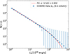 |
Fig. 6. Cumulative XLF of simulated ULX population at 40% of Z⊙ in the 0.2−12 keV band. |
Walton et al. (2011) constructed XLFs for observed ULXs in spiral and elliptical galaxies and found α = 1.85 ± 0.11 and a steeper index of α = 2.5 ± 0.4 for the two galaxy types, respectively. Salvaggio et al. (2023) studied the XLF of ULXs found in the Cartwheel galaxy and found a slope of  . Our simulated power-law indices (beamed and non-beamed) fall within the uncertainties of the indices reported for the observed data by these authors.
Table 4 presents the α, Ls, and β in Eq. (17) for XLF of ULXs at different metallicities, including the effects of beaming. These parameters highlight the significant impact of beaming on the observed properties of ULX populations. The slope α, which characterises the distribution of ULX luminosities, shows a notable difference between the beamed and non-beamed cases. With a constant θf = 45° (Table 1), the slope α is consistently steeper across all metallicities – ranging from 1.77 to 2.15 – indicating a rapid decline in the number of high-luminosity ULXs. In contrast, with beaming (Table 4), the slope remains nearly constant across all metallicities.
XLF fit parameters with beaming included.
The dependence of N(LX) on the beaming angle θf flattens the slope of the XLF and reduces its sensitivity to metallicity. Hence, beaming masks the underlying variations in mass distributions across metallicities that would otherwise steepen the XLF, as higher metallicities tend to produce lower mass compact objects in the case of black holes.
With beaming, Ls values are generally higher. For instance, at 0.5% of Z⊙, Ls = 218 × 1039 erg s−1, which is much higher than Ls = 59.5 × 1039 erg s−1 with θf = 45° and at 0.5% of Z⊙.
The introduction of beaming also impacts the optical–X-ray spectral index, αox. Figure 7 presents αox as a function of Lν,UV (2500 Å luminosity) for our simulated ULX population, including beaming. The slopes (m) of the αox versus Lν,UV relation differ significantly between the beamed (Table 5) and non-beamed ones (Table 2) at high metallicity, highlighting the substantial impact of beaming on the relative X-ray and UV emissions of ULXs.
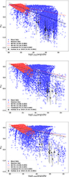 |
Fig. 7. αox index as function of Lν,UV (2500 Å) luminosity for our simulated ULX population (BH or NS primaries) with beaming included in the calculation. The best fit to αox − Lν,UV simulated data in our population (black solid line) and observed ULX data in Sonbas et al. (2019) (black points) are also shown. The top, middle, and bottom panels correspond to metallicities of 0.25 Z⊙, 0.2 Z⊙, and 0.4 Z⊙, respectively. |
Slope of αox versus Lν,UV with beaming included.
Including beaming leads to high-beamed systems resulting in more positive αox values compared to the observational data and, hence, more data points lying above those of Sonbas et al. (2019). In general, introducing beaming reduces the magnitude of the slope, m, particularly at higher metallicities. This suggests that at higher metallicities, beaming results in a larger number of systems with focused emission, leading to a flattening of the αox − Lν,UV relation. As a result, metallicity plays a diminished role in determining the observed correlation, with beaming effects becoming the dominant factor influencing the properties of these ULX systems. Furthermore, we notice that the inclusion of beaming leads to a large scatter in the αox − Lν,UV plane and a linear fit may not be appropriate as can be inferred from the near-flat slope of the fits.
4.3.2. Neutron star ULXs
Pulsations found in some ULX systems have provided compelling evidence that at least a fraction of ULXs are powered by NSs (Bachetti et al. 2014; Fürst et al. 2016). In Fig. 8, we present the XLF of our simulated NS-ULX population at Z = 40% Z⊙. Our simulations reveal that the XLF of NS-ULXs has a slope similar to that of the total ULX population, though with slightly higher Ls and β; values in Fig. 8 are given by 381 ± 29 × 1039 erg s−1 and 1.3 ± 0.1, respectively.
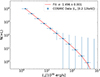 |
Fig. 8. Cumulative XLF of simulated NS-ULX population at 40% of Z⊙ in the 0.2−12 keV band including beaming. |
We find that the average value of θf ≈ 22° for all NS-ULXs at Z = 40% Z⊙, which corresponds to 1/b ≈ 13. Therefore, a beaming factor of at least 10 is required to achieve extreme luminosities (LX > 1040 erg/s) observed in some NS-ULXs. However, the high pulsed fractions observed in some pulsating ULXs (Bachetti et al. 2022) give a strong argument against strong beaming in these systems (Mushtukov et al. 2021). Furthermore, Bachetti et al. (2022) showed that the extreme luminosity of M82 X-2 can be explained by super-Eddington accretion and high mass-transfer rates onto a highly magnetised NS.
The omission of magnetic fields from our model presents a limitation. Including the magnetic field can significantly affect the accretion geometry and emission properties of the NS-ULX systems (e.g. Middleton et al. 2019; Mushtukov et al. 2021; Bachetti et al. 2022). Incorporating these effects is, however, beyond the scope of this work.
4.3.3. Observable ULX population
Beamed emission from a ULX is observable if the observer’s line of sight is within θf. To study what fraction of our ULX population is observable, we assigned a random viewing angle (β) to all ULXs using the distribution P(β) = sin(β). The cumulative distribution function (CDF) of P(β) is then
Here, C(β) ranges from 0 (at β = 0) to 1 (at β = π) and β = 0 in a face-on case, and β = π/2 is an edge-on case. Therefore,

We used Eq. (24) to calculate β, where C is randomly sampled from a uniform distribution in [0, 1]. A ULX is observable if θf > β or θf > π − β.
Table 6 shows the percentage of ULX population observable after viewing angle correction. A relatively small fraction (≲10%) of the NS ULXs are observable as compared to the BH ULXs. Notably, the NS-ULX fraction remains largely independent of metallicity, while the BH ULXs exhibit a much higher fraction, ranging from 43% at 0.5% Z⊙ to 78% at 150% Z⊙. This difference in the observability of the NS ULXs and BH ULXs can be understood from their beaming distributions shown in Fig. A.7.
Observable ULX population.
Although the fraction of observable ULXs remains below 44% across all metallicities, their properties are not substantially different from those of the entire simulated population. Figure 9 displays the luminosity function of the observable ULXs at 40% Z⊙, while Fig. 11 presents their αox − Lν,UV relation. The observable population shows a slightly steeper αox − Lν,UV slope. It is important to note, however, that our analysis of the observable population does not account for any plausible selection effects of the detector.
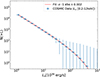 |
Fig. 9. Cumulative XLF of simulated observable ULXs at 40% of Z⊙ in the 0.2−12 keV band including beaming. |
To investigate the effect of selection criteria on the XLF, we computed the selection probability as a function of luminosity. To calculate this probability, we divided the luminosity range into logarithmically spaced bins and computed the total number of systems and the number of observable systems in each bin. The selection probability is then defined as the ratio of the observable to the total number of systems.
Figure 10 shows the selection probability for the population in Fig. 6 and the observable population in Fig. 9. The results reveal that the probability remains approximately flat between 1039 and 2 × 1040 erg s−1, and this is where most of the ULX systems are located.
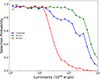 |
Fig. 10. Selection probability, ratio of the observable to the total number of all ULX systems (blue), BH-ULX (green), and NS-ULX (red), as a function of X-ray luminosity at 40% Z⊙. |
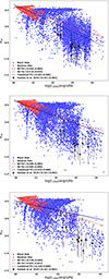 |
Fig. 11. αox versus Lν,UV (2500 Å) for our simulated observable ULX population (BH or NS primaries) with beaming included in the calculation. The best fit to the simulated data (black solid line) and observed ULXs in Sonbas et al. (2019) (black points) are also shown. The top, middle, and bottom panels correspond to metallicities of 0.25 Z⊙, 0.2 Z⊙, and 0.4 Z⊙, respectively. |
The invariance of the XLF slope is primarily driven by the dominance of ULX systems within the flat-probability range in Fig. 10. In this region, the probability of making an observation is high due to low beaming, which results in a wider opening angle. At high luminosities (L > 2 × 1040 erg s−1), the NS-ULX emission becomes increasingly beamed into narrow cones, significantly reducing the likelihood of observation and resulting in a drop in the total probability. In contrast, the BH-ULX selection probability remains constant below luminosities of L ∼ 1041 erg s−1, where beaming is unimportant.
The selection process does not introduce significant luminosity-dependent biases in this range, allowing the intrinsic XLF properties to be preserved in the observed sample. It is also important to remind the reader that the viewing angle is randomly assigned from a sin(β) distribution. Hence, the luminosity does not depend on the angle β.
5. Summary and conclusions
We summarise our results below.
-
In this study, we used the COSMIC population synthesis code to simulate the evolution of binary systems and investigate the relationship between UV and X-ray emission during the ULX phase.
-
We adopted the SCAD model by Vinokurov et al. (2013) to calculate the SEDs of our simulated ULX population from the accretion disc. While X-rays are emitted solely by the accretion disc, the UV emission is a combination of heated wind from the disc and the surface emission from the companion star.
-
Our findings indicate that the number of ULXs decreases with increasing metallicity, which is consistent with observational data. We found that BH-ULXs decrease at a faster rate than NS-ULXs with increasing metallicity and obtained a power-law index of α = 0.16 ± 0.01 for the combined population of BH- and NS-ULXs, which is consistent with values reported in the literature. The decreasing number of ULXs with increasing metallicity has significant implications for our understanding of ULX populations in different galactic environments. In metal-poor galaxies, we expect a higher number of ULXs, which can serve as important probes of early galaxy evolution.
-
Luminosity Function: the XLF slopes of our simulated ULX population vary with metallicity; that is, with lower metallicity populations exhibiting a relative excess of high-luminosity ULXs. Without beaming, the slope ranges from α = 1.77 ± 0.01 at 0.5% solar metallicity to α = 2.15 ± 0.38 at 1.5 times solar metallicity. The inclusion of beaming flattens the XLF slope across all metallicities, reflecting the boosted luminosity due to the beaming effect. Our simulated slopes are consistent with observational data from Walton et al. (2011) and Salvaggio et al. (2023), who reported similar values for ULXs in different types of galaxies.
-
The optical–X-ray spectral index αox showed a significant anti-correlation with UV luminosity across different metallicities. This relation is found using both the disc and the stellar companion contributions to the UV emission. Our results suggest that UV emission in ULXs is predominantly disc-dominated, with the percentage of disc-dominated ULXs increasing as metallicity rises. The slope of the αox − Lν,UV relation for BH-ULXs changes with metallicity; it becomes steeper at higher metallicities, while the slope for NS-ULXs remains relatively constant. With beaming included, the slopes of the αox − Lν,UV relation become significantly flatter and remain relatively constant with metallicity.
-
For a constant θf, our results suggest that the majority of the ULXs with unique optical counterparts selected by Sonbas et al. (2019) are likely powered by black holes when fout = 0.03; however, for high fout > 0.1 more NS-ULX systems are found to be compatible with the observational data. Including beaming in our calculation resulted in high αox values compared to Sonbas et al. (2019) data points.
-
Our results support the hypothesis that stellar-mass BHs and NSs, undergoing supercritical accretion, can account for the observed properties of ULXs without necessitating the presence of IMBHs.
-
While the X-ray emission remains unaffected, higher wind velocity reduces UV emission, causing the αox values to become more positive.
-
Due to their high beaming, NS-ULX systems produce narrow emission cones, which significantly reduce their likelihood of being observed.
We note that COSMIC has a few limitations in simulating the evolution of binary populations. For example, the relationship between remnant mass and initial mass or carbon-oxygen core mass is not always straightforward. Other theoretical models have shown that some massive stars directly implode into black holes without an explosion (Patton & Sukhbold 2020), which COSMIC does not fully account for. Unlike advanced stellar evolution codes such as Modules for Experiments in Stellar Astrophysics (MESA; Paxton et al. 2011), which provides detailed simulations of the physical processes governing the life cycle of stars, COSMIC is a rapid population-synthesis code that relies on simplified models for stellar and binary evolution, introducing systematic biases in the resulting binary populations (Marchant et al. 2021; Gallegos-Garcia et al. 2021). These limitations can be addressed by population synthesis codes such as POSYDON (Fragos et al. 2023), which incorporate a detailed MESA code. However, current versions of these codes are constrained to a limited range of metallicity and are not yet suitable for studies similar to ours, where metallicity is varied over a wide range.
We also note a few limitations of our radiation calculations. The SCAD model has been developed for BH-ULX systems. Its application to NS-ULX systems in our study is limited. One significant issue is that we did not account for the effects of magnetic fields in NS-ULX systems. Magnetic fields can play a critical role in the dynamics of the accretion disc, potentially leading to disc truncation and the occurrence of pulsations, both of which are characteristic features of NS-ULXs (Middleton et al. 2019). Calculations by Mushtukov et al. (2021) suggest that strong magnetic fields (B > 1013 G) in systems such as M82 X-2 facilitate super-Eddington accretion and reduce reliance on beaming to achieve high luminosities. Similarly, Bachetti et al. (2022) argued that moderate beaming combined with accretion funnel effects and magnetic-field interactions better explain the observed properties of pulsating ULXs. Additionally, the irradiation of the donor star by the accretion disc, which can increase UV emission (Motch et al. 2014), was not considered, potentially affecting the accuracy of the αox versus Lν,UV relation. Our future studies will aim to improve on some of those limitations.
Data availability
Appendix A, which includes Figs. A.1 through A.7, is available on Zenodo: https://doi.org/10.5281/zenodo.14715088
Appendix A is available at https://doi.org/10.5281/zenodo.14715088
Acknowledgments
We are grateful to the referee for helpful comments that have improved this paper. We would like to thank Kalvir Dhuga, Eda Sonbas and Andrzej Zdziarski for helpful discussions. L.N. is grateful to Katelyn Breivik for advice on the COSMIC code. L.N. and S.R. were partially supported by a BRICS STI grant and by a NITheCS grant from the National Research Foundation, South Africa. J.D.F. was supported by NASA through contract S-15633Y and the Office of Naval Research.
References
- Bachetti, M., Harrison, F., Walton, D. J., et al. 2014, Nature, 514, 202 [NASA ADS] [CrossRef] [Google Scholar]
- Bachetti, M., Heida, M., Maccarone, T., et al. 2022, ApJ, 937, 125 [NASA ADS] [CrossRef] [Google Scholar]
- Begelman, M. C. 2001, ApJ, 551, 897 [NASA ADS] [CrossRef] [Google Scholar]
- Belczynski, K., Taam, R. E., Kalogera, V., Rasio, F. A., & Bulik, T. 2007, ApJ, 662, 504 [Google Scholar]
- Belczynski, K., Kalogera, V., Rasio, F. A., et al. 2008, ApJS, 174, 223 [Google Scholar]
- Breivik, K., Coughlin, S., Zevin, M., et al. 2020, ApJ, 898, 71 [Google Scholar]
- Brown, G. E., Lee, C. H., Wijers, R. A. M. J., et al. 2000, New Astron., 5, 191 [NASA ADS] [CrossRef] [Google Scholar]
- Colbert, E. J. M., & Mushotzky, R. F. 1999, ApJ, 519, 89 [NASA ADS] [CrossRef] [Google Scholar]
- Fabbiano, G. 1989, ARA&A, 27, 87 [NASA ADS] [CrossRef] [Google Scholar]
- Finke, J. D., & Böttcher, M. 2007, ApJ, 667, 395 [NASA ADS] [CrossRef] [Google Scholar]
- Finke, J. D., & Razzaque, S. 2017, MNRAS, 472, 3683 [NASA ADS] [CrossRef] [Google Scholar]
- Fragos, T., Andrews, J. J., Bavera, S. S., et al. 2023, ApJS, 264, 45 [NASA ADS] [CrossRef] [Google Scholar]
- Fryer, C. L., Belczynski, K., Wiktorowicz, G., et al. 2012, ApJ, 749, 91 [Google Scholar]
- Fürst, F., Walton, D. J., Harrison, F. A., et al. 2016, ApJ, 831, L14 [Google Scholar]
- Gallegos-Garcia, M., Berry, C. P. L., Marchant, P., & Kalogera, V. 2021, ApJ, 922, 110 [NASA ADS] [CrossRef] [Google Scholar]
- Georganopoulos, M., Aharonian, F. A., & Kirk, J. G. 2002, A&A, 388, L25 [NASA ADS] [CrossRef] [EDP Sciences] [Google Scholar]
- Gierliński, M., Done, C., & Page, K. 2008, MNRAS, 388, 753 [Google Scholar]
- Gierliński, M., Done, C., & Page, K. 2009, MNRAS, 392, 1106 [CrossRef] [Google Scholar]
- Gladstone, J. C., Copperwheat, C., Heinke, C. O., et al. 2013, ApJS, 206, 14 [NASA ADS] [CrossRef] [Google Scholar]
- Heger, A., Fryer, C. L., Woosley, S. E., Langer, N., & Hartmann, D. H. 2003, ApJ, 591, 288 [CrossRef] [Google Scholar]
- Heida, M., Torres, M. A. P., Jonker, P. G., et al. 2015, MNRAS, 453, 3510 [Google Scholar]
- Heida, M., Lau, R. M., Davies, B., et al. 2019, ApJ, 883, L34 [NASA ADS] [CrossRef] [Google Scholar]
- Inoue, Y., Tanaka, Y. T., & Isobe, N. 2016, MNRAS, 461, 4329 [NASA ADS] [CrossRef] [Google Scholar]
- Kaaret, P., Feng, H., & Roberts, T. P. 2017, ARA&A, 55, 303 [Google Scholar]
- King, A. R. 2009, MNRAS, 393, L41 [NASA ADS] [Google Scholar]
- King, A. R., Davies, M. B., Ward, M. J., Fabbiano, G., & Elvis, M. 2001, ApJ, 552, L109 [NASA ADS] [CrossRef] [Google Scholar]
- King, A., Lasota, J.-P., & Middleton, M. 2023, New Astron. Rev., 96, 101672 [CrossRef] [Google Scholar]
- Kosec, P., Pinto, C., Walton, D. J., et al. 2018, MNRAS, 479, 3978 [NASA ADS] [Google Scholar]
- Kroupa, P., Tout, C. A., & Gilmore, G. 1993, MNRAS, 262, 545 [NASA ADS] [CrossRef] [Google Scholar]
- Lasota, J. P., Alexander, T., Dubus, G., et al. 2011, ApJ, 735, 89 [NASA ADS] [CrossRef] [Google Scholar]
- Lasota, J.-P., Vieira, R., Sadowski, A., Narayan, R., & Abramowicz, M. 2016, A&A, 587, A13 [NASA ADS] [CrossRef] [EDP Sciences] [Google Scholar]
- Lehmer, B. D., Eufrasio, R. T., Basu-Zych, A., et al. 2021, ApJ, 907, 17 [NASA ADS] [CrossRef] [Google Scholar]
- Liu, J.-F., Bregman, J. N., & Seitzer, P. 2004, ApJ, 602, 249 [NASA ADS] [CrossRef] [Google Scholar]
- Mapelli, M., Ripamonti, E., Zampieri, L., & Colpi, M. 2011, Astron. Nachr., 332, 414 [NASA ADS] [CrossRef] [Google Scholar]
- Marchant, P., Pappas, K. M. W., Gallegos-Garcia, M., et al. 2021, A&A, 650, A107 [NASA ADS] [CrossRef] [EDP Sciences] [Google Scholar]
- McKinney, J. C., Tchekhovskoy, A., Sadowski, A., & Narayan, R. 2014, MNRAS, 441, 3177 [NASA ADS] [CrossRef] [Google Scholar]
- Mezcua, M., Roberts, T., Sutton, A., & Lobanov, A. 2013, MNRAS, 436, 3128 [NASA ADS] [CrossRef] [Google Scholar]
- Middleton, M. J., Miller-Jones, J. C., Markoff, S., et al. 2013, Nature, 493, 187 [NASA ADS] [CrossRef] [Google Scholar]
- Middleton, M. J., Heil, L., Pintore, F., Walton, D. J., & Roberts, T. P. 2015, MNRAS, 447, 3243 [Google Scholar]
- Middleton, M., Brightman, M., Pintore, F., et al. 2019, MNRAS, 486, 2 [NASA ADS] [Google Scholar]
- Mitsuda, K., Inoue, H., Koyama, K., et al. 1984, PASJ, 36, 741 [NASA ADS] [Google Scholar]
- Mondal, S., Belczyński, K., Wiktorowicz, G., Lasota, J.-P., & King, A. R. 2020, MNRAS, 491, 2747 [Google Scholar]
- Motch, C., Pakull, M., Soria, R., Grisé, F., & Pietrzyński, G. 2014, Nature, 514, 198 [NASA ADS] [CrossRef] [Google Scholar]
- Murdin, P., & Webster, B. L. 1971, Nature, 233, 110 [NASA ADS] [CrossRef] [Google Scholar]
- Mushtukov, A. A., Portegies Zwart, S., Tsygankov, S. S., Nagirner, D. I., & Poutanen, J. 2021, MNRAS, 501, 2424 [NASA ADS] [CrossRef] [Google Scholar]
- Patton, R. A., & Sukhbold, T. 2020, MNRAS, 499, 2803 [NASA ADS] [CrossRef] [Google Scholar]
- Paxton, B., Bildsten, L., Dotter, A., et al. 2011, ApJS, 192, 3 [Google Scholar]
- Pinto, C., & Walton, D. J. 2023, ArXiv e-prints [arXiv:2302.00006] [Google Scholar]
- Pinto, C., Walton, D., Kara, E., et al. 2020, MNRAS, 492, 4646 [NASA ADS] [CrossRef] [Google Scholar]
- Poutanen, J., Lipunova, G., Fabrika, S., Butkevich, A. G., & Abolmasov, P. 2007, MNRAS, 377, 1187 [NASA ADS] [CrossRef] [Google Scholar]
- Roberts, T., Levan, A., & Goad, M. 2008, MNRAS, 387, 73 [CrossRef] [Google Scholar]
- Sądowski, A., & Narayan, R. 2015, MNRAS, 453, 3213 [Google Scholar]
- Salvaggio, C., Wolter, A., Belfiore, A., & Colpi, M. 2023, MNRAS, 522, 1377 [NASA ADS] [CrossRef] [Google Scholar]
- Sana, H., de Koter, A., De Mink, S., et al. 2013, A&A, 550, A107 [NASA ADS] [CrossRef] [EDP Sciences] [Google Scholar]
- Shakura, N. I., & Sunyaev, R. A. 1973, A&A, 24, 337 [NASA ADS] [Google Scholar]
- Sonbas, E., Dhuga, K. S., & Göğüş, E. 2019, ApJ, 873, L12 [NASA ADS] [CrossRef] [Google Scholar]
- Tananbaum, H., Avni, Y., Branduardi, G., et al. 1979, ApJ, 234, L9 [Google Scholar]
- Tao, L., Feng, H., Kaaret, P., Grisé, F., & Jin, J. 2012, ApJ, 758, 85 [NASA ADS] [CrossRef] [Google Scholar]
- Vagnozzi, S., Freese, K., & Zurbuchen, T. H. 2017, ApJ, 839, 55 [NASA ADS] [CrossRef] [Google Scholar]
- Van Den Eijnden, J., Degenaar, N., Schulz, N., et al. 2019, MNRAS, 487, 4355 [NASA ADS] [CrossRef] [Google Scholar]
- Vasilopoulos, G., Ray, P., Gendreau, K., et al. 2020, MNRAS, 494, 5350 [NASA ADS] [CrossRef] [Google Scholar]
- Vinokurov, A., Fabrika, S., & Atapin, K. 2013, Astrophys. Bull., 68, 139 [NASA ADS] [CrossRef] [Google Scholar]
- Walton, D., Roberts, T., Mateos, S., & Heard, V. 2011, MNRAS, 416, 1844 [NASA ADS] [CrossRef] [Google Scholar]
- Walton, D., Mackenzie, A., Gully, H., et al. 2022, MNRAS, 509, 1587 [Google Scholar]
- Wiktorowicz, G., Sobolewska, M., Lasota, J.-P., & Belczynski, K. 2017, ApJ, 846, 17 [NASA ADS] [CrossRef] [Google Scholar]
All Tables
All Figures
|
Fig. 1. Number of ULXs formed in our simulation (NULX) as a function of metallicity. The y-axis indicates the number of ULXs derived from the simulations, with emphasis placed on the trend’s shape rather than the absolute values. The solid lines represent fits to the simulated data, with the corresponding slopes mentioned in the legend. |
| In the text | |
|
Fig. 2. Cumulative XLF of the simulated ULX population at 40% Z⊙ in the 0.2−12 keV band. |
| In the text | |
|
Fig. 3. Spectra of three BH-ULX and three NS-ULX systems from our simulation, showing the mass of the compact object (M) and the ratio ṁ = Ṁ/ṀEdd. Flux is calculated for all systems located at 3 Mpc, and for all curves fout = 0.03 and θf = 45°. |
| In the text | |
|
Fig. 4. αox index as function of Lν,UV (2500 Å) luminosity for our simulated ULX population (BH or NS primaries). The best fit to αox − Lν,UV simulated data in our population (black solid line) and observed ULXs data in Sonbas et al. (2019) (black points) are also shown. The top, middle, and bottom panels correspond to metallicities of 0.025 Z⊙, 0.20 Z⊙, and 0.40 Z⊙, respectively. We also show the αox − Lν,UV fits for the BH-ULX and NS-ULX systems separately. |
| In the text | |
|
Fig. 5. αox for donor-star-dominated UV emission for ULX systems as a function of UV (2500 Å) luminosity for our simulated ULX population (BH or NS primaries). The best fit to αox − Lν,UV simulated data in our population (black solid) at 0.2 Z⊙ and that for observed ULXs in Sonbas et al. (2019) (black points) are also shown. |
| In the text | |
|
Fig. 6. Cumulative XLF of simulated ULX population at 40% of Z⊙ in the 0.2−12 keV band. |
| In the text | |
|
Fig. 7. αox index as function of Lν,UV (2500 Å) luminosity for our simulated ULX population (BH or NS primaries) with beaming included in the calculation. The best fit to αox − Lν,UV simulated data in our population (black solid line) and observed ULX data in Sonbas et al. (2019) (black points) are also shown. The top, middle, and bottom panels correspond to metallicities of 0.25 Z⊙, 0.2 Z⊙, and 0.4 Z⊙, respectively. |
| In the text | |
|
Fig. 8. Cumulative XLF of simulated NS-ULX population at 40% of Z⊙ in the 0.2−12 keV band including beaming. |
| In the text | |
|
Fig. 9. Cumulative XLF of simulated observable ULXs at 40% of Z⊙ in the 0.2−12 keV band including beaming. |
| In the text | |
|
Fig. 10. Selection probability, ratio of the observable to the total number of all ULX systems (blue), BH-ULX (green), and NS-ULX (red), as a function of X-ray luminosity at 40% Z⊙. |
| In the text | |
|
Fig. 11. αox versus Lν,UV (2500 Å) for our simulated observable ULX population (BH or NS primaries) with beaming included in the calculation. The best fit to the simulated data (black solid line) and observed ULXs in Sonbas et al. (2019) (black points) are also shown. The top, middle, and bottom panels correspond to metallicities of 0.25 Z⊙, 0.2 Z⊙, and 0.4 Z⊙, respectively. |
| In the text | |
Current usage metrics show cumulative count of Article Views (full-text article views including HTML views, PDF and ePub downloads, according to the available data) and Abstracts Views on Vision4Press platform.
Data correspond to usage on the plateform after 2015. The current usage metrics is available 48-96 hours after online publication and is updated daily on week days.
Initial download of the metrics may take a while.