| Issue |
A&A
Volume 694, February 2025
|
|
|---|---|---|
| Article Number | L4 | |
| Number of page(s) | 7 | |
| Section | Letters to the Editor | |
| DOI | https://doi.org/10.1051/0004-6361/202453428 | |
| Published online | 04 February 2025 | |
Letter to the Editor
Testing a proposed planarity tool for studying satellite systems
The alleged consistency of Milky Way satellite galaxy planes with ΛCDM
1
Leibniz-Institute for Astrophysics Potsdam (AIP), An der Sternwarte 16, 14482 Potsdam, Germany
2
Institut für Physik und Astronomie, Universität Potsdam, Karl-Liebknecht-Straße 24/25, D-14476 Potsdam, Germany
3
Institute of Physics, Laboratory of Astrophysics, Ecole Polytechnique Fédérale de Lausanne (EPFL), 1290 Sauverny, Switzerland
⋆ Corresponding author; mpawlowski@aip.de
Received:
13
December
2024
Accepted:
30
December
2024
Context. The existence of planes of satellite galaxies has been identified as a long-standing challenge to ΛCDM cosmology because satellite systems in cosmological simulations that are as extremely flattened and as strongly kinematically correlated as the observed structures are rare.
Aims. We investigate a recently proposed new metric for measuring the overall degree of planarity of a satellite system that was used to claim consistency between the Milky Way satellite plane and ΛCDM.
Methods. We studied the behavior of the planarity metric under several features of anisotropy that are present in ΛCDM satellite systems but are not related to satellite planes. Specifically, we considered the impact of oblate or prolate distributions, the number of satellites, the clustering of satellites, and radial and asymmetric distributions (lopsidedness). We also investigated whether the metric is independent of the orientation of the studied satellite system.
Results. We find that all of these features of anisotropy lead to the metric to infer an increased degree of planarity, even though none of them has any direct relation to satellite planes. The metric is also highly sensitive to the orientation of the studied system (or chosen coordinate system): There is almost no correlation between the reported degrees of planarity of the metric for identical random systems rotated by 90°.
Conclusions. Our results demonstrate that the new proposed metric is not suited for measuring the overall planarity in satellite systems. Consequently, no consistency of the observed Milky Way satellite plane with ΛCDM can be inferred using this metric.
Key words: methods: data analysis / Galaxy: formation / galaxies: dwarf / galaxies: evolution / galaxies: structure
© The Authors 2025
 Open Access article, published by EDP Sciences, under the terms of the Creative Commons Attribution License (https://creativecommons.org/licenses/by/4.0), which permits unrestricted use, distribution, and reproduction in any medium, provided the original work is properly cited.
This article is published in open access under the Subscribe to Open model. Subscribe to A&A to support open access publication.
1. Introduction
Observational evidence for the presence of planes of satellite galaxies that likely co-orbit has been demonstrated for numerous systems (see Pawlowski 2018 for a review). Well-studied cases include the Milky Way (Kroupa et al. 2005; Pawlowski et al. 2012; Taibi et al. 2024), M31 (Ibata et al. 2013; Sohn et al. 2020), Centaurus A (Tully et al. 2015; Müller et al. 2018; Kanehisa et al. 2023), and NGC4490 (Karachentsev & Kroupa 2024). For these observed systems, analogs with similar degrees of spatial flattening and kinematic coherence are rare in ΛCDM simulations (Ibata et al. 2014; Pawlowski & McGaugh 2014; Forero-Romero & Arias 2018; Pawlowski et al. 2019; Müller et al. 2021; Pawlowski & Tony Sohn 2021; Samuel et al. 2021; Pawlowski et al. 2024; Seo et al. 2024).
Other observed host galaxies also show some signs of possible planarity1 or kinematic coherence in their associated satellites, but the degree of their difference with cosmological expectations is less well established (e.g., Chiboucas et al. 2013; Paudel et al. 2021; Martínez-Delgado et al. 2021; Müller et al. 2024; Mutlu-Pakdil et al. 2024; Martinez-Delgado et al. 2024).
Spatial flattening is commonly measured as the major-to-minor axis ratio in 2D, or the absolute root-mean-square plane height in 3D. The kinematic coherence is either measured as the dispersion of orbital poles when the 3D velocities are known from proper motions, or as 2D line-of-sight velocity trends for more distant systems. In the presence of well-established methods that are used widely by many different teams, the introduction of new metrics for measuring satellite planes (Shao et al. 2019; Förster et al. 2022; Seo et al. 2024) can hinder comparability. When a novel tool is also only applied to a new simulation, it prevents us from assessing whether an apparent consistency between the observation and simulation arises because the latter is more successful in reproducing the observed system than previous simulations, or if it is due to shortcomings of the new metric (which often affect these proposed new analysis tools; see, e.g., Pawlowski et al. 2014, 2015, 2017a; Pawlowski & Kroupa 2020).
We therefore need to ensure that the tools we apply are suitable and have been demonstrated to reliably measure what we wish them to measure. A good tool needs to have both a high sensitivity and a high specificity. The former implies that the tool can accurately diagnose a property present in the data (e.g., the presence of planes in the distribution of satellite galaxies), while the latter requires that the tool does not return false-positive diagnoses in the absence of the condition being tested for (e.g., reporting high degrees of planarity for systems without intrinsic planes).
Uzeirbegovic et al. (2024) have recently proposed yet another new tool that is aimed at measuring the overall “planarity” present in a system of satellite galaxies. The metric intends to measure with a single value the overall degree of planarity in a distribution. Their new tool does return high degrees of “planarity” not only for the distribution of Milky Way satellite galaxies, but also for a range of satellite systems extracted from the NewHorizon cosmological simulation (Dubois et al. 2021). Uzeirbegovic et al. (2024) interpreted this as demonstrating consistency between ΛCDM expectations and the observed system and its satellite plane.
By generating one mock satellite system in which satellite subsamples are confined to three planes, Uzeirbegovic et al. (2024) demonstrated the tool’s sensitivity to the presence of planar distributions. However, reverse tests investigating the specificity were not presented. It is thus unclear whether the proposed tool is a suitable metric for reliably measuring “planarity”, or if it might instead be affected by other influences, such as different types of deviations of the satellite systems from isotropy.
In the following, we investigate the metric and its response to several types of phase-space correlations present in satellite galaxy systems, both observed in the Universe and extracted from ΛCDM simulations. We show that the proposed metric lacks specificity, since it is sensitive to other anisotropies (oblate or prolate distributions, clustering, and lopsidedness) that are independent of the presence of planar arrangements. This result is contrary to its intended purpose. We also demonstrate that the degree of “planarity” it returns is affected by the orientation of its coordinate system relative to the studied satellite distribution. We refrain from commenting on the application of the metric on velocity vectors because the following investigations of positions alone already disqualify it from further use. However, we note that the procedure employed by Uzeirbegovic et al. (2024) to sample from the measurement uncertainties of observed satellite galaxy positions and velocities, namely sampling them in 6D Cartesian coordinates independently, ignores the strong correlations between them and results in nonphysical satellite phase-space positions (see Appendix A).
We note that Uzeirbegovic et al. (2024) required each host to contain more than 30 satellites with stellar masses > 105 M⊙, while considering hosts with a stellar mass > 1010 M⊙. Given that for the Milky Way we know of only 15 satellites that exceed this stellar mass (Pace 2024), it appears plausible that many simulated hosts might be more massive than the Milky Way. Because no information on the host mass distributions or the number of satellites per host is provided in Uzeirbegovic et al. (2024), we cannot make definitive statements on this issue, however.
2. Investigating the “planarity” metric
The metric proposed by Uzeirbegovic et al. (2024) constructs the cross-products of all possible combinations of satellite galaxy position vectors2. It thus collects all plane normal vectors defined by any combination of two satellites and the center of the coordinate system, which is chosen as the host galaxy position.
These normal vectors are expressed in spherical coordinates and were binned in m bins in azimuth and inclination. The resulting 2D histogram of normal-vector counts per bin was summarized by calculating the Gini coefficient of all bin values. The same was done for 1000 random mock systems, with positions drawn from an isotropic distribution. For a given satellite system under study, its degree of “planarity” is reported as the quantile value of its Gini coefficient relative to the distribution of Gini coefficients of these random systems. Uzeirbegovic et al. (2024) reported that the Milky Way system and most of the simulated satellite systems return very high quantiles, which they interpreted as consistency between the observed satellite plane and ΛCDM.
The reliance on a spherical coordinate system that is binned in angles implies a special direction in the analysis: the pole of this coordinate system. The orientation of this direction must not affect the output of the metric. After all, the presence of planes in a system needs to be measured independently of the orientation under which the system is studied.
Furthermore, different types of phase-space correlations beyond planes are present in observed satellite systems and in those obtained from cosmological simulations (for a review, see Pawlowski 2021). A metric for measuring planarity therefore needs to demonstrate that it does, in fact, measure planarity, and not, for example, just a general deviation from isotropy. This requires testing whether the metric is affected by other phase-space correlations that are independent of the issue of satellite planes.
Since no such tests were presented by Uzeirbegovic et al. (2024), we set out to do this with a number of toy-model systems. For this purpose, we used the code made publicly available by the authors3. We note that while Uzeirbegovic et al. (2024) described that the spherical coordinates were scaled to ensure that all bins had an equal area, no such scaling is apparent in the provided code. Since we thus cannot be sure which procedure was applied, we used the provided code by default, but we repeat our analysis in Appendix B after implementing such a scaling. Our main conclusions apply to either case.
Unless stated otherwise, we followed their fiducial choices: m = 25 bins per angular dimension, and 1000 isotropic realizations relative to which the quantile of a given system is obtained. We base our comparisons on mock systems with Nsat = 40 satellites, comparable to the number of Milky Way satellites considered in the original study and to their requirement that simulated systems contain Nsat > 30 satellites.
2.1. Effect of orientation or the coordinate system
An essential quality of any suitable metric for measuring the planarity of a satellite system is that it needs to be independent of the overall orientation of the system under study, or of the chosen coordinate system. The metric relies on a 2D histogram of the spherical coordinates of pairwise cross-products of vectors. The statistics of the bin counts, that is, how much they deviate from a distribution expected for random systems, is used to quantify the degree of “planarity”. However, a histogram in two spherical coordinates implies a tighter sampling in azimuth for regions closer to the poles, and it suggests that the orientation of the system might affect the resulting “planarity” measure.
We have tested this concern by investigating 1000 random satellite systems, generated in the same way as by Uzeirbegovic et al. (2024), by drawing from a homogeneously filled unit sphere. This resulted in an isotropic distribution of positions around the origin. For each system, we measured the quantile. As expected, random systems resulted in an overall flat quantile distribution. We then rotated the distributions by 90° around the y-axis, such that the former x-axis lay along the new z-axis direction, and vice versa. This preserved the mutual distributions of the satellites, and only their orientation relative to the z-axis defining the orientation of the histogram was different. We repeated the analysis and again determined the quantiles.
Our results are shown in Fig. 1. The quantiles measured in the two orientations vary strongly, with almost no apparent correlation. This was confirmed by tests for the linear and rank correlation: the Pearson correlation coefficient is r = 0.352, and the Spearman correlation coefficient is ρ = 0.351. A robust metric independent of orientation results in identical quantiles for these rotated systems. The “planarity” metric does not. This already shows that the metric is not suitable for studying the flattening of a satellite system. We have uncovered more issues, however.
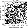 |
Fig. 1. Quantiles for 1000 random isotropic distributions in two orientations rotated by 90°. No strong correlation is apparent, indicating that the output of the proposed ”planarity” metric is sensitive to the orientation of the satellite system under study. |
2.2. Effect of the halo shape
It is well established that dark matter halos in ΛCDM, as well as their associated subhalo and thus satellite galaxy systems, are intrinsically triaxial (Bailin & Steinmetz 2005; Allgood et al. 2006; Wang et al. 2008; Vega-Ferrero et al. 2017). This overall shape does not imply that they contain planes of satellite galaxies, however. Even though an overall oblate system might be considered to be somewhat plane-like and thus can plausibly be expected to yield a stronger degree of inferred planarity, this is not the result of substantial subsample planes as supposedly tested for by the metric. It is thus necessary to test whether the metric is sensitive to the overall shape of the studied systems.
We generated isotropic systems following the fiducial method, but rescaled their x-axis coordinates by multiplying them with a factor q. This produced flattened, oblate distributions for q < 1.0 and stretched, prolate distributions for q > 1.0. We applied the “planarity” metric again in two orientations, with its pole along the z- and the x-axis, respectively. The resulting quantile distributions for 1000 systems generated for each considered q = [0.5, 0.67, 1.0, 1.5, 2.0] are illustrated in the middle column of Fig. 2 for our fiducial Nsat = 40. Here, q = 1.0 corresponds to the fiducial, spherical case of Uzeirbegovic et al. (2024).
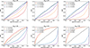 |
Fig. 2. Distribution of quantiles for systems with different degrees of flattening (q < 1.0, oblate) or elongation (q > 1.0, prolate) along the x-axis. From left to right, the number of satellites per system is 20, 40, and 50, respectively. The upper panels orient the metric pole along the z-axis, and the lower panels orient it along the x-axis. |
Our tests showed that prolate distributions result in some deviation in the quantile distribution from isotropy when the direction of stretching and the orientation of the metric pole are perpendicular. Strongly prolate distributions (q = 2) are biased to higher quantile values. Oblate distributions, in contrast, display a more extreme effect and result in a strongly increased number of high-quantile systems. This shows that the proposed ‘planarity’ metric is highly sensitive to the overall shape of the distribution, even in the absence of underlying embedded satellite planes.
Depending on the orientation, however, the metric also displays counterintuitive behavior: When the metric pole aligns with the x-axis (lower panel in Fig. 2), that is, along the direction in which the system is flattened or stretched, then the metric infers a decreased degree of planarity for oblate systems. Their quantile distribution becomes heavily skewed to lower values. The metric appears to infer nonplanarity when the flattening happens to be oriented perpendicular to the poles of the chosen coordinate system. Prolate distributions whose major axis aligns with the pole, in contrast, return very high inferred degrees of planarity because of the strong bias toward large quantiles. Thus, the overall shape of the satellite distribution has a major effect on the quantile returned by the “planarity” metric, which can result in high quantiles even for systems without intrinsic satellite planes. This feature of the metric overestimates the frequency of “planar” systems in cosmological simulations.
2.3. Effect of the number of satellites
Uzeirbegovic et al. (2024) did not require that the number of satellites in the Milky Way sample was matched by its simulated analogs, but only that these analogs had > 30 satellites. While the metric determines the quantile of a given system relative to a sample of isotropic mock systems of the same number, the “planarity” of a system remains sensitive to the number of satellites considered. Any metric that refers to the likelihood that a given configuration appears among its isotropic counterparts needs to account for the fact that given some degree of underlying anisotropy from which the system of interest is drawn, a larger population of satellites will result in a reduced impact of sampling variance and thus a lower likelihood to occur in isotropy.
We tested this by varying the number of satellites drawn from otherwise identical flattened and stretched distributions (as in Sect. 2.2). The results are also shown in Fig. 2 for Nsat = [20, 40, 50]. We identify a strong dependence on the number of satellites, with the same degree of underlying ob- or prolateness resulting in stronger effects on the quantile distribution for systems of larger Nsat. This hinders comparability across different sample sizes, such as between the observed Milky Way satellites and simulated systems.
2.4. Effect of the satellite clustering
Galaxies in ΛCDM cluster hierarchically (White & Rees 1978; White & Frenk 1991). We therefore expect that at least some satellite galaxies have another dwarf companion nearby, be it a current or former satellite (Wheeler et al. 2015; Erkal & Belokurov 2020; Patel et al. 2020; Pawlowski et al. 2022; Müller et al. 2023; Vasiliev 2024), a pair of dwarfs (Evslin 2014; Fattahi et al. 2013; Crnojević et al. 2014; Besla et al. 2018; Chamberlain et al. 2024; Pawlowski et al. 2024), or as part of an infalling group (Wang et al. 2013; Wetzel et al. 2015; Júlio et al. 2024).
This clustering is independent of the presence of satellite planes. It is thus important to test whether satellite clustering affects the inferred planarity. We built a toy model to test this by generating an isotropic system as in the fiducial case, but now each generated satellite had a chance fpair to have a second satellite nearby. For each generated satellite, we drew a random number from a uniform distribution between zero and one. When this was smaller than the probability fpair, then it was a primary of a pair, and we added a secondary satellite nearby. We chose the position of the secondary as an offset from the position of the primary from a flat distribution in all three Cartesian directions, restricted to a maximum range of 10% of the total extent of the system (0.1 for the adopted unit sphere). We stopped the process when, counting primaries and secondaries alike, the total number of requested satellites was reached.
We generated 1000 such systems per fpair = [0.0, 0.1, 0.25, 0.5, 0.75], applied the “planarity” metric, and recorded the resulting quantiles. Figure 3 visualizes the results. Even a mild degree of clustering (one in ten primary satellites was assigned a secondary) leads to a substantial increase in the number of high-quantile cases. Clustering in a galaxy system, a natural occurrence in the hierarchical formation scenario of the ΛCDM model, thus also introduces a strong bias to infer higher degrees of “planarity” with the proposed metric, even in the absence of an underlying satellite plane.
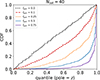 |
Fig. 3. Distribution of quantiles for isotropic distributions with different fractions of paired satellites. Even a mild degree of clustering results in a substantial increase in the high-quantile results. |
2.5. Effect of an asymmetry or a lopsidedness
Observed and simulated systems both show radial distributions with higher satellite densities in the inner than the outer regions (Macciò et al. 2010; Kelley et al. 2019; Samuel et al. 2020). In addition, satellite systems show asymmetries, most prominently, an overall lopsidedness with more satellites on one side of their host than the other (Conn et al. 2013; Libeskind et al. 2016; Brainerd & Samuels 2020; Savino et al. 2022; Heesters et al. 2024). Similar features are present in satellite systems in cosmological simulations (Pawlowski et al. 2017b; Wang et al. 2021; Samuels & Brainerd 2023; Liu et al. 2024). This lopsidedness does not constitute a plane-like satellite distribution, and thus, a metric of planarity should not be sensitive to overall asymmetries or shifts in the satellite distributions.
To test this, we set up model satellite distributions offset from the host and with different radial distributions, as shown in the left panel of Fig. C.1. The fiducial radial distribution of Uzeirbegovic et al. (2024) (dotted black line) assumed a uniform spatial density and resulted in considerably more strongly spread-out satellite distributions than the observed Milky Way system (green line; data from Li et al. 2021 normalized to the most distant considered satellite Leo I).
We generated different distributions by drawing the radial distance of each model satellite from a flat distribution in r′=[0, 1], and we then assigned it a radius r = r′a, with an exponent of a between a = 0.5 (the fiducial radial distribution of Uzeirbegovic et al. 2024), to a = 4 (a highly concentrated distribution). These systems were set up isotropically and were shifted by 10% of their maximum extent along the x-axis (0.1 for the adopted unit sphere). To make them align better with the observed Milky Way satellite system, we rejected satellites within the inner 5% of radius, which would be close to or within the Galactic disk.
The middle and right panels of Fig. C.1 show the resulting quantile distributions. When the metric pole points along the z-axis (perpendicular to the offset), no impact on the quantiles is apparent. However, when the pole aligns with the direction of the offset (the x-axis), then the quantiles are biased to higher values. This effect is stronger for more highly concentrated distributions. Thus, a small asymmetric offset in the satellites and a realistic radially concentrated satellite distribution (natural occurrences in ΛCDM independent of satellite planes) also bias to high inferred quantiles and can thus lead to an incorrect inference of a higher degree of planarity when employing this metric.
3. Conclusions
We have investigated the behavior and properties of the new “planarity” metric proposed by Uzeirbegovic et al. (2024), which they used to claim consistency between the Milky Way plane of satellite galaxies and ΛCDM simulations. We found that the results of the metric are sensitive to the chosen orientation of its spherical coordinate system: The resulting quantile values of mock systems rotated by 90° show almost no correlation. This property alone makes it an inadequate tool for measuring, inferring, or comparing satellite galaxy systems.
Furthermore, we tested the metric response to other types of phase-space correlation present in satellite galaxy systems. We found that the overall deviation of the shape from sphericity, satellite clustering, and lopsided satellite distributions can all result in the proposed “planarity” metric returning high quantile values for mock systems. These features of the metric developed by Uzeirbegovic et al. (2024) will overestimate the inferred occurrence of planes in cosmological simulations. Since all of these effects are present in ΛCDM satellite systems but are independent of the presence of satellite planes, the metric cannot be used to infer the consistency of the Milky Way satellite plane with ΛCDM.
Taken together, we find the proposed “planarity” metric to be unreliable because it is sensitive to the satellite system orientation, and it is biased to return inflated degrees of apparent “planarity” in the presence of other types of phase-space correlations. This results in a lack of specificity. It is thus overall inadequate for studying the problem of planes of satellite galaxies.
In the following, we use the term “planarity” with quotes when it refers to the measure of the specific metric proposed in Uzeirbegovic et al. (2024), while the term without quotes is used when we refer to the general concept of planar arrangements.
In this regard, it is similar to the three- and four-galaxies normal methods of Conn et al. (2013) and Pawlowski et al. (2013), who used these as a discovery tool for identifying possible subsample satellite planes.
Link provided in their paper (last accessed by us on December 12, 2024): https://emiruz.com/vpos, which forwards to https://github.com/emiruz/planarity/
Acknowledgments
Marcel S. Pawlowski acknowledges funding via a Leibniz-Junior Research Group (project number J94/2020). O.M. is grateful to the Swiss National Science Foundation for financial support under the grant number PZ00P2_202104.
References
- Allgood, B., Flores, R. A., Primack, J. R., et al. 2006, MNRAS, 367, 1781 [NASA ADS] [CrossRef] [Google Scholar]
- Bailin, J., & Steinmetz, M. 2005, ApJ, 627, 647 [Google Scholar]
- Battaglia, G., Taibi, S., Thomas, G. F., & Fritz, T. K. 2022, A&A, 657, A54 [NASA ADS] [CrossRef] [EDP Sciences] [Google Scholar]
- Besla, G., Patton, D. R., Stierwalt, S., et al. 2018, MNRAS, 480, 3376 [NASA ADS] [CrossRef] [Google Scholar]
- Brainerd, T. G., & Samuels, A. 2020, ApJ, 898, L15 [NASA ADS] [CrossRef] [Google Scholar]
- Chamberlain, K., Besla, G., Patel, E., et al. 2024, ApJ, 962, 162 [NASA ADS] [CrossRef] [Google Scholar]
- Chiboucas, K., Jacobs, B. A., Tully, R. B., & Karachentsev, I. D. 2013, AJ, 146, 126 [Google Scholar]
- Conn, A. R., Lewis, G. F., Ibata, R. A., et al. 2013, ApJ, 766, 120 [NASA ADS] [CrossRef] [Google Scholar]
- Crnojević, D., Sand, D. J., Caldwell, N., et al. 2014, ApJ, 795, L35 [CrossRef] [Google Scholar]
- Dubois, Y., Beckmann, R., Bournaud, F., et al. 2021, A&A, 651, A109 [NASA ADS] [CrossRef] [EDP Sciences] [Google Scholar]
- Erkal, D., & Belokurov, V. A. 2020, MNRAS, 495, 2554 [NASA ADS] [CrossRef] [Google Scholar]
- Evslin, J. 2014, MNRAS, 440, 1225 [NASA ADS] [CrossRef] [Google Scholar]
- Fattahi, A., Navarro, J. F., Starkenburg, E., Barber, C. R., & McConnachie, A. W. 2013, MNRAS, 431, L73 [NASA ADS] [CrossRef] [Google Scholar]
- Forero-Romero, J. E., & Arias, V. 2018, MNRAS, 478, 5533 [NASA ADS] [CrossRef] [Google Scholar]
- Förster, P. U., Remus, R. S., Dolag, K., et al. 2022, ArXiv e-prints [arXiv:2208.05496] [Google Scholar]
- Heesters, N., Jerjen, H., Müller, O., Pawlowski, M. S., & Jamie Kanehisa, K. 2024, A&A, 690, A110 [NASA ADS] [CrossRef] [EDP Sciences] [Google Scholar]
- Ibata, R. A., Lewis, G. F., Conn, A. R., et al. 2013, Nature, 493, 62 [NASA ADS] [CrossRef] [Google Scholar]
- Ibata, R. A., Ibata, N. G., Lewis, G. F., et al. 2014, ApJ, 784, L6 [NASA ADS] [CrossRef] [Google Scholar]
- Júlio, M. P., Pawlowski, M. S., Tony Sohn, S., et al. 2024, A&A, 687, A212 [NASA ADS] [CrossRef] [EDP Sciences] [Google Scholar]
- Kanehisa, K. J., Pawlowski, M. S., Müller, O., & Sohn, S. T. 2023, MNRAS, 519, 6184 [NASA ADS] [CrossRef] [Google Scholar]
- Karachentsev, I. D., & Kroupa, P. 2024, MNRAS, 528, 2805 [NASA ADS] [CrossRef] [Google Scholar]
- Kelley, T., Bullock, J. S., Garrison-Kimmel, S., et al. 2019, MNRAS, 487, 4409 [CrossRef] [Google Scholar]
- Kroupa, P., Theis, C., & Boily, C. M. 2005, A&A, 431, 517 [NASA ADS] [CrossRef] [EDP Sciences] [Google Scholar]
- Li, H., Hammer, F., Babusiaux, C., et al. 2021, ApJ, 916, 8 [CrossRef] [Google Scholar]
- Libeskind, N. I., Guo, Q., Tempel, E., & Ibata, R. 2016, ApJ, 830, 121 [NASA ADS] [CrossRef] [Google Scholar]
- Liu, Y., Wang, P., Guo, H., et al. 2024, MNRAS, 529, 1405 [NASA ADS] [CrossRef] [Google Scholar]
- Macciò, A. V., Kang, X., Fontanot, F., et al. 2010, MNRAS, 402, 1995 [CrossRef] [Google Scholar]
- Martínez-Delgado, D., Makarov, D., Javanmardi, B., et al. 2021, A&A, 652, A48 [NASA ADS] [CrossRef] [EDP Sciences] [Google Scholar]
- Martinez-Delgado, D., Stein, M., Pawlowski, M. S., et al. 2024, A&A, submitted [arXiv:2405.03769] [Google Scholar]
- Müller, O., Pawlowski, M. S., Jerjen, H., & Lelli, F. 2018, Science, 359, 534 [CrossRef] [Google Scholar]
- Müller, O., Pawlowski, M. S., Lelli, F., et al. 2021, A&A, 645, L5 [NASA ADS] [CrossRef] [EDP Sciences] [Google Scholar]
- Müller, O., Heesters, N., Jerjen, H., Anand, G., & Revaz, Y. 2023, A&A, 673, A160 [NASA ADS] [CrossRef] [EDP Sciences] [Google Scholar]
- Müller, O., Heesters, N., Pawlowski, M. S., et al. 2024, A&A, 683, A250 [NASA ADS] [CrossRef] [EDP Sciences] [Google Scholar]
- Mutlu-Pakdil, B., Sand, D. J., Crnojević, D., et al. 2024, ApJ, 966, 188 [NASA ADS] [CrossRef] [Google Scholar]
- Pace, A. B. 2024, The Open Journal of Astrophysics, submitted [arXiv:2411.07424] [Google Scholar]
- Patel, E., Kallivayalil, N., Garavito-Camargo, N., et al. 2020, ApJ, 893, 121 [Google Scholar]
- Paudel, S., Yoon, S.-J., & Smith, R. 2021, ApJ, 917, L18 [NASA ADS] [CrossRef] [Google Scholar]
- Pawlowski, M. S. 2018, Modern Physics Letters A, 33, 1830004P [NASA ADS] [CrossRef] [Google Scholar]
- Pawlowski, M. S. 2021, Galaxies, 9, 66 [NASA ADS] [CrossRef] [Google Scholar]
- Pawlowski, M. S., & Kroupa, P. 2020, MNRAS, 491, 3042 [NASA ADS] [CrossRef] [Google Scholar]
- Pawlowski, M. S., & McGaugh, S. S. 2014, ApJ, 789, L24 [NASA ADS] [CrossRef] [Google Scholar]
- Pawlowski, M. S., & Tony Sohn, S. 2021, ApJ, 923, 42 [NASA ADS] [CrossRef] [Google Scholar]
- Pawlowski, M. S., Pflamm-Altenburg, J., & Kroupa, P. 2012, MNRAS, 423, 1109 [NASA ADS] [CrossRef] [Google Scholar]
- Pawlowski, M. S., Kroupa, P., & Jerjen, H. 2013, MNRAS, 435, 1928 [NASA ADS] [CrossRef] [Google Scholar]
- Pawlowski, M. S., Famaey, B., Jerjen, H., et al. 2014, MNRAS, 442, 2362 [NASA ADS] [CrossRef] [Google Scholar]
- Pawlowski, M. S., Famaey, B., Merritt, D., & Kroupa, P. 2015, ApJ, 815, 19 [NASA ADS] [CrossRef] [Google Scholar]
- Pawlowski, M. S., Dabringhausen, J., Famaey, B., et al. 2017a, Astronomische Nachrichten, 338, 854 [NASA ADS] [CrossRef] [Google Scholar]
- Pawlowski, M. S., Ibata, R. A., & Bullock, J. S. 2017b, ApJ, 850, 132 [NASA ADS] [CrossRef] [Google Scholar]
- Pawlowski, M. S., Bullock, J. S., Kelley, T., & Famaey, B. 2019, ApJ, 875, 105 [NASA ADS] [CrossRef] [Google Scholar]
- Pawlowski, M. S., Oria, P.-A., Taibi, S., Famaey, B., & Ibata, R. 2022, ApJ, 932, 70 [NASA ADS] [CrossRef] [Google Scholar]
- Pawlowski, M. S., Müller, O., Taibi, S., et al. 2024, A&A, 688, A153 [NASA ADS] [CrossRef] [EDP Sciences] [Google Scholar]
- Samuel, J., Wetzel, A., Tollerud, E., et al. 2020, MNRAS, 491, 1471 [NASA ADS] [CrossRef] [Google Scholar]
- Samuel, J., Wetzel, A., Chapman, S., et al. 2021, MNRAS, 504, 1379 [CrossRef] [Google Scholar]
- Samuels, A., & Brainerd, T. G. 2023, ApJ, 947, 56 [NASA ADS] [CrossRef] [Google Scholar]
- Savino, A., Weisz, D. R., Skillman, E. D., et al. 2022, ApJ, 938, 101 [NASA ADS] [CrossRef] [Google Scholar]
- Seo, C., Yoon, S.-J., Paudel, S., An, S.-H., & Moon, J.-S. 2024, ApJ, 976, 253 [NASA ADS] [CrossRef] [Google Scholar]
- Shao, S., Cautun, M., & Frenk, C. S. 2019, MNRAS, 488, 1166 [Google Scholar]
- Sohn, S. T., Patel, E., Fardal, M. A., et al. 2020, ApJ, 901, 43 [NASA ADS] [CrossRef] [Google Scholar]
- Taibi, S., Pawlowski, M. S., Khoperskov, S., Steinmetz, M., & Libeskind, N. I. 2024, A&A, 681, A73 [NASA ADS] [CrossRef] [EDP Sciences] [Google Scholar]
- Tully, R. B., Libeskind, N. I., Karachentsev, I. D., et al. 2015, ApJ, 802, L25 [Google Scholar]
- Uzeirbegovic, E., Martin, G., Kaviraj, S., et al. 2024, MNRAS, 535, 3775 [NASA ADS] [CrossRef] [Google Scholar]
- Vasiliev, E. 2024, MNRAS, 527, 437 [Google Scholar]
- Vega-Ferrero, J., Yepes, G., & Gottlöber, S. 2017, MNRAS, 467, 3226 [Google Scholar]
- Wang, J., Frenk, C. S., & Cooper, A. P. 2013, MNRAS, 429, 1502 [NASA ADS] [CrossRef] [Google Scholar]
- Wang, P., Libeskind, N. I., Pawlowski, M. S., et al. 2021, ApJ, 914, 78 [NASA ADS] [CrossRef] [Google Scholar]
- Wang, Y., Yang, X., Mo, H. J., et al. 2008, MNRAS, 385, 1511 [NASA ADS] [CrossRef] [Google Scholar]
- Wetzel, A. R., Deason, A. J., & Garrison-Kimmel, S. 2015, ApJ, 807, 49 [NASA ADS] [CrossRef] [Google Scholar]
- Wheeler, C., Oñorbe, J., Bullock, J. S., et al. 2015, MNRAS, 453, 1305 [NASA ADS] [CrossRef] [Google Scholar]
- White, S. D. M., & Frenk, C. S. 1991, ApJ, 379, 52 [Google Scholar]
- White, S. D. M., & Rees, M. J. 1978, MNRAS, 183, 341 [Google Scholar]
Appendix A: Error treatment
In analyzing the observed Milky Way system of satellite galaxies, Uzeirbegovic et al. (2024) employed a Monte Carlo sampling scheme to account for measurement errors. From the measured positions, distances, line-of-sight velocities, and proper motions and their errors, the resulting 6D Cartesian coordinates of the satellite galaxies and their spread due to measurement errors have been obtained. Uzeirbegovic et al. (2024) then sample from these distributions, drawing from each Cartesian coordinate independently.
This neglects the presence of strong correlations in the possible positions and velocities of a satellite galaxy, which generally do not align with the axes of the Galactic Cartesian coordinate system. Sampling the Cartesian coordinates independently thus results in incorrect realizations which are physically impossible given the measured constraints on the observed satellite galaxies.
We demonstrated this by following the same procedure. We generate Monte Carlo realizations of a given satellite galaxy by drawing from its position, distance, line-of-sight velocity, and proper motion errors (for simplicity assumed to be normal distributed), using data from Battaglia et al. (2022). These realizations are then converted to Galactic Cartesian coordinates. We measure the median position and standard deviation in each of these coordinates. These are then used as input for a second round of Monte Carlo realizations, where we now follow the procedure used by Uzeirbegovic et al. (2024) and treat each Cartesian coordinate independently. The result is a sample of realizations in Cartesian space, which we convert back to spherical Galactic coordinates. In other words, for each realization we calculate the resulting position, distance, line-of-sight velocity, and proper motion.
If the procedure were correct, the resulting Galactic coordinates and their spread should match with the measurement constraints. In Fig. A.1, we use observationally well constrained line-of-sight velocities (errors typically do not exceed a few km/s) to demonstrate that this is not the case. The plots demonstrate the impact of incorrectly sampling measurement errors in the phase-space coordinates of Milky Way satellite galaxies. The red bands give the measured line-of-sight velocities to a satellite galaxy, their widths indicate the maximum extent from our original round of Monte Carlo samplings. The black histogram shows the resulting line-of-sight velocity after converting the second round of Monte Carlo sampling back to Galactic coordinates. Clearly the realizations sampled from the Cartesian distributions without considering their inherent correlations result in nonphysical phase-space positions.
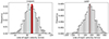 |
Fig. A.1. Distributions of line-of-sight velocities from Monte Carlo sampling for the two Milky Way satellite galaxies Crater II (left panel) and Leo V (right panel). The red bands give the range from sampling the measured line-of-sight velocities. The black histograms show the resulting line-of-sight velocities if errors are sampled in 6D Cartesian coordinates independently, ignoring their mutual correlations. |
Specifically, the upper panel in Fig. A.1 shows the results for Crater II, a satellite galaxy with relatively well constrained proper motions. Even in this case the incorrect sampling results in line-of-sight velocities deviating substantially from the actually measured value by tens of km/s. The situation is much worse for satellites with only poorly constrained proper motions (of which there are many), as demonstrated in the lower panel using Leo V as an example. In this case, the incorrect error sampling results in an extremely wide spread of line-of-sight velocities, some offset by hundreds of km/s from the actual measured value.
Appendix B: Scaled metric with equal-area bins
We here summarize our results after ensuring that the bins of the underlying 2D histograms in the metric’s spherical coordinates are of equal areas. To do this, we scale the original inclination angles β (that runs from 0 to π) to a new β′ = 0.5 π (1 − cos β). This ensures that the histograms have the same axis ranges as shown in Uzeirbegovic et al. (2024). We emphasize that even with equal areas, the shapes of the bins differ, with the bins closer to the poles being more elongated than those close to the equator of the coordinate system. This suggests that the scaled metric’s results remain sensitive to the orientation under which a satellite system is studied.
Figure B.1 shows the test on the effect of orientation, and confirms that an effect remains even for the scaled metric. The scaling improves the situation somewhat, with more of a correlation apparent between the rotated test systems. However, there is still substantial scatter in the inferred degree planarity for different orientations, making the metric unreliable.
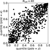 |
Fig. B.1. Quantiles for 1000 random isotropic distributions in two orientations, like Fig. 1 but now with bins of equal area. |
Figure B.2 repeats the test for prolate and oblate distributions. With the scaled metric the overall effect remains present, and in fact both prolate and oblate distributions now result in inferring increased degrees of planarity irrespective of the orientation. There does, however, remain some dependence on the orientation as can be seen be the lines for q = 0.5 and 2.0, as well as q = 0.67 and 1.5 effectively swapping placed between the upper and lower panels.
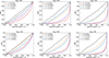 |
Fig. B.2. Distribution of quantiles in the scaled metric for systems with different degrees of flattening (q < 1.0, oblate) or elongation (q > 1.0, prolate) along the x-axis, and effect of the number of satellites on the inferred planarity of a distribution with intrinsic pro- or oblateness, using the scaled metric. |
Figure B.2 also shows that also in case of the scaled metric, the number of satellites in a system has an influence on the inferred degree of “planarity” if the systems are drawn from pro- or oblate distributions.
The scaled metric also returns increased degrees of “planarity” if satellite galaxies show clustering modeled as satellite pairs, similar but slightly more so than in the non-scaled case.
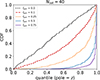 |
Fig. B.3. Distribution of quantiles in the scaled metric for isotropic distributions with different fractions of paired satellites. |
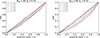 |
Fig. B.4. Effect of radial distribution and lopsidedness on the inferred planarity of a satellite system using the scaled metric. |
Figure B.4 shows that also in case of the scaled metric, the presence of a lopsided satellite distribution biases towards higher inferred degrees of “planarity”, and that also in this case the effect is stronger for more radially concentrated distributions. Furthermore, contrary to the non-scaled metric, the effect is now present in both considered orientations.
Appendix C: Radial distribution and lopsidedness
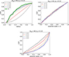 |
Fig. C.1. Effect of radial distribution and lopsidedness on the inferred planarity of a satellite system. The left panel plots the cumulative radial distribution of mock satellite systems (green: observed MW; black: fiducial distribution of Uzeirbegovic et al. 2024). The middle (right) panel shows the quantile distribution when the metric’s pole aligns with the z(x)-axis and thus perpendicular to (along) the offset. |
All Figures
|
Fig. 1. Quantiles for 1000 random isotropic distributions in two orientations rotated by 90°. No strong correlation is apparent, indicating that the output of the proposed ”planarity” metric is sensitive to the orientation of the satellite system under study. |
| In the text | |
|
Fig. 2. Distribution of quantiles for systems with different degrees of flattening (q < 1.0, oblate) or elongation (q > 1.0, prolate) along the x-axis. From left to right, the number of satellites per system is 20, 40, and 50, respectively. The upper panels orient the metric pole along the z-axis, and the lower panels orient it along the x-axis. |
| In the text | |
|
Fig. 3. Distribution of quantiles for isotropic distributions with different fractions of paired satellites. Even a mild degree of clustering results in a substantial increase in the high-quantile results. |
| In the text | |
|
Fig. A.1. Distributions of line-of-sight velocities from Monte Carlo sampling for the two Milky Way satellite galaxies Crater II (left panel) and Leo V (right panel). The red bands give the range from sampling the measured line-of-sight velocities. The black histograms show the resulting line-of-sight velocities if errors are sampled in 6D Cartesian coordinates independently, ignoring their mutual correlations. |
| In the text | |
|
Fig. B.1. Quantiles for 1000 random isotropic distributions in two orientations, like Fig. 1 but now with bins of equal area. |
| In the text | |
|
Fig. B.2. Distribution of quantiles in the scaled metric for systems with different degrees of flattening (q < 1.0, oblate) or elongation (q > 1.0, prolate) along the x-axis, and effect of the number of satellites on the inferred planarity of a distribution with intrinsic pro- or oblateness, using the scaled metric. |
| In the text | |
|
Fig. B.3. Distribution of quantiles in the scaled metric for isotropic distributions with different fractions of paired satellites. |
| In the text | |
|
Fig. B.4. Effect of radial distribution and lopsidedness on the inferred planarity of a satellite system using the scaled metric. |
| In the text | |
|
Fig. C.1. Effect of radial distribution and lopsidedness on the inferred planarity of a satellite system. The left panel plots the cumulative radial distribution of mock satellite systems (green: observed MW; black: fiducial distribution of Uzeirbegovic et al. 2024). The middle (right) panel shows the quantile distribution when the metric’s pole aligns with the z(x)-axis and thus perpendicular to (along) the offset. |
| In the text | |
Current usage metrics show cumulative count of Article Views (full-text article views including HTML views, PDF and ePub downloads, according to the available data) and Abstracts Views on Vision4Press platform.
Data correspond to usage on the plateform after 2015. The current usage metrics is available 48-96 hours after online publication and is updated daily on week days.
Initial download of the metrics may take a while.