| Issue |
A&A
Volume 694, February 2025
|
|
|---|---|---|
| Article Number | L3 | |
| Number of page(s) | 5 | |
| Section | Letters to the Editor | |
| DOI | https://doi.org/10.1051/0004-6361/202453411 | |
| Published online | 30 January 2025 | |
Letter to the Editor
Probing the low-energy particle content of blazar jets through MeV observations
1
INAF – Osservatorio Astronomico di Brera, Via E. Bianchi 46, I-23807 Merate, Italy
2
Dipartimento di Fisica, Universita‘ degli Studi di Genova, Via Dodecaneso 33, I-16146 Genova, Italy
3
Department of Astronomy, Yale University, PO Box 208101, New Haven, CT 06520-8101, USA
⋆ Corresponding author; fabrizio.tavecchio@inaf.it
Received:
12
December
2024
Accepted:
13
January
2025
Many of the blazars observed by Fermi actually have the peak of their time-averaged gamma-ray emission outside the ∼GeV Fermi energy range, at ∼MeV energies. The detailed shape of the emission spectrum around the ∼MeV peak places important constraints on acceleration and radiation mechanisms in the blazar jet and may not be the simple broken power law obtained by extrapolating from the observed X-ray and GeV gamma-ray spectra. In particular, state-of-the-art simulations of particle acceleration by shocks show that a significant fraction (possibly up to ≈90%) of the available energy may go into bulk quasi-thermal heating of the plasma crossing the shock rather than producing a nonthermal power-law tail. Other gentler but possibly more pervasive acceleration mechanisms, such as shear acceleration at the jet boundary, may result in a further build-up of the low-energy (γ ≲ 102) particle population in the jet. As already discussed for the case of gamma-ray bursts, the presence of a low-energy Maxwellian-like bump in the jet particle energy distribution can strongly affect the spectrum of the emitted radiation, for example producing an excess over the emission expected from a power-law extrapolation of a blazar’s GeV-TeV spectrum. We explore the potential detectability of the spectral component ascribable to a hot quasi-thermal population of electrons in the high-energy emission of flat-spectrum radio quasars (FSRQs). We show that for the typical physical parameters of FSRQs, the expected spectral signature is located at ∼MeV energies. For the brightest Fermi FSRQ sources, the presence of such a component will be constrained by the upcoming MeV Compton Spectrometer and Imager (COSI) satellite.
Key words: acceleration of particles / radiation mechanisms: non-thermal / shock waves / galaxies: jets
© The Authors 2025
 Open Access article, published by EDP Sciences, under the terms of the Creative Commons Attribution License (http://creativecommons.org/licenses/by/4.0), which permits unrestricted use, distribution, and reproduction in any medium, provided the original work is properly cited.
This article is published in open access under the Subscribe to Open model. Subscribe to A&A to support open access publication.
1. Introduction
Even after decades of effort, a detailed understanding of the physical processes responsible for the phenomenology of extragalactic relativistic jets still eludes us (see, e.g., Blandford et al. 2019). Basic questions related to jet dynamics, composition, and the role of magnetic fields await definitive answers. In particular, the nature of the mechanisms behind the dissipation of a jet’s bulk outflow energy, be it initially in the form of particles or Poynting flux, and the subsequent acceleration of particles to ultrarelativistic energies, as evidenced by the emission of some jets in the TeV band, remains a central problem (Sironi et al. 2015a; Matthews et al. 2020). The two main competitors are diffusive shock acceleration (DSA) and magnetic reconnection (MR). The two mechanisms are somewhat complementary, since DSA can efficiently work only for flows with low magnetization (σ), while MR naturally requires high σ (Sironi et al. 2015b). Highly magnetized jets seem to be the natural outcome of launching mechanisms involving the interplay of magnetic fields and BH rotation (e.g., Tchekhovskoy et al. 2011), thus favoring MR. However, models of the emission observed from blazars indicate low levels of magnetization in connection with the emitting region(s) (Sikora et al. 2005; Celotti & Ghisellini 2008; Tavecchio & Ghisellini 2016), potentially supporting DSA. Recent results in the polarimetric channel by the IXPE satellite also seem to point to shocks as the main actors in the acceleration (e.g., Liodakis et al. 2022), although other interpretations are possible, including Poynting-dominated jets (e.g., Bolis et al. 2024).
Particle-in-cell (PIC) simulations allow us to study in detail (albeit on small temporal and spatial scales) the acceleration processes, both in the case of DSA (e.g., Sironi & Spitkovsky 2011; Sironi et al. 2013; Crumley et al. 2019; Grošelj et al. 2024) and MR (e.g., Sironi & Spitkovsky 2014; Werner et al. 2018; Petropoulou et al. 2019; Werner & Uzdensky 2024). An established prediction for DSA is that, downstream of the shock, particles are heated and form a Maxwellian-like distribution, while only a small fraction (a few percent) of the particles, repeatedly crossing the shock, undergo DSA and form a power-law tail containing ≲10% of the energy dissipated at the shock (e.g., Spitkovsky 2008). This kind of distribution is also derived through simulations adopting the Monte Carlo approach (e.g., Summerlin & Baring 2012). The presence of the prominent thermal bump should imprint clear spectral signatures (e.g., Giannios & Spitkovsky 2009). The possible presence of these signatures has been in particular discussed for gamma-ray bursts (GRBs) (Eichler & Waxman 2005; Giannios & Spitkovsky 2009; Warren et al. 2018; Gao et al. 2024), but conclusive observational evidence for a thermal component is lacking. On the other hand, MR is expected to produce smooth power-law-like spectra (e.g., Petropoulou et al. 2019). In this case, therefore, we do not expect any narrow thermal components in the observed spectra.
Our aim is to explore the potential signatures of the electron thermal bump in the emission of flat-spectrum radio quasars (FSRQs). These are powerful blazars characterized by a dominant γ-ray component, probably produced through the inverse-Compton (IC) scattering of ambient radiation by relativistic leptons in the jet (e.g., Sikora et al. 1994; Ghisellini & Tavecchio 2009). A back-of-the-envelope calculation suggests that, for typical parameters, electrons belonging to the thermal component emit in the MeV band, which corresponds to the maximum of the high-energy component of FSRQs (e.g., Sikora et al. 2002; Ghisellini et al. 2017; Marcotulli et al. 2022)1. For several of these sources the observed flux in the MeV is within the reach of the upcoming Compton Spectrometer and Imager (COSI) satellite (Tomsick & COSI Collaboration 2022), which will give us the opportunity to test our scenario in the near future.
The paper is organized as follows. In Sect. 2 we present the model. In Sect. 3 we discuss the application to FSRQs and we present the results. Finally, in Sect. 4 we discuss the results and the observational prospects. Throughout the paper, the following cosmological parameters are assumed: H0 = 70 km s−1 Mpc−1, ΩM = 0.3, ΩΛ = 0.7.
2. The model
As an example calculation of what one might see if a significant fraction of a jet’s dissipated energy goes into bulk heating rather than nonthermal acceleration, we followed a standard one-zone approach (e.g., Maraschi & Tavecchio 2003). The region where the dissipation occurs was modeled as a sphere with (comoving) radius R, moving with bulk Lorentz factor Γ at an angle θv with respect to the line of sight2. The region is filled with a tangled magnetic field of strength B. Relativistic electrons emit through synchrotron and IC mechanisms. For the IC targets, we considered both internally produced synchrotron radiation (synchrotron self-Compton, SSC) and an external component (external Compton, EC) dominated by the quasar’s broad-line region (BLR). The BLR spectrum is a blackbody with (observer frame) temperature T and energy density Uext.
We did not attempt to model the dissipation/acceleration process. Rather, we assumed the rapid production (injection) of energetic electrons (or pairs), with an initial hybrid thermal plus nonthermal (power-law) energy distribution following Giannios & Spitkovsky (2009):
Here Ke is a normalization, and the thermal distribution is given by the Maxwell-Juttner distribution,
with K2 the modified Bessel function of the second kind. The parameter γth plays the role of an effective temperature T of the quasi-thermal distribution (γth = kT/mec2, with k the Boltzmann constant and me the electron rest mass), while γnth in Eq. (1) is the minimum Lorentz factor of the nonthermal tail, described as a power law with slope p with cutoff at γc (with γc ≫ γnth). These injected particles then cool and radiate.
The jet rest-frame total injected luminosity of this hybrid (thermal and nonthermal) electron population is
where V is the volume of the emitting region. It is useful to introduce the fraction of energy contained in the nonthermal tail with respect to the total energy:
We also define the average Lorentz factor of the electron population:
In the standard internal shock model the energy of the electrons in the post-shock region comes from the randomization of the bulk kinetic flux of the incoming protons. It is customary to define the parameter ϵe as the fraction of the energy available from the shock that is conveyed to nonthermal electrons (e.g., Sari et al. 1998). In our case this can be expressed as
where Γu is the Lorentz factor of the upstream fluid in the downstream frame, mp is the proton mass, and ṅp is the number flux of the protons (as measured in the downstream frame). Using the parameters introduced above it is possible to express ϵe as
Here we define the multiplicity η± = ṅe/ṅp, where ṅe = ∫Q(γ)dγ is the total injection rate of the electrons (both thermal and nonthermal). In a normal ep plasma, η± = 1. We also explore the case of a pair-enriched jet, for which η± > 1 (e.g., Sikora & Madejski 2000). In this case, protons share their energy with more than one lepton, causing ⟨γ⟩ to decrease for constant δ and ϵe (see Eq. (7)).
The injected energy distribution, Eq. (1), is used to calculate the electron energy distribution (EED) reached by the electrons after a light crossing time of the emission region, N(γ), with the standard continuity equation (e.g., Chiaberge & Ghisellini 1999):
![$$ \begin{aligned} \frac{\partial N(\gamma ,t)}{\partial t}=\frac{\partial }{\partial \gamma }\left[ \dot{\gamma } \, N(\gamma ,t)\right] + Q(\gamma ), \end{aligned} $$](/articles/aa/full_html/2025/02/aa53411-24/aa53411-24-eq8.gif)
where  is the energy-dependent radiative cooling rate (including synchrotron and IC emission) of electrons with Lorentz factor γ. For simplicity, we neglect the adiabatic cooling of the particles and the escape from the source. Equation (8) is solved numerically using the robust implicit method of Chang & Cooper (1970) to find the EED at time tem = R/c, for which we calculate the resulting emission (see, e.g., Ghisellini & Tavecchio 2009).
3. Fixing parameters
Since we intend to explore the effects of the complex EED on the spectral energy distribution (SED) of FSRQ, we assume benchmark values for the physical parameters of the blazar emission region inspired by modeling of FSRQs (e.g., Tavecchio et al. 2000; Ghisellini et al. 2010). We assume R = 5 × 1016 cm, B = 1.6 G, Γ = 20, θv = 3.7 deg (which combine to give a Doppler factor D = 15). For the external radiation we assume that the dominant radiation field is that associated with the BLR, approximated (in the source rest frame) as a blackbody peaking at νext = 2 × 10¹⁵ Hz (see the discussion in Tavecchio & Ghisellini 2008) with energy density Uext = 2.5 × 10⁻² erg cm−3 (e.g., Ghisellini & Tavecchio 2008). We further assume that the source is located at the typical redshift z = 2. In addition to the main physical quantities related to the emission region, our model depends on the parameters of the injected EED, Q(γ), which are uniquely fixed once δ, ⟨γ⟩, Le, p, and γc are specified.
A possible scenario for the origin of the shock at which electrons are heated and subsequently accelerated to high energies is that invoking the interaction of different portions of the flow characterized by different speed (internal shocks; e.g., Spada et al. 2001). In this case we expect a mildly relativistic shock, with Γu ∼ 1.5 − 2. These shocks can efficiently accelerate particles only for low magnetization of the plasma (Sironi et al. 2015b). FSRQ jets at the distance where the observed radiation is produced is expected to have a low magnetization (e.g., Sikora et al. 2005; Celotti & Ghisellini 2008). In these conditions we can rely on the results of Crumley et al. (2019) who report the analysis of PIC simulations for subluminal, high Mach number, mildly relativistic (Γu = 1.7) weakly magnetized jets. The simulations show the development of a thermal component with average Lorentz factor around ⟨γ⟩≈300, and of a nonthermal power law with slope 2.2–2.3 containing a small fraction of the shock energy, ϵe ≈ 10−3. However this last result could depend on the detailed configuration (i.e., inclination of the magnetic field and magnetization). PIC simulations of weakly magnetized, relativistic (Γu > 3) shocks show that the fraction of energy conveyed to nonthermal electrons can be much larger than that estimated in the mildly relativistic case, on the order of ϵe ≈ 10−1 (Sironi & Spitkovsky 2011). These conditions could apply to FSRQs if the acceleration occurs at a stationary oblique recollimation shock (e.g., Bodo & Tavecchio 2018; Zech & Lemoine 2021).
Given the large uncertainties related to the physical setup of the emission region and the physical parameters related to the acceleration process, for clarity in the following we consider a benchmark model (hereafter model A) with fixed δ = 0.15, ⟨γ⟩ = 100, and p = 2.3. With these parameters ϵe ≃ 10−2 for an ep plasma, in line with the results of the simulations mentioned above. However, we also explore and discuss the effect of different values of the parameters on the resulting spectrum. In all models we fix γc = 8 × 10⁴. The value of γc is relatively unimportant (as long as γc ≫ 103) since the high-energy end of the EC component is mainly shaped by the effect of the KN cross section (Tavecchio & Ghisellini 2008).
4. Results
The strong radiative losses (dominated by EC) imply that the system is in a fast-cooling regime. The injected electrons belonging to the thermal bump quickly cool, forming a power law ∝γ−2 down to very low Lorentz factors (γ ≈ 2, see Fig. 1 for which we assume the parameters of model A; see Table 1). Therefore, the EED reached at tem = R/c is composed by this power law up to the peak of the relativistic Maxwellian, followed by a rapid decline in correspondence with the exponential part of the thermal peak and, finally, by the (cooled) nonthermal power law (with slope p + 1) above γnth up to γc.
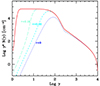 |
Fig. 1. Electron energy distribution in the emission region calculated at different times (given in units of the light crossing time, R/c) with the parameters used for model A. The equilibrium distribution comprises a cooled low-energy tail N(γ)∝γ−2, the high-energy tail (rapidly decreasing as a function of energy) of the thermal Maxwellian (which has the peak at γ ≃ 100), and the high-energy nonthermal power law with slope p + 1 (with p = 2.3 the slope of the injected power law) up to the cutoff at γc. |
The shape of the EED translates into a complex EC spectrum, with the notable presence of a bump produced by the thermal electrons belonging to the Maxwellian (see Fig. 2). The expected observed energy of the peak can be easily estimated, since Ep, obs ≈ hνextγp2ΓD/(1 + z), where γp ≈ 80 is the Lorentz factor at the peak of the Maxwellian. We therefore find Ep, obs ≃ 5 MeV.
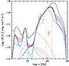 |
Fig. 2. SED calculated with the model described in the text. The colors indicate the following: model A (red), B (blue), C (light blue), D (green), and E (violet). The dash-dotted light green line shows the contribution from the accretion disk. We also report the contribution from the synchrotron (dotted), SSC (long-dashed), and EC (short-dashed). The vertical orange lines show the COSI energy band. For reference, in gray we also show the observational data points of the FSRQ 0836+710 (z = 2.1) from ASI-SSDC. |
The resulting observed SED is shown in Fig. 2 (red). The shape of the EED is clearly recognized in the EC bump, whose maximum corresponds to the emission of the electrons at the thermal peak. We note that in the synchrotron part of the SED the bump is partially visible, but the self-absorption of the spectrum, effectively cutting the emission at frequencies below 1012 Hz, strongly limits the effect. We also note that the imprint of the EED in the SSC component is smoothed. It is therefore clear that the details of the EED can be probed only in the MeV band. The extrapolation of the GeV spectrum to lower energies would clearly underpredict the flux in the MeV band. This MeV excess would be the “smoking gun” of the presence of a thermal component in the EED.
The other lines in Fig. 2 show the SED for different values of ⟨γ⟩ and δ (see Table 1). For the sake of comparison, we fix the luminosity emitted in the X-ray band (acting on Le) and we keep constant the parameters of the region (B, R, Γ, θv).
Parameters of the models.
Model B (blue lines) assumes a lower fraction of energy in the nonthermal tail (δ = 0.05) with respect to case A (δ = 0.15). While the thermal component is similar to case A, producing the same peak in the SED, the lower δ determines a lower nonthermal tail in the GeV band. This case is therefore characterized by a higher ratio between the MeV and the GeV fluxes, making the discrepancy between the extrapolated GeV flux and the actual MeV flux even more severe.
In model C (light blue) we assume a pair-rich jet with multiplicity η± = 2 (i.e., one e± pair every two protons). In this case the energy shared by protons to leptons must be distributed among more particles, decreasing the average Lorentz factors of the population. Correspondingly, the effective temperature of the thermal component decreases, shifting the peak of the EC bump to lower energies.
Model D is characterized by a larger ⟨γ⟩ = 300. The thermal peak shifts to high energies, exceeding 10 MeV. Due to the onset of the KN regime at energies above the EC peak, the transition between the thermal and the nonthermal part is smoother than in the other cases, making the identification of the two electron components more challenging than in previous cases. Finally, case E (violet) is for a very high δ = 0.3. In this case the power law increases its level with respect to the Maxwellian component, determining a less pronounced bump in the SED.
5. Discussion
Our results show that, within the large uncertainties related to the acceleration process and the composition of the jet, the peak of the thermal component is expected in the 0.1–10 MeV range, as observed for the most powerful FSRQ. Joint MeV and GeV observations can thus be exploited to trace the shape of the bump and potentially uncover the presence of the thermal component. We plan to perform dedicated simulations to assess the feasibility of observations with COSI (Tomsick & COSI Collaboration 2022).
In the alternative view invoking acceleration through MR, the anticipated spectrum is closely approximated by simple power laws (Petropoulou et al. 2019). Therefore, in principle, the absence of the thermal bump could support the MR scenario. However, one should keep in mind that the prominence of the thermal component with respect to the nonthermal power law, and therefore the possibility to disentangle the two corresponding spectral components, is strictly related to the parameter δ. Our results suggest that the two components could be relatively easily identified, even for cases with a large fraction of energy in nonthermal electrons, δ = 0.3. Recent PIC simulations (Grošelj et al. 2024) suggest that larger δ (> 0.5) can be reached in unmagnetized flows (e.g., associated with GRB afterglows), but it is unclear whether this result can be easily extended to (moderately) magnetized cases suitable for FSRQs.
The strong anticorrelation between the peak energy of the thermal component (and hence of the EC peak) and the pair content η± could already be used to rule out the case of a highly enriched plasma. A high multiplicity would imply a peak below the MeV band, in contrast with observations. Unfortunately, the uncertainties on the physical parameters associated with the acceleration (in particular ϵe) preclude definite conclusions. For instance, ϵe ∼ 0.1 (as derived for highly relativistic shocks) would allow η± ∼ 20 (e.g., as suggested by Sikora & Madejski 2000). In any case, a larger pair content seems to be excluded.
In this paper we studied the case of the most powerful FSRQs, for which the thermal component naturally falls in the MeV band. For other types of blazars the situation is less straightforward. Less powerful FSRQs display the EC peak at higher energies (100 MeV–1 GeV; e.g., Marcotulli et al. 2022). If related to the thermal bump, such high peak energies would imply correspondingly high electron temperature, possibly related to a larger dissipation parameter ϵe. We remark that in this case, the high-energy part of the EC component would be affected by KN effects that smooth the spectrum, making it difficult to identify the spectral structure; this effect is already visible in model D in Fig. 2). At even lower power, blazars of the BL Lac type (Low-peak synchrotron and High-peak synchrotron), display peaks above 10 GeV, which require electrons with γ ≳ 104 (e.g., Tavecchio et al. 2010), incompatible with thermal components from mildly relativistic shocks. In this case the thermal bump would instead appear in the low-energy part of the IC component. We note, however, that these sources produce high-energy radiation mainly through SSC, resulting in quite smooth spectra even for prominent thermal bumps (as also visible in Fig. 2).
An interesting issue concerns variability. One can expect that the physical parameters controlling the EED (δ, ⟨γ⟩) vary in time and determine the change of the position of the thermal bump and the relative level of thermal and nonthermal emission. The complex interplay between these effects could be in principle tracked by COSI (and Fermi) for the brightest FSRQs, with the MeV flux exceeding 10−10 erg cm−2 s−1. We plan to study the feasibility of this approach in a future publication.
Baring et al. (2017) performed a similar study, but they assumed a cold thermal component, whose emission peaks in the soft X-ray band.
Acknowledgments
We thank G. Ghisellini and E. Sobacchi for fruitful discussions. We acknowledge financial support from a INAF Theory Grant 2022 (PI F. Tavecchio). This work has been funded by the European Union-Next Generation EU, PRIN 2022 RFF M4C21.1 (2022C9TNNX). Part of this work is based on archival data provided by the Space Science Data Center-ASI.
References
- Baring, M. G., Böttcher, M., & Summerlin, E. J. 2017, MNRAS, 464, 4875 [CrossRef] [Google Scholar]
- Blandford, R., Meier, D., & Readhead, A. 2019, ARA&A, 57, 467 [NASA ADS] [CrossRef] [Google Scholar]
- Bodo, G., & Tavecchio, F. 2018, A&A, 609, A122 [NASA ADS] [CrossRef] [EDP Sciences] [Google Scholar]
- Bolis, F., Sobacchi, E., & Tavecchio, F. 2024, A&A, 690, A14 [NASA ADS] [CrossRef] [EDP Sciences] [Google Scholar]
- Celotti, A., & Ghisellini, G. 2008, MNRAS, 385, 283 [NASA ADS] [CrossRef] [Google Scholar]
- Chang, J. S., & Cooper, G. 1970, J. Comput. Phys., 6, 1 [Google Scholar]
- Chiaberge, M., & Ghisellini, G. 1999, MNRAS, 306, 551 [Google Scholar]
- Crumley, P., Caprioli, D., Markoff, S., & Spitkovsky, A. 2019, MNRAS, 485, 5105 [NASA ADS] [CrossRef] [Google Scholar]
- Eichler, D., & Waxman, E. 2005, ApJ, 627, 861 [NASA ADS] [CrossRef] [Google Scholar]
- Gao, H.-X., Geng, J.-J., Sun, T.-R., et al. 2024, ApJ, 971, 81 [NASA ADS] [CrossRef] [Google Scholar]
- Ghisellini, G., & Tavecchio, F. 2008, MNRAS, 387, 1669 [NASA ADS] [CrossRef] [Google Scholar]
- Ghisellini, G., & Tavecchio, F. 2009, MNRAS, 397, 985 [Google Scholar]
- Ghisellini, G., Tavecchio, F., Foschini, L., et al. 2010, MNRAS, 402, 497 [Google Scholar]
- Ghisellini, G., Righi, C., Costamante, L., & Tavecchio, F. 2017, MNRAS, 469, 255 [NASA ADS] [CrossRef] [Google Scholar]
- Giannios, D., & Spitkovsky, A. 2009, MNRAS, 400, 330 [NASA ADS] [CrossRef] [Google Scholar]
- Grošelj, D., Sironi, L., & Spitkovsky, A. 2024, ApJ, 963, L44 [CrossRef] [Google Scholar]
- Liodakis, I., Marscher, A. P., Agudo, I., et al. 2022, Nature, 611, 677 [CrossRef] [Google Scholar]
- Maraschi, L., & Tavecchio, F. 2003, ApJ, 593, 667 [Google Scholar]
- Marcotulli, L., Ajello, M., Urry, C. M., et al. 2022, ApJ, 940, 77 [NASA ADS] [CrossRef] [Google Scholar]
- Matthews, J. H., Bell, A. R., & Blundell, K. M. 2020, New Astron. Rev., 89, 101543 [CrossRef] [Google Scholar]
- Petropoulou, M., Sironi, L., Spitkovsky, A., & Giannios, D. 2019, ApJ, 880, 37 [Google Scholar]
- Sari, R., Piran, T., & Narayan, R. 1998, ApJ, 497, L17 [Google Scholar]
- Sikora, M., & Madejski, G. 2000, ApJ, 534, 109 [NASA ADS] [CrossRef] [Google Scholar]
- Sikora, M., Begelman, M. C., & Rees, M. J. 1994, ApJ, 421, 153 [Google Scholar]
- Sikora, M., Błażejowski, M., Moderski, R., & Madejski, G. M. 2002, ApJ, 577, 78 [NASA ADS] [CrossRef] [Google Scholar]
- Sikora, M., Begelman, M. C., Madejski, G. M., & Lasota, J.-P. 2005, ApJ, 625, 72 [NASA ADS] [CrossRef] [Google Scholar]
- Sironi, L., & Spitkovsky, A. 2011, ApJ, 726, 75 [NASA ADS] [CrossRef] [Google Scholar]
- Sironi, L., & Spitkovsky, A. 2014, ApJ, 783, L21 [NASA ADS] [CrossRef] [Google Scholar]
- Sironi, L., Spitkovsky, A., & Arons, J. 2013, ApJ, 771, 54 [Google Scholar]
- Sironi, L., Keshet, U., & Lemoine, M. 2015a, Space Sci. Rev., 191, 519 [CrossRef] [Google Scholar]
- Sironi, L., Petropoulou, M., & Giannios, D. 2015b, MNRAS, 450, 183 [Google Scholar]
- Spada, M., Ghisellini, G., Lazzati, D., & Celotti, A. 2001, MNRAS, 325, 1559 [NASA ADS] [CrossRef] [Google Scholar]
- Spitkovsky, A. 2008, ApJ, 682, L5 [NASA ADS] [CrossRef] [Google Scholar]
- Summerlin, E. J., & Baring, M. G. 2012, ApJ, 745, 63 [NASA ADS] [CrossRef] [Google Scholar]
- Tavecchio, F., & Ghisellini, G. 2008, MNRAS, 386, 945 [CrossRef] [Google Scholar]
- Tavecchio, F., & Ghisellini, G. 2016, MNRAS, 456, 2374 [Google Scholar]
- Tavecchio, F., Maraschi, L., Ghisellini, G., et al. 2000, ApJ, 543, 535 [Google Scholar]
- Tavecchio, F., Ghisellini, G., Ghirlanda, G., Foschini, L., & Maraschi, L. 2010, MNRAS, 401, 1570 [Google Scholar]
- Tchekhovskoy, A., Narayan, R., & McKinney, J. C. 2011, MNRAS, 418, L79 [NASA ADS] [CrossRef] [Google Scholar]
- Tomsick, J., & COSI Collaboration 2022, in 37th International Cosmic Ray Conference, 652 [Google Scholar]
- Warren, D. C., Barkov, M. V., Ito, H., Nagataki, S., & Laskar, T. 2018, MNRAS, 480, 4060 [NASA ADS] [CrossRef] [Google Scholar]
- Werner, G. R., & Uzdensky, D. A. 2024, ApJ, 964, L21 [NASA ADS] [CrossRef] [Google Scholar]
- Werner, G. R., Uzdensky, D. A., Begelman, M. C., Cerutti, B., & Nalewajko, K. 2018, MNRAS, 473, 4840 [Google Scholar]
- Zech, A., & Lemoine, M. 2021, A&A, 654, A96 [NASA ADS] [CrossRef] [EDP Sciences] [Google Scholar]
All Tables
All Figures
|
Fig. 1. Electron energy distribution in the emission region calculated at different times (given in units of the light crossing time, R/c) with the parameters used for model A. The equilibrium distribution comprises a cooled low-energy tail N(γ)∝γ−2, the high-energy tail (rapidly decreasing as a function of energy) of the thermal Maxwellian (which has the peak at γ ≃ 100), and the high-energy nonthermal power law with slope p + 1 (with p = 2.3 the slope of the injected power law) up to the cutoff at γc. |
| In the text | |
|
Fig. 2. SED calculated with the model described in the text. The colors indicate the following: model A (red), B (blue), C (light blue), D (green), and E (violet). The dash-dotted light green line shows the contribution from the accretion disk. We also report the contribution from the synchrotron (dotted), SSC (long-dashed), and EC (short-dashed). The vertical orange lines show the COSI energy band. For reference, in gray we also show the observational data points of the FSRQ 0836+710 (z = 2.1) from ASI-SSDC. |
| In the text | |
Current usage metrics show cumulative count of Article Views (full-text article views including HTML views, PDF and ePub downloads, according to the available data) and Abstracts Views on Vision4Press platform.
Data correspond to usage on the plateform after 2015. The current usage metrics is available 48-96 hours after online publication and is updated daily on week days.
Initial download of the metrics may take a while.