| Issue |
A&A
Volume 694, February 2025
|
|
|---|---|---|
| Article Number | A318 | |
| Number of page(s) | 12 | |
| Section | Planets, planetary systems, and small bodies | |
| DOI | https://doi.org/10.1051/0004-6361/202452394 | |
| Published online | 24 February 2025 | |
Terrestrial planet formation during giant planet formation and giant planet migration
I. The first five million years
1
Konkoly Observatory, HUN-REN CSFK, MTA Centre of Excellence ;
Konkoly Thege Miklos St. 15–17,
1121
Budapest,
Hungary
2
Centre for Planetary Habitability (PHAB), University of Oslo,
Sem Saelands Vei 2A,
0371
Oslo,
Norway
★ Corresponding author; This email address is being protected from spambots. You need JavaScript enabled to view it.
Received:
27
September
2024
Accepted:
13
January
2025
Abstract
Context. Terrestrial planet formation (TPF) is a difficult problem that has vexed researchers for decades. Numerical models are only partially successful at reproducing the orbital architecture of the inner planets, but have generally not considered the effect of the growth of the giant planets. Cosmochemical experiments suggest that the nucleosynthetic isotopic composition of bodies from beyond Jupiter is different from that of the inner Solar System. This difference could have implications for the composition of the terrestrial planets.
Aims. I aim to compute how much material from the formation region of the gas giants ends up being implanted in the inner Solar System due to gas drag from the protoplanetary disc, how this implantation alters the feedstocks of the terrestrial planets, and whether this implantation scenario is consistent with predictions from cosmochemistry.
Methods. I dynamically model TPF as the gas giants Jupiter and Saturn are growing using the Graphics Processing Unit (GPU) software Gravitational ENcounters with GPU Acceleration (GENGA). The evolution of the masses, radii, and orbital elements of the gas giants are precomputed and read and interpolated within GENGA. The terrestrial planets are formed by planetesimal accretion from tens of thousands of self-gravitating planetesimals spread between 0.5 au and 8.5 au. The total mass of the inner planetesimal disc and outer disc are typically 2 and 3 Earth masses (M⊕) respectively, and the composition of the planetesimals changes from non-carbonaceous-like to carbonaceous-like at a prescribed distance, ranging from 2 au to 5 au.
Results. Here, I report on the first 5 million years of evolution. At this time approximately 20% of the mass of planetesimals in the Jupiter-Saturn region is implanted in the inner Solar System, which could be more than the cosmochemical models predict; this amount can be reduced by reducing the total mass of the outer planetesimal disc, and the results suggest a mass of 1 M⊕ could suffice. The mass-weighted fraction of outer Solar System material implanted in the inner Solar System shows a flat or bimodal distribution beyond 0.7 au, with an occasional peak near 0.9 au. The planetesimals that remain in the inner Solar System have a mixed composition, which could have implications for late accretion.
Conclusions. The growing gas giants scattered the planetesimals in their vicinity into the inner Solar System, which changed the isotopic composition of the terrestrial planets. The inner planetesimal disc may not have extended much farther than 2 au, otherwise embryos do not grow fast enough to produce Mars analogues. This could mean that the region of the current asteroid belt never contained much mass to begin with. The implantation scenario could also explain the existence of active asteroids in the main belt.
Key words: planets and satellites: dynamical evolution and stability / planets and satellites: formation / planets and satellites: terrestrial planets
© The Authors 2025
 Open Access article, published by EDP Sciences, under the terms of the Creative Commons Attribution License (https://creativecommons.org/licenses/by/4.0), which permits unrestricted use, distribution, and reproduction in any medium, provided the original work is properly cited.
This article is published in open access under the Subscribe to Open model. This email address is being protected from spambots. You need JavaScript enabled to view it. to support open access publication.
1 Introduction
Dynamical modelling of terrestrial planet formation (TPF) has a long history, dating back to the early works of Wetherill & Stewart (1989), and the state-of-the-art N-body simulations of Kokubo & Ida (1995, 1996, 1998) using the GRAvity PipE (GRAPE) specialised hardware (Ito et al. 1990). To date, there is an overabundance of dynamical models of TPF in existence. Past and present dynamical models either rely on planetesimal accretion, or on pebble accretion, which is a mode of planetary growth developed by Ormel & Klahr (2010) and Lambrechts & Johansen (2012).
The first model that relied on planetesimal accretion to grain traction is dubbed the classical model (Chambers 2001; Raymond et al. 2006, 2009; O’Brien et al. 2006; Walsh & Levison 2019; Woo et al. 2021), wherein the giant planets were assumed to have fully formed and reside on their current orbits. The terrestrial planets formed by planetesimal accretion from a planetesimal disc roughly situated between 0.5 au and 4 au with a surface density slope similar to the minimum-mass solar nebula (Hayashi 1981). A variation on this model assumes Jupiter and Saturn on circular orbits (Raymond et al. 2009). The growth of the planets roughly proceeded as follows: as the planets grew and the planetesimals were depleted, the initial runaway mode of growth changed to an oligarchic growth mode (Kokubo & Ida 1998), wherein a convoy of lunar to Mars mass planetary embryos at their isolation mass (Lissauer 1987) stirred up and accreted the remaining planetesimals, while the embryos remained roughly evenly spaced apart. The planetesimals could provide dynamical friction to the embryos, keeping their eccentricities and inclinations low (O’Brien et al. 2006). Eventually this configuration became dynamically unstable, and the embryos underwent a phase of mutual collisions (dubbed the giant impact phase) and they merged to form Venus and Earth (Chambers 2001).
Unfortunately, the classical model suffers from the ‘small Mars’ problem, in which the mass of formed planets near the current orbit of Mars are systematically too great (Chambers 2001; O’Brien et al. 2006; Raymond et al. 2006, 2009; Walsh & Levison 2019; Woo et al. 2021). Proposed solutions for this problem are: limiting the width of the initial planetesimal disc in the annulus model (Hansen 2009; Izidoro et al. 2022), invoking the migration of the giant planets to truncate the planetesimal disc with the Grand Tack model (Walsh et al. 2011), lowering the planetesimal surface density beyond Mars with the depleted disc model (Izidoro et al. 2014; Mah & Brasser 2021), steepening the surface density slope of the planetesimal disc (Izidoro et al. 2015), and invoking an early dynamical instability of the giant planets to stir up the inner Solar System (Clement et al. 2018) and Clement et al. (2019). Each of these models has their pros and cons in terms of reproducing the mass-semi-major axis distribution, angular momentum deficit (AMD; Laskar 1997), growth rates of Earth and Venus (Kleine et al. 2009; Rudge et al. 2010), and timing of the Moon-forming event (Jacobson et al. 2014). A review of TPF models can be found in Morbidelli et al. (2012), and a brief discussion of each model’s outcomes are given in Lammer et al. (2021).
The great diversity of planetesimal accretion models in existence betrays the fact that further progress relying on simplified dynamical models running on single central processing unit (CPU) cores is limited. Simulations beginning with a few thousand planetesimals and planetary embryos take a few months to complete, and higher planetesimal numbers are prohibitively expensive in terms of required computing resources, unless certain approximations are made (e.g. Gaburov et al. 2010; Bédorf et al. 2012b). This has led to the creation of the Lagrangian Integrator for Planetary Accretion and Dynamics (LIPAD) (Levison et al. 2012), which uses tracer particles to follow the collisional, accretional, and dynamical evolution of a large number of small planetesimals through the entire growth process of becoming planets. Collisions are treated in a statistical manner and the code is parallelised (i.e. it uses multiple CPU cores). An example study of TPF with LIPAD indicates that the small Mars problem could have partially been an artefact of the numerical limitations of using a single CPU core, the initial conditions used in earlier models, as well as embryo growth times exceeding five million years (Myr) beyond 1.5 au (Walsh & Levison 2019). As such, LIPAD offers promising solutions to study TPF, but to this author’s knowledge it is not open source so that its adoption and the verification of its results remain limited.
The popularity of computing on graphics cards, called graphical processing units (GPUs), and the availability of hardware and dedicated N-body codes that run on them, is increasing. Examples such as Bonsai (Bédorf et al. 2012a) and Gravitational ENcounters with GPU Acceleration (GENGA) (Grimm & Stadel 2014; Grimm et al. 2022), opened up additional pathways of exploration beyond LIPAD; it became possible to simulate tens of thousands of self-gravitating planetesimals on one GPU card, and thereby to track the growth of Mars from planetesimal accretion (Woo et al. 2021). With GPU computing the small Mars problem did not entirely disappear, indicating that treating collisions better than just mergers may have a strong effect on the outcome (Walsh & Levison 2019). However, these technological developments by themselves do not solve all the problems that the existing dynamical models have. What is worse, and therefore important, is that understanding TPF requires more than statistically reproducing the masses and orbital properties of the terrestrial planets because they also have different compositions. A good model of TPF should be able to at least reproduce these differences.
Apart from the great variety of outcomes resulting from dynamical studies, problems also arise from (mass-independent) isotopic anomalies measured in samples from the Earth, Moon, Mars, Vesta, and various other meteorite classes. These anomalies consistently indicate that intrinsic compositional differences existed in various regions of the Sun’s protoplanetary disc (Warren 2011). Experimental analyses indicate that the isotopic composition of Mars is consistently different from that of the Earth in terms of nucleosynthetic anomalies in Ti, Cr, Fe, Zn, Mo and O (see review by Mezger et al. 2020). When correlating these isotopic anomalies of different elements in the planets and meteorites against each other, two major groupings emerge: a carbonaceous or Jovian group, purportedly from the outer Solar System, and a non-carbonaceous or terrestrial group, purportedly from the inner region (e.g. Warren 2011; Brasser & Mojzsis 2020). In other words, the isotopic composition of Solar System samples show a dichotomy (e.g. Warren 2011; Mezger et al. 2020; Kruijer et al. 2020). There is debate whether these differences arose from a compositional gradient that existed in the Sun’s protoplanetary disc (Yamakawa et al. 2010). Monte Carlo models that mix various chondrites as isotopic proxies for the building blocks of the Earth and Mars show that these planets formed primarily from terrestrial group material (Fitoussi et al. 2016; Dauphas 2017; Dauphas et al. 2024). This reservoir is the likely source of Earth’s water (Piani et al. 2020). These mixing models also consistently indicate that the isotopic compositions of the Earth and Mars require them both to have accreted a few weight percent (wt.%) of Jovian group material (Fitoussi et al. 2016; Dauphas 2017; Dauphas et al. 2024). Despite the quality of the measurements that provide the input for these mixing models and their numerical robustness, their conclusions are difficult to explain dynamically: the impact probability of Jovian group material with the terrestrial planets is extremely low if it arrived directly from beyond Jupiter after the gas disc dissipated (Brasser et al. 2020). This probability is greatly enhanced if this material was delivered during the gas phase with pebble accretion, although that scenario has its own set of problems (Mah et al. 2022; Morbidelli et al. 2025).
In addition to their different nucleosynthetic isotopic compositions, the Earth and Mars also have disparate growth times. Mars is thought to have almost fully formed within 5 Myr after the formation of the Solar System (Dauphas & Pourmand 2011; Tang & Dauphas 2014), in other words, while the protosolar disc was still there (Wang et al. 2017; Weiss et al. 2021). The giant planets, by their nature, must also have formed while the protosolar disc was there, and their N isotopes indicate their gaseous envelopes are likely accreted from the protosolar disc (Marty et al. 2011; Füri & Marty 2015). From the Hf-W dating of iron meteorites and arguing that Jupiter is responsible for the dichotomy, Kruijer et al. (2017) infer that Jupiter formed in 1–2 Myr after the formation of the Solar System, contemporary with Mars. In contrast, the Earth took much longer, from 10 to 50 Myr (e.g. Yin et al. 2002; Kleine et al. 2009; Yu & Jacobsen 2011), culminating in the Moon-forming event, whose timing is still debated – see the discussion in Thiemens et al. (2019); Kruijer et al. (2021); Thiemens et al. (2021).
The simultaneous growth of Mars and Jupiter implies that TPF should no longer be studied in isolation, and that the growth of the gas giants should be included in dynamical models, or at least considered. The growing gas giants could have a profound effect on the composition of the inner Solar System because they scattered nearby planetesimals into the terrestrial region where gas drag circularised their orbits (Raymond & Izidoro 2017a). The recent analyses of samples from asteroid (162173) Ryugu returned by JAXA’s Hayabusa2 mission suggest that Ryugu and CI chondrites formed in the same region of the protoplanetary disc (e.g. Yokoyama et al. 2022), probably far away from the Sun. This has led Nesvorný et al. (2024) to perform a similar study to that of Raymond & Izidoro (2017a) wherein they numerically quantified the implantation amount of CI-like material in the Uranus-Neptune region of the protoplanetary disc to the main asteroid belt. Potential further evidence for the implantation scenario comes from purported early volatile accretion onto the angrite parent body (Sarafian et al. 2014, 2017) (cf. Rider-Stokes et al. 2024), while the composition of the asteroid belt implies either mixing and/or the implantation of materials (Walsh et al. 2011; Deienno et al. 2022), or at least the existence of a compositional gradient (DeMeo & Carry 2014).
The main motivation for this study is cosmochemical: I want to build a model of TPF that accounts for the compositional diversity of Earth, Mars and Vesta. The implantation model of Raymond & Izidoro (2017a) has the potential to explain these features. The author opines that this scenario can explain the small amount of Jovian material accreted by the terrestrial planets rather than relying on pebble accretion (cf. Schiller et al. 2018, 2020), and to further account for the isotopic differences between the Earth and Mars, as well as explain the composition of (162173) Ryugu (Nesvorný et al. 2024). An additional motivation is provided by the idea that the CO, CV and CM carbonaceous chondrites could have formed in the main asteroid belt rather than beyond Jupiter (Marrocchi et al. 2018), for which dynamical models would predict a higher incorporation efficiency than if these formed beyond Jupiter. Here I take the work of Raymond & Izidoro (2017a) to the next step. Not only do I trace how outer Solar System material finds its way into the inner Solar System, and what the implantation efficiency is, but I also track how (most of) this material is incorporated into the growing terrestrial planets. Recent studies place some model constraints on the growth times of Jupiter and Saturn when these for together (Lau et al. 2024; Raorane et al. 2024), so that the time has come for an in-depth study of how giant planet formation affects TPF. Regrettably, Raorane et al. (2024) had difficulty forming ice giant analogues, so that, unlike Nesvorný et al. (2024), at present I do not address the implantation of distant (>10 au) material into the main asteroid belt.
The argument can be made that the dichotomy came to exist before the formation of Jupiter (Brasser & Mojzsis 2020) (cf. Kruijer et al. 2017) and that the physical separation must have occurred at or beyond where Jupiter is today. However, if it is indeed possible that the CO, CV and CM carbonaceous chondrites could have formed in the main asteroid belt rather than beyond Jupiter, then this idea warrants investigation. As such, here I also explore the effect of having the boundary between terrestrial and Jovian group material be closer to the Sun than at 5 au.
This paper is part of a series of manuscripts detailing the implantation process, and how much Jovian material could end up incorporated into the terrestrial planets and the main asteroid belt as a function of initial conditions. Here I focus on the first five Myr of evolution, when the protosolar disc was still around. Future publications will reveal its long-term evolution.
2 Methods
2.1 Growth of the gas giants
The first thing my model requires is to have a prescription for the growth of the giant planets. Raymond & Izidoro (2017a) began with Jupiter and Saturn as planetary cores with a mass of three Earth masses (M⊕) each, and then grew their masses to their current values on a timescale of 0.1 million years, although faster and slower growth timescales were also tested. Here I want to have the growth timescales of Jupiter and Saturn match that of dynamical simulations of pebble accretion, but also not be too different from that adopted by Raymond & Izidoro (2017a) for easier comparison.
Following Brasser & Mojzsis (2020) and guided by the extensive simulations of giant planet formation in the Solar System with pebble accretion by Lau et al. (2024) and Raorane et al. (2024), I generated growth tracks of the giant planets using the N-body integrator Symplectic Massive Body Algorithm (SyMBA; Duncan et al. 1998), which was modified to include the effects of pebble accretion, gas accretion and damping forces from the gas disc (Matsumura et al. 2021). These highly simplified simulations started with two Ceres-mass planetesimals at 5.6 au and 7.5 au which were subjected to a flux of pebbles; I could have chosen larger initial masses, but I found that these initial values satisfied the growth rates from Raymond & Izidoro (2017a) and Raorane et al. (2024) because the initial growth is slow, causing a slight delay until there is gas envelope accretion of the Jupiter analogue. The disc parameters, pebble flux and temporal disc evolution were the same as those in Raorane et al. (2024): the initial mass of the protoplanetary disc was 0.05 solar masses (M⊕), the diffusion timescale of the gas was set to 0.5 million years and the slope of the temperature gradient in this region of the disc was that of the irradiated regime, that is |d ln T/d ln r| = 3/7 (Ida et al. 2016). The temporal mass accretion onto the star and the pebble mass flux are given by
 (1)
(1)
where I have substituted nominal disc and pebble radius parameters (Matsumura et al. 2021; Lau et al. 2024; Raorane et al. 2024). Here αacc is the accretion viscosity and tpff is the pebble formation time (Ida et al. 2016). The pebble accretion prescription and disc model of Ida et al. (2016) was used assuming perfect accretion efficiency. With these parameters the pebble radii at the locations of Jupiter and Saturn were rpeb = 18.3 cm and rpeb = 12.3 cm while their Stokes numbers were 𝒮 = 0.45 and 𝒮 = 0.40.
Gas envelope accretion was computed as described in Raorane et al. (2024), where I used the same input parameters as that study. In short, the gas envelope mass evolved as (Ida et al. 2018)
![Mathematical equation: ${{d{M_{{\rm{env}}}}} \over {dt}} = \min \left[ {{{{M_{{\rm{core}}}}} \over {{\tau _g}}},{{\dot M}_*},{f_{{\rm{gap}}}}{{\dot M}_*}} \right],$](/articles/aa/full_html/2025/02/aa52394-24/aa52394-24-eq2.png) (2)
(2)
where ƒgap is a reduction factor due to gap opening of the growing planet (Ida et al. 2018), which is given by
 (3)
(3)
where mp is the mass of the planet, h is the reduced gas scale height, and where τɡ is the gas accretion timescale. The last quantity is given by
 (4)
(4)
where Mcore is the core mass and κgr is the grain opacity (Ikoma et al. 2000); for this study I used an opacity of 1 cm2 g−1. The factor K is related to gap opening and is given by (Kanagawa et al. 2018)
 (5)
(5)
where αturb represents the strength of the local disc turbulence, which I set to αturb = 10−4. Gap opening becomes important when K = 25.
The time step in the simulation was 0.1 yr and the simulations were run for 5 Myr. I switched off the effect of planetary migration to mimic a purported disc pressure maximum at 5 au (Brasser & Mojzsis 2020) and to not have the growing gas giants encounter each other, or to migrate all the way to terrestrial planet region. The outcome of this setup seems inconsistent with the results from Raorane et al. (2024), wherein massive gas giants frequently experienced mutual encounters and Jupiter analogues were on average farther away than Saturn analogues, but the purpose of this study is to establish the implantation efficiency and how Jovian material was incorporated into the terrestrial planets.
The growth time of Jupiter calculated here is similar to what was used by Raymond & Izidoro (2017a), and although it is fast it is still consistent with that reported in Raorane et al. (2024). A follow-up study using a slower growth of Jupiter is in progress.
The mass evolution of both planets is shown in Fig. 1. Both planets grow from pebble accretion until approximately 6 M⊕, after which gas accretion sets in Matsumura et al. (202l). The planet’s masses were truncated to their current values. The growth rate of Jupiter from when it reaches 3 M⊕ to its current value is similar to that employed by Raymond & Izidoro (2017a), while in my simulation Saturn’s growth is much slower. The growth rate of Jupiter calculated here is much faster but still statistically consistent with that found in Raorane et al. (2024), while the growth rate of Saturn is mostly consistent with that study. Although the growth rate of Jupiter is fast, the initial simulation time t = 0 is somewhat arbitrary when compared to the absolute age of the Solar System and the meteorite record, with a probable window comparable to the growth of the non-carbonaceous iron meteorites, that is ~0.5 million years (Kruijer et al. 2014). From these growth tracks I extracted orbital elements, masses, and radii of the gas giants. The mass-radius relationship for planetesimals and planet cores that I used here is given by Seager et al. (2007). The following equation was used for cold terrestrial planets mp < 5 M⊕ of all compositions:
 (6)
(6)
where mp and R are the mass and radius of the planet, and where k1 = −0.2095, k2 = 0.0804, and k3 = −0.3940. For planets more massive than 5 M⊕ I used the prescription R = 1.65(mp/5 M⊕)1/2 R⊕ from Weiss & Marcy (2014). Simulations wherein the gas giants have enhanced envelopes due to accretional heat loss are under investigation. Both gas giants became slightly eccentric due to their mass growth, which altered the centre of mass of the system, with their mutual perturbations also inducing some finite value of eccentricity.
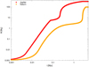 |
Fig. 1 Growth of the masses of Jupiter and Saturn as a function of time adopted in this study. |
2.2 GPU simulations of TPF with growing gas giants
Next, I ran GPU N-body simulations using GENGA of a population of planetesimals in the presence of gas from the proto-planetary disc. This population was subjected to the growing Jupiter and Saturn. At present GENGA does not have pebble accretion implemented, so that the gravitational effect of the growing gas giants on the inner Solar System has to be approximated. GENGA can read and interpolate masses, radii, and orbital elements of bodies from a table, so I made use of that here. Specifically, I in read the masses, radii, semi-major axes, eccentricities, and argument of perihelion of the gas giants every 100 yr. The gas giants’ mutual inclinations were zero, and their nodes were fixed. With the amount of High Performance Computing (HPC) time I had available I was able to run eight sets of eight simulations. The simulation sets differed in their initial conditions in total planetesimal mass and planetesimal number. In Table 1 I list the different initial conditions of the sets of simulations. Each individual simulation started with 19k to 47k self-gravitating planetesimals situated between 0.5 au and 8.5 au, and two Ceres-sized bodies at 5.6 au and 7.5 au that were artificially grown to become Jupiter and Saturn. Planetesimals usually had a radius between 300 and 600 km and were fully interacting, they were uniformly randomly distributed in semimajor axis in each annulus (inner and outer), they had uniformly random eccentricities ≤0.001,inclinations ≤0.5º, and uniformly randomised other angles. The mass of the planetesimal disc that is a proxy for terrestrial material is listed as minner and typically consists of 8k to 10k planetesimals; similarly the mass of the outer planetesimal disc located up to 8.5 au is denoted mouter and consists of 8k to 37k planetesimals. The distance at which I assumed the composition of the bodies to change from terrestrial type to Jovian type is listed as ‘Change’; Raymond & Izidoro (2017a) initially assumed that a change in composition occurred at 4 au. This is a sharp transition between the two groups of material, but this approach makes tracking the evolution of material in each group much easier than when the gradient is more gradual. If there is an empty region, to mimic an initially empty asteroid belt (Raymond & Izidoro 2017b; Deienno et al. 2024) or planetesimal formation in a ring (Hansen 2009; Izidoro et al. 2022), the inner and outer edges are specified in ‘Gap’.
Simulations were run for 5 Myr with a time step of 0.01 yr; the remaining evolution is discussed in a forthcoming publication. The surface density of the protoplanetary disc declined exponentially with an e-folding time of 1 Myr; its initial value was 1700 g cm−2 at 1 au with an inner edge of 0.4 au, and the surface density declined with distance as r−1. No migration was imposed in order to avoid a pileup of embryos in the Mercury region (Woo et al. 2021), and because there could have been a pressure maximum near Venus that could have impeded this migration (Woo et al. 2023; Chambers 2023). GENGA has the option to only apply the gas forces and torques to bodies less massive than a threshold mass, dubbed mGiant. In my simulations most of the planetesimals had an initial mass comparable to the seeds of Jupiter and Saturn. The latter two bodies must not be subjected to the gas forces because it caused errors in the interpolation of their growth tracks, hence mGiant must have been smaller than their initial masses. To model this accurately I would have had to start and stop the simulations and adjust mGiant at specific times, which would have caused strange behaviour in the migration. As such, I opted for simplicity and had none of the bodies be subjected to migration. Planetesimals with mass m < mGiant experienced both gas drag and eccentricity and inclination damping from the gas disc as implemented in GENGA (Grimm et al. 2022) based on the prescription of Morishima et al. (2010); further details of their prescriptions can be found in Woo et al. (2021). The avoidance of a pileup of embryos in the Mercury region is addressed by the works of Clement et al. (2021b); Clement & Chambers (2021); Clement et al. (2021a) and in Woo et al. (2023). In future studies I address this problem in a similar manner. Bodies were removed closer than 0.3 au or farther than 300 au from the Sun, or when there was a collision. Perfect mergers are assumed whenever there was a collision between bodies.
Simulation parameters.
3 Results
In this work I focus on how the implantation of planetesimals from the Jovian group affects the bulk composition of the terrestrial planets, beginning with planetary embryos here and going all the way to the final terrestrial planets in a subsequent publication. As such, I do not describe the detailed dynamics of the swarm of planetesimals because it is very similar to that of Woo et al. (2021) and that of Raymond & Izidoro (2017a). I refer to those works for an in-depth exploration of the dynamics, but I do highlight specific aspects here.
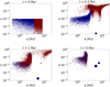 |
Fig. 2 Snapshots of the evolution of planetesimal implantation from a simulation from set 234 starting with 30k planetesimals as the gas giants grow. Terrestrial group material is colour-coded in navy and Jovian group material in burgundy. After 0.3 million years the growing Jupiter is scattering planetesimals away, some of which are circularised by gas drag into the inner Solar System. After 1 Myr the inner Solar System appears to be mostly mixed, and by 5 Myr some embryos can be seen. |
3.1 General evolution and planetesimal implantation
Snapshots of a single simulation from the first simulation set is displayed in Fig. 2; the simulation began with approximately 30k planetesimals plus the seed embryos for the gas giants. The snapshots show the semi-major axis and eccentricity of planetesimals (navy and burgundy dots), and the growing gas giants (large blue dots). The colour-coding of the planetesimals distinguishes terrestrial group (navy) and Jovian group (burgundy) material; in this simulation the assumed initial transition between both reservoirs is at 4 au. As Jupiter grows it begins to scatter the planetesimals in its vicinity, keeping their aphelion or perihelion pegged to the planet, which creates the ‘wings’ seen in the top right and bottom left panels. In the top right panel, after 0.3 million years of evolution, there are burgundy dots with semi-major axis a ~ 2 au and e > 0.3. These bodies have been dynamically decoupled from Jupiter due to gas drag and they will be implanted into the asteroid belt or the terrestrial planet region. After 1 Myr of evolution (bottom left panel) the inner Solar System has become a mixture of navy and burgundy, with small planetary embryos beginning to form near 0.5 au. After 5 Myr (bottom right panel) the asteroid belt beyond 2.5 au has been mostly emptied out, the planetesimals with a > 5 au that were being scattered by the gas giants have also gone, the remaining population of planetesimals in the inner Solar System has a mixed composition, and planetary embryos are clearly visible in the region between 0.5 au and 1 au. The prediction from this simulation is that the material in the inner Solar System has a mixed composition, with the fraction of Jovian material per distant unit expected to increase with increasing distance to the Sun.
A more detailed evolution of the same simulation is given in Fig. 3, which are five two-panel plots at different times. The left column shows the semi-major axis versus mass, the right column the semi-major axis versus eccentricity. The symbol size is proportional to a body’s radius. Red dots are for bodies with a mass <10−3 M⊕, black for masses >0.01 M⊕, and blue for bodies whose masses fall in between these values. The vertical lines denote the approximate transitions of the feeding zones of the terrestrial planets suggested in Woo et al. (2021). In the second row, after 0.25 million years, there are planetesimals with very high eccentricities, e > 0.3, and with semi-major axes a > 2 au. These are the Jovian group planetesimals that are being scattered inwards by the growing Jupiter. In the next panel, after 0.4 million years, the outer part of the asteroid belt with a > 3 au has rising eccentricities, and the outer region is mostly empty after 1 million years of evolution in the fourth row. In the last row, after 5 million years of evolution, the region beyond 2.5 au is empty. The reason for this emptying out is explained in Woo et al. (2021): it is caused by the sweeping of the v5 secular resonance across the asteroid belt as the gas disc’s mass decreases and the precession rate of the asteroids decreases. Those asteroids for which  , where ɡ5 is the secular eigenfrequency corresponding to Jupiter’s perihelion precession, encounter the secular resonance and have their eccentricities pumped to high values (Ward 1981), so that their perihelia decrease and the higher gas surface density closer to the Sun circularises their orbits in the terrestrial planet region. By the end of the simulation several Mars-mass objects have formed in the Venus region, with many Ceres to lunar-mass objects remaining.
3.2 Embryo growth timescales
The average time it takes to grow to a 0.01 M⊕ embryo depends on the initial conditions. For the 232 case, in which bodies grow the fastest, the growth time is  Myr (2σ), which is comparable to what was reported in Woo et al. (2021) (in particular their Fig. 8). For the 334 case I find the same time. For the 315 case, in which growth is one of the slowest, the time taken is about
  Myr, with a similar value for the 234 case,
  Myr, and 335 (
 Myr). For the other sets of simulations the time taken to grow to a lunar mass falls in between.
The growth timescale of Mars has been deduced from Hf-W chronology to be about 5 Myr (Dauphas & Pourmand 2011). In that work, the authors use the parametric growth expression of Mars as M(t) = MMars tanh3(t/τ), with τ = 1.8 ± 0.9 Myr. Following Woo et al. (2021), in Fig. 5 I have plotted this growth curve and three cases of planetary growth from sets 222g4 and 334, wherein a planetesimal collides with multiple bodies to become a Mars-sized embryo, and which grew in the vicinity of 1.5 au from the Sun. As is clear, the growth rate of these embryos is consistent with the range of timescales advocated by Dauphas & Pourmand (2011), but they are generally on the slow end. After 5 million years the average number of embryos per simulation more massive than 0.01 M⊕ is 20–30.
3.3 Embryo composition
The final mass-semi-major axis distribution of the embryos with mass m > 0.01 M⊕ of the different sets of simulations is depicted in Fig. 4. The colour-coding indicates the mass fraction, ƒT, of each body that comes from the terrestrial group; the mass fraction of Jovian material is necessarily ƒ = 1 − ƒT. Some small embryos close to the lunar mass can have high (>25%) fractions of Jovian material incorporated through collision(s) with Jovian group planetesimals. What is immediately clear is that the implantation model creates a compositional gradient similar to what was found by Raymond & Izidoro (2017a): less Jovian material reached the inner regions of the Solar System than father out. The Mercury region closer than 0.5 au has up to 5% Jovian material while near the present orbit of Mars this fraction is typically 20%.
An additional trend is also clear. The top three panels and the bottom left panel all begin with 2 M⊕ of terrestrial group material spread over 1.5 au, 2.5 au, 3.5 au and 1.5 au, respectively. The 3 M⊕ of Jovian material is spread across 6.5 au, 5.5 au, 4.5 au and 4.5 au, respectively. The mostly constant mass of terrestrial group material between these simulations necessarily implies that the surface density of solids decreases as the width of its annulus decreases, which automatically explains why the top left (232) and bottom left (222g4) panels have the most massive embryos and the top right-panel has the least massive embryos (the reason for the difference between the middle left (334) and middle right (335) panels is not clear, but could be due to the different initial number of planetesimals). Clearly the implantation of Jovian group material cannot compensate for the decreasing surface density of the terrestrial group material in speeding up embryo growth.
A different visualisation of the distribution of Jovian group material is shown in Fig. 6 as a function of final semi-major axis of the planets. At the end of the simulations all embryos were binned in semi-major axis bins of 0.1 au and the mass-weighted average fraction plus 1σ uncertainties of Jovian group material was computed. A non-mass-weighted version of this figure is shown in Appendix A. The mass fraction of Jovian group material absorbed by the embryos generally increases with heliocentric distance, with a typical mean value of ƒJ ~ 15% (see Appendix A). However, due to the mass-semi-major axis distribution of the embryos themselves, the mass-weighted fraction of Jovian material is either flat for a > 0.7 au, or bimodal, with peaks at 0.9 au and 2 au. Some embryos beyond 2 au have ƒJ ≳ 35%: these bodies are stranded embryos which consist almost entirely of Jovian group material. Subsequent dynamical evolution will reveal where these bodies end up. The results displayed in Fig. 6 make predictions for the composition of the terrestrial planets once these simulations are continued. Even though generally the feeding zones of the terrestrial planets greatly overlap (e.g. Chambers 2001; Kaib & Cowan 2015; Mah & Brasser 2021), the outcomes shown here predict that Earth analogues are going to have a greater proportion of Jovian group material than Mars analogues if the feeding zones do not overlap too much (Mah & Brasser 2021) This outcome seems to be supported by recent cosmochemical studies (e.g Dauphas et al. 2024; Kleine et al. 2023). Future work will reveal whether this prediction can be reproduced dynamically.
The same final outcomes of some of the simulations is shown in Fig. 7, this time depicting the eccentricities versus semi-major axis of planets, and also of the planetesimals. For this figure, every body with a mass m > 0.01 M⊕ is considered an embryo, and everything else is considered a planetesimal. The colour-coding is the same as in the previous figure and the size of the symbols is proportional to a body’s mass. Red dots indicate planetesimals from the assumed Jovian region while black planetesimals originated from the assumed terrestrial region. It is clear that the planetesimals are thoroughly mixed, apart from in the top panel where the planetesimals with a > 2 au are predominantly red. This has implications for the composition of late accretion impactors on the terrestrial planets after the Moon-forming event.
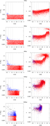 |
Fig. 3 Snaphots of the evolution of a simulation from set 232. Implantation is ongoing at 250 kyr, while after 400 kyr the v5 secular resonance begins to sweep across the asteroid belt. Red dots are bodies with mass <10−3 M⊕, blue dots are for 10−3 < m < 10−2 M⊕, and black dor for more massive bodies. |
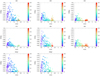 |
Fig. 4 Embryo composition after 5 Myr. The panels show the final semi-major axis versus mass of the embryos for all seven sets of simulations. The colour-coding depicts the fraction of embryo mass that comes from the Jovian group. I note that there is a composition gradient, with the embryos close to 0.5 au having 5% of their mass from the Jovian region while this is closer to 20% for embryos at 1.5 au. |
 |
Fig. 5 Growth tracks of embryos from the 222g4 and 334 sets that grow to Mars’ mass. All three of these remained near 1.5 au in the simulations. |
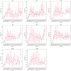 |
Fig. 6 Plots of the mass-weighted average and standard deviation uncertainties of the fraction of Jovian material in planetary embryos after 5 Myr per unit semi-major axis for the different sets of simulations. The quantity plotted is memb ƒJ in units of 10−2 M⊕. |
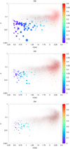 |
Fig. 7 Snapshots of the final semi-major axis and eccentricity distribution of embryos and planetesimals for the simulation sets 232, 233 and 234, showing the decreasing efficiency of embryo formation. Apart from the top panel, the planetesimal population closer than 2.5 au is completely mixed (black for terrestrial group material, red for Jovian group material). Almost no planetesimals reside on orbits with a > 2.5 au. The colour bar shows the fraction of Jovian group material incorporated in the embryos. |
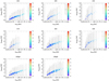 |
Fig. 8 Approximate feeding width of the embryos, depicting the final semi-major axis (x) vs the mass-weighted mean semi-major axis of the accreted material (y). The vertical error bars show the standard deviation and/or range of the feeding zones. There is a clear correlation between the final and mass-weighted semi-major axis, showing that accretion is still mostly from the inner Solar System, but with a large random component due to stochastic accretion of some outer Solar System material. The colour-coding indicates the initial semi-major axis of the embryo. For some small embryos this value is large because they came from beyond the composition changeover distance and went through a few mergers with material from the outer region. The accretion zones of all embryos overlap. |
3.4 Feeding zones and implantation efficiency
For each embryo I tracked their accretion histories and computed their feeding zones. This method is a proxy for the region in the protoplanetary disc from which the embryos sample most of their mass. The feeding zone of an embryo is quantified by the mean aweight and width σweight of the initial semi-major axes of the solids accreted by it throughout its growth history, weighted by their masses (Kaib & Cowan 2015). These quantities are expressed mathematically as (Woo et al. 2018)
 (7)
(7)
and
 (8)
(8)
where mi and ai are the mass and semi-major axis of the ith body accreted by the embryo, and N is the total number of bodies accreted. Together, (aweight ± σweight) define the feeding zone, although in practice this region is not symmetric.
In Fig. 8, I plot the final semi-major axis of the embryos versus their mass-weight semi-major axis computed above after 5 Myr of evolution. The colour-coding indicates their original semi-major axis, symbol sizes are proportional to the mass of a body, and the error bars are the σweight values. The colour-coding indicates that, apart from the very middle panel, most embryos began as planetesimals with semi-major axis ainit < 2 au because that is where most of the mass in planetesimals is initially concentrated. Each panel shows a linear correlation between afinal and aweight. This finding is in contrast to the results by Woo et al. (2021), who found no such correlation. However, Woo et al. (2021) explain the lack of such a correlation due to the migration of embryos. Once they removed the effects of migration, or when the gas giants are assumed to reside on circular orbits, the correlation is obtained. In the top row the slope of the linear correlation increases: in the top left (232) panel the value of aweight ~ 1.8 au when afinal ~ 1.25 au, while this increases to aweight ~ 3 au in the top right (234) panel. This agrees with the result of Fig. 4 where the top right (234) panel appears to have more Jovian material implanted than the top left (232) panel. Thus, even though the embryos become smaller due to the decreasing surface density of terrestrial material, they absorb a greater fraction of Jovian material than their more massive counterparts in the simulations of the top left (232) panel, so that their mass-weighted semi-major axes are skewed higher.
To drive this point home I repeated the same calculation but I ignored all mass incorporated from the Jovian group. The result is displayed in Fig. 9. Once again a correlation is visible, but the slope is much lower, aweight never exceeds 2 au and the feeding zones are much reduced. The width of the feeding zones are comparable to those of the Circular Jupiter and Saturn (CJS) and no gas disc cases of Woo et al. (2021) (i.e. σweight ~ 0.25–0.5 au). The striking difference between the width of the feeding zones with and without including the Jovian group material cautions against using a single parameter to compute the feeding zones, and that the incorporation Jovian group material plays an important role in the final isotopic and elemental composition, in particular for volatile accretion and retention.
I can quantify the amount of mass in embryos, and in planetesimals, that consist of terrestrial and Jovian group material, respectively. I further list the total mass in embryos that arrives from the Jovian reservoir, and the average embryo mass in Table 2. The average mass fraction of Jovian material incorporated in the embryos ranges from 8.9% to 30%, while the mass fraction of Jovian group material ending up in the inner Solar System ranges from 8% to 45%, decreasing as the boundary us moved farther out, and further depending on the outer disc mass.
My implantation efficiency for material coming from beyond 5 au is about 20%, which is comparable but slightly higher than the value found by Raymond & Izidoro (2017a).
It has been suggested that the group of carbonaceous chondrite meteorites span a range of formation distances in the outer Solar System (e.g. Van Kooten et al. 2016), with the CO, CM, and CV group forming closer to the Sun than the CB, CH, and CR (Marrocchi et al. 2018, 2022), and the CI originating the farthest away (Alexander et al. 2013). Although highly uncertain, the CO-CM-CV group could have originated near Jupiter (Marrocchi et al. 2018) and the CI farther out (Krot et al. 2015). This could suggest that the CB-CH-CR group formed near Saturn, and thus it is interesting to trace how much material from Saturn’s region enters the inner Solar System. The approximate dynamical range of the giant planets is 3.5 Hill radii, so that Jupiter’s dynamical range is 4.2 au to 7.0 au, and Saturn’s is 6.3 au to 8.7 au. I thus consider material with original semi-major axis a > 7 au to come from the Saturn region. I then compute the fraction of Jovian group material that ends up into the inner Solar System that originates from Saturn’s region. Figure 10 shows the cumulative distribution of the initial semi-major axis of Jovian group material that was implanted into the inner Solar System for the 232 and 235 sets of simulations; these two span the range of possibilities. From the figure I conclude that from 10% to 30% of Jovian group material that ends up in the inner Solar System originated in the Saturn region, depending on where the boundary between the two groups wa. In other words, of the Jovian group material that made it into the inner Solar System, on average ~ 20% came from the Saturn region. From Table 2 I roughly compute the total amount of mass in planetesimals that originated from the Saturn region was 0.1–0.2 M⊕.
The final thing I report on is that typically the fraction of planetesimals implanted beyond Saturn is 10−4. This is much lower than that of Raymond & Izidoro (2017a). However, their implanted planetesimals beyond Saturn were all 100 km in diameter, or smaller. None of my planetesimals are smaller than 600 km in diameter, and indeed Raymond & Izidoro (2017a) report almost no planetesimals being parked on stable orbits beyond Saturn when their planetesimal diameter is 1000 km. Thus I consider my results to be in agreement with theirs.
However, these outcomes should be interpreted with caution because they will depend on the formation time and formation locations of Uranus and Neptune, which are mostly unknown at present (e.g. Raorane et al. 2024).
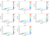 |
Fig. 9 Same as Fig. 8, but ignoring the mass accreted from Jovian group material. It is clear that the feeding zones are much narrower and the correlating slope is much shallower. This shows that incorporation of Jovian group material plays an important role in final composition. |
The final parameters of the simulations in the inner Solar System.
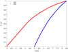 |
Fig. 10 Cumulative distribution of the initial semi-major axis of Jovian group material that ends up in the inner Solar System, for the 232 and 235 sets of simulations. Between 10% to 25% of implanted material could be from the Saturn region, depending on where the composition changeover occurred. |
4 Discussion
The study performed here is a direct continuation of the studies initiated by Raymond & Izidoro (2017a), Woo et al. (2021) and Lau et al. (2024); Raorane et al. (2024). This work is inspired by cosmochemical trends and is an attempt to trace the growth of the terrestrial planets in the presence of the growing gas giants. I go beyond the results of Raymond & Izidoro (2017a) by following the planetesimals scattered inwards by Jupiter and Saturn growing into planetary embryos and, ultimately, into the terrestrial planets in a forthcoming publication. Since this is a first attempt, specific choices were made, which I have outlined above. As always, there is room for improvement if given more time and resources.
First, the growth rate of Jupiter adopted here was very fast, though comparable to what was adopted by Raymond & Izidoro (2017a). However, the pebble accretion simulations of Lau et al. (2024); Raorane et al. (2024) showed that it takes about 1 Myr to form Jupiter’s core, and 3 Myr for Saturn’s. One may debate the validity of these results, but Raorane et al. (2024) showed that the giant planets likely formed sequentially, otherwise Saturn would not have stopped growing at 95 M⊕. It is likely that the cosmochemical dichtomy existed by the time the Solar System was 1–2 Myr old (Kruijer et al. 2017), and irrespective of the mechanism that created it, it is difficult to argue that Jupiter formed earlier than this. As such, a repetition of this study with a slower growth of Jupiter is warranted, and is ongoing.
Second, I have kept the mass of planetesimals in the outer disc mostly at 3 M⊕ and that of the inner disc mostly at 2 M⊕. The choice for the inner disc mass was motivated by the total mass in the terrestrial planets, because I worked under the assumption that the total mass in the inner disc would be mostly preserved. However, spreading this mass over nearly 5 au resulted in a very slow embryo growth, inconsistent with the growth timescale of Mars. Only when the inner disc is truncated at 2 au, and perhaps at 3 au, do I produce Mars-sized embryos within 5 Myr. This may point to a very low surface density having existed in the region of the main asteroid belt at the time that the gas giants formed, but further studies need to rule this in or out.
Third, the high implantation efficiency implies that the fraction of embryo mass with Jovian group material composition is generally more than 10%, seemingly inconsistent with cosmochemical Monte Carlo mixing models (Fitoussi et al. 2016; Dauphas 2017; Dauphas et al. 2024). This problem could be remedied by lowering the mass of the outer disc to 2 M⊕ or even 1 M⊕. Simulations with a 1 M⊕ outer disc indeed predict a lower fraction of Jovian material incorporated, but could pose other problems for giant planet formation.
Fourth, a more contentious issue is the role of the v5 resonance. Woo et al. (2021) discussed at length that the eccentric Jupiter and Saturn (EJS) scenario, in which the resonance operated, was a problem because it and planetary migration caused the planets to all have the same feeding zones. In this study the feeding zones show a clear trend that aweight increases with the final semi-major axis – with and without accounting for the outer disc planetesimals. Thus, it appears that the feeding zone problem that Woo et al. (2021) ran into was more the result of migration rather than the sweeping resonance. Still, a validation of this result with circular Jupiter and Saturn would be warranted.
Fifth, I did not include planet migration for reasons stated earlier: it would cause too much mass to enter the Mercury region of the Solar System, and because of needing to frequently adjust the mGiant parameter while the simulations were running. However, a tentative case could be made that migration is not a huge problem if the terrestrial planets formed from a ring (Izidoro et al. 2022; Woo et al. 2023), or if there was a pressure maximum in the disc near Venus that caused outward migration in the Mercury region (Clement et al. 2021b). A more detailed study with a disc that has a pressure maximum near Venus and one near Jupiter is reserved for future work.
5 Conclusions
I have run numerical N-body simulations of TPF when the gas giants were growing. My main conclusions with the limitations of my study are the following:
Typically 25% of material that is considered isotopically to be of Jovian group composition is implanted in the inner Solar System, depending on where the boundary between the two groups of material is located. Under the assumption that there was initially 3 M⊕ of this material, the implanted mass ranges from 0.66 to 1.8 M⊕;
The implantation efficiency is comparable to that found by Raymond & Izidoro (2017a);
Between 3% and 15% of Jovian group material is incorporated into planetary embryos by 5 Myr. This appears higher than what is suggested from cosmochemical experiments, but can be remedied by lowering the mass of the outer disc;
Embryos have a compositional gradient, with Jovian group material increasing with increasing distance;
Between 0.1 to 0.2 M⊕ implanted in the inner Solar System could have come from the Saturn region. This material could be the source population of the CB, CH and CR carbonaceous chondrites;
Only inner discs truncated at 2 au and possibly at 3 au produce Mars-mass embryos within 5 Myr. This suggests that the current region of the asteroid belt could have had a low initial mass when the Solar System formed;
Remaining planetesimals have a completely mixed composition, which eventually has implications for late accretion.
Future simulations exposing the remaining planetesimals and embryos to late giant planet migration (Tsiganis et al. 2005) and dynamical evolution will reveal whether this scenario is consistent with the isotopic composition of the terrestrial planets.
Acknowledgements
I am thankful to Jason Woo for valuable feedback, Mina Y. Ghodsi for helping with Python plotting, and to John Chambers for acting as a reviewer. I gratefully acknowledge the EuroHPC Joint Undertaking for awarding me access to Vega at IZUM, Slovenia, project EHPC-REG-2022R03-047, and MeluXina at LuxProvide, Luxembourg, project EHPC-REG-2023R03-050. I also acknowledge PRACE for awarding access to the Fenix Infrastructure resources at JUSUF-HPC, Germany, which are partially funded from the European Union’s Horizon 2020 research and innovation programme through the ICEI project under the grant agreement No. 800858. Finally, I acknowledge KIFÜ for awarding me access to the Komondor HPC facility based in Hungary. This study is supported by the Research Council of Norway through its Centres of Excellence funding scheme, project No. 332523 PHAB. GENGA can be obtained from https://bitbucket.org/sigrimm/genga/.
Appendix A Jovian material as a function of heliocentric distance
I show the fraction of Jovian material implanted into the embryos as a function of heliocentric distance, but without mass-weighting. One counter-intuitive result of this figure is that the fraction of Jovian group material in the top left (232) panel is lower than in the top right (234). The reason for this difference is that in the 232 simulations this material is spread over a much wider annulus than in the 234 ones, so that in the the latter simulations less of this material encounters Jupiter and therefore less of it is scattered into the inner Solar System.
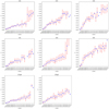 |
Fig. A.1 Plots of the average and standard deviation uncertainties of the fraction of Jovian material in planetary embryos after 5 Myr per unit semi-major axis for the different sets of simulations. |
References
- Alexander, C. M. O. D., Howard, K. T., Bowden, R., & Fogel, M. L. 2013, Geochim. Cosmochim. Acta, 123, 244 [NASA ADS] [CrossRef] [Google Scholar]
- Bédorf, J., Gaburov, E., & Portegies Zwart, S. 2012a, in Advances in Computational Astrophysics: Methods, Tools, and Outcome, eds. R. Capuzzo-Dolcetta, M. Limongi, & A. Tornambè, Astronomical Society of the Pacific Conference Series, 453, 325 [Google Scholar]
- Bédorf, J., Gaburov, E., & Zwart, S. P. 2012b, J. Computat. Phys., 231, 2825 [Google Scholar]
- Brasser, R., & Mojzsis, S. J. 2020, Nat. Astron., 4, 492 [NASA ADS] [CrossRef] [Google Scholar]
- Brasser, R., Werner, S. C., & Mojzsis, S. J. 2020, Icarus, 338, 113514 [NASA ADS] [CrossRef] [Google Scholar]
- Chambers, J. E. 2001, Icarus, 152, 205 [Google Scholar]
- Chambers, J. 2023, ApJ, 944, 127 [NASA ADS] [CrossRef] [Google Scholar]
- Clement, M. S., & Chambers, J. E. 2021, AJ, 162, 3 [NASA ADS] [CrossRef] [Google Scholar]
- Clement, M. S., Kaib, N. A., Raymond, S. N., & Walsh, K. J. 2018, Icarus, 311, 340 [Google Scholar]
- Clement, M. S., Kaib, N. A., Raymond, S. N., Chambers, J. E., & Walsh, K. J. 2019, Icarus, 321, 778 [NASA ADS] [CrossRef] [Google Scholar]
- Clement, M. S., Chambers, J. E., & Jackson, A. P. 2021a, AJ, 161, 240 [NASA ADS] [CrossRef] [Google Scholar]
- Clement, M. S., Raymond, S. N., & Chambers, J. E. 2021b, ApJ, 923, L16 [NASA ADS] [CrossRef] [Google Scholar]
- Dauphas, N. 2017, Nature, 541, 521 [NASA ADS] [CrossRef] [Google Scholar]
- Dauphas, N., & Pourmand, A. 2011, Nature, 473, 489 [NASA ADS] [CrossRef] [Google Scholar]
- Dauphas, N., Hopp, T., & Nesvorný, D. 2024, Icarus, 408, 115805 [NASA ADS] [CrossRef] [Google Scholar]
- Deienno, R., Izidoro, A., Morbidelli, A., Nesvorný, D., & Bottke, W. F. 2022, ApJ, 936, L24 [NASA ADS] [CrossRef] [Google Scholar]
- Deienno, R., Nesvorný, D., Clement, M. S., et al. 2024, PSJ, 5, 110 [NASA ADS] [Google Scholar]
- DeMeo, F. E., & Carry, B. 2014, Nature, 505, 629 [NASA ADS] [CrossRef] [Google Scholar]
- Duncan, M. J., Levison, H. F., & Lee, M. H. 1998, AJ, 116, 2067 [Google Scholar]
- Fitoussi, C., Bourdon, B., & Wang, X. 2016, Earth Planet. Sci. Lett., 434, 151 [CrossRef] [Google Scholar]
- Füri, E., & Marty, B. 2015, Nat. Geosci., 8, 515 [CrossRef] [Google Scholar]
- Gaburov, E., Bédorf, J., & Zwart, S. P. 2010, Procedia Comput. Sci., 1, 1119 [CrossRef] [Google Scholar]
- Grimm, S. L., & Stadel, J. G. 2014, ApJ, 796, 23 [NASA ADS] [CrossRef] [Google Scholar]
- Grimm, S. L., Stadel, J. G., Brasser, R., Meier, M. M. M., & Mordasini, C. 2022, ApJ, 932, 124 [NASA ADS] [CrossRef] [Google Scholar]
- Hansen, B. M. S. 2009, ApJ, 703, 1131 [NASA ADS] [CrossRef] [Google Scholar]
- Hayashi, C. 1981, Progr. Theoret. Phys. Suppl., 70, 35 [CrossRef] [Google Scholar]
- Ida, S., Guillot, T., & Morbidelli, A. 2016, A&A, 591, A72 [NASA ADS] [CrossRef] [EDP Sciences] [Google Scholar]
- Ida, S., Tanaka, H., Johansen, A., Kanagawa, K. D., & Tanigawa, T. 2018, ApJ, 864, 77 [NASA ADS] [CrossRef] [Google Scholar]
- Ikoma, M., Nakazawa, K., & Emori, H. 2000, ApJ, 537, 1013 [NASA ADS] [CrossRef] [Google Scholar]
- Ito, T., Makino, J., Ebisuzaki, T., & Sugimoto, D. 1990, Comput. Phys. Commun., 60, 187 [NASA ADS] [CrossRef] [Google Scholar]
- Izidoro, A., Haghighipour, N., Winter, O. C., & Tsuchida, M. 2014, ApJ, 782, 31 [NASA ADS] [CrossRef] [Google Scholar]
- Izidoro, A., Raymond, S. N., Morbidelli, A., & Winter, O. C. 2015, MNRAS, 453, 3619 [Google Scholar]
- Izidoro, A., Dasgupta, R., Raymond, S. N., et al. 2022, Nat. Astron., 6, 357 [NASA ADS] [CrossRef] [Google Scholar]
- Jacobson, S. A., Morbidelli, A., Raymond, S. N., et al. 2014, Nature, 508, 84 [CrossRef] [Google Scholar]
- Kaib, N. A., & Cowan, N. B. 2015, Icarus, 252, 161 [NASA ADS] [CrossRef] [Google Scholar]
- Kanagawa, K. D., Tanaka, H., & Szuszkiewicz, E. 2018, ApJ, 861, 140 [Google Scholar]
- Kleine, T., Touboul, M., Bourdon, B., et al. 2009, Geochim. Cosmochim. Acta, 73, 5150 [Google Scholar]
- Kleine, T., Steller, T., Burkhardt, C., & Nimmo, F. 2023, Icarus, 397, 115519 [NASA ADS] [CrossRef] [Google Scholar]
- Kokubo, E., & Ida, S. 1995, Icarus, 114, 247 [NASA ADS] [CrossRef] [Google Scholar]
- Kokubo, E., & Ida, S. 1996, Icarus, 123, 180 [Google Scholar]
- Kokubo, E., & Ida, S. 1998, Icarus, 131, 171 [Google Scholar]
- Krot, A. N., Nagashima, K., Alexander, C. M. O., et al. 2015, in Asteroids IV, eds. P. Michel, F. E. DeMeo, & W. F. Bottke, 635 [Google Scholar]
- Kruijer, T., Touboul, M., Fischer-Gödde, M., et al. 2014, Science, 344, 1150 [NASA ADS] [CrossRef] [Google Scholar]
- Kruijer, T. S., Burkhardt, C., Budde, G., & Kleine, T. 2017, PNAS, 114, 6712 [NASA ADS] [CrossRef] [Google Scholar]
- Kruijer, T. S., Kleine, T., & Borg, L. E. 2020, Nat. Astron., 4, 32 [Google Scholar]
- Kruijer, T. S., Archer, G. J., & Kleine, T. 2021, Nat. Geosci., 14, 714 [NASA ADS] [CrossRef] [Google Scholar]
- Lambrechts, M., & Johansen, A. 2012, A&A, 544, A32 [NASA ADS] [CrossRef] [EDP Sciences] [Google Scholar]
- Lammer, H., Brasser, R., Johansen, A., Scherf, M., & Leitzinger, M. 2021, Space Sci. Rev., 217, 7 [NASA ADS] [CrossRef] [Google Scholar]
- Laskar, J. 1997, A&A, 317, L75 [NASA ADS] [Google Scholar]
- Lau, T. C. H., Lee, M. H., Brasser, R., & Matsumura, S. 2024, A&A, 683, A204 [NASA ADS] [CrossRef] [EDP Sciences] [Google Scholar]
- Levison, H. F., Duncan, M. J., & Thommes, E. 2012, AJ, 144, 119 [NASA ADS] [CrossRef] [Google Scholar]
- Lissauer, J. J. 1987, Icarus, 69, 249 [NASA ADS] [CrossRef] [Google Scholar]
- Mah, J., & Brasser, R. 2021, Icarus, 354, 114052 [NASA ADS] [CrossRef] [Google Scholar]
- Mah, J., Brasser, R., Bouvier, A., & Mojzsis, S. J. 2022, MNRAS, 511, 158 [CrossRef] [Google Scholar]
- Marrocchi, Y., Bekaert, D. V., & Piani, L. 2018, Earth Planet. Sci. Lett., 482, 23 [Google Scholar]
- Marrocchi, Y., Piralla, M., Regnault, M., et al. 2022, Earth Planet. Sci. Lett., 593, 117683 [CrossRef] [Google Scholar]
- Marty, B., Chaussidon, M., Wiens, R. C., Jurewicz, A. J. G., & Burnett, D. S. 2011, Science, 332, 1533 [NASA ADS] [CrossRef] [Google Scholar]
- Matsumura, S., Brasser, R., & Ida, S. 2021, A&A, 650, A116 [NASA ADS] [CrossRef] [EDP Sciences] [Google Scholar]
- Mezger, K., Schönbächler, M., & Bouvier, A. 2020, Space Sci. Rev., 216, 27 [NASA ADS] [CrossRef] [Google Scholar]
- Morbidelli, A., Lunine, J. I., O’Brien, D. P., Raymond, S. N., & Walsh, K. J. 2012, Annu. Rev. Earth Planet. Sci., 40, 251 [CrossRef] [Google Scholar]
- Morbidelli, A., Kleine, T., & Nimmo, F. 2025, Earth Planet. Sci. Lett., 650, 119120 [CrossRef] [Google Scholar]
- Morishima, R., Stadel, J., & Moore, B. 2010, Icarus, 207, 517 [NASA ADS] [CrossRef] [Google Scholar]
- Nesvorný, D., Dauphas, N., Vokrouhlický, D., Deienno, R., & Hopp, T. 2024, Earth Planet. Sci. Lett., 626, 118521 [CrossRef] [Google Scholar]
- O’Brien, D. P., Morbidelli, A., & Levison, H. F. 2006, Icarus, 184, 39 [CrossRef] [Google Scholar]
- Ormel, C. W., & Klahr, H. H. 2010, A&A, 520, A43 [NASA ADS] [CrossRef] [EDP Sciences] [Google Scholar]
- Piani, L., Marrocchi, Y., Rigaudier, T., et al. 2020, Science, 369, 1110 [NASA ADS] [CrossRef] [Google Scholar]
- Raorane, A., Brasser, R., Matsumura, S., et al. 2024, Icarus, 421, 116231 [NASA ADS] [CrossRef] [Google Scholar]
- Raymond, S. N., & Izidoro, A. 2017a, Icarus, 297, 134 [CrossRef] [Google Scholar]
- Raymond, S. N., & Izidoro, A. 2017b, Sci. Adv., 3, e1701138 [NASA ADS] [CrossRef] [Google Scholar]
- Raymond, S. N., Quinn, T., & Lunine, J. I. 2006, Icarus, 183, 265 [Google Scholar]
- Raymond, S. N., O’Brien, D. P., Morbidelli, A., & Kaib, N. A. 2009, Icarus, 203, 644 [NASA ADS] [CrossRef] [Google Scholar]
- Rider-Stokes, B. G., Stephant, A., Anand, M., et al. 2024, Earth Planet. Sci. Lett., 642, 118860 [CrossRef] [Google Scholar]
- Rudge, J. F., Kleine, T., & Bourdon, B. 2010, Nat. Geosci., 3, 439 [NASA ADS] [CrossRef] [Google Scholar]
- Sarafian, A. R., Nielsen, S. G., Marschall, H. R., McCubbin, F. M., & Monteleone, B. D. 2014, Science, 346, 623 [NASA ADS] [CrossRef] [Google Scholar]
- Sarafian, A. R., Nielsen, S. G., Marschall, H. R., et al. 2017, Geochim. Cosmochim. Acta, 212, 156 [NASA ADS] [CrossRef] [Google Scholar]
- Schiller, M., Bizzarro, M., & Fernandes, V. A. 2018, Nature, 555, 507 [Google Scholar]
- Schiller, M., Bizzarro, M., & Siebert, J. 2020, Sci. Adv., 6, eaay7604 [NASA ADS] [CrossRef] [Google Scholar]
- Seager, S., Kuchner, M., Hier-Majumder, C. A., & Militzer, B. 2007, ApJ, 669, 1279 [NASA ADS] [CrossRef] [Google Scholar]
- Tang, H., & Dauphas, N. 2014, Earth Planet. Sci. Lett., 390, 264 [CrossRef] [Google Scholar]
- Thiemens, M. M., Sprung, P., Fonseca, R. O., Leitzke, F. P., & Münker, C. 2019, Nat. Geosci., 12, 696 [NASA ADS] [CrossRef] [Google Scholar]
- Thiemens, M. M., Tusch, J., O. C. Fonseca, R., et al. 2021, Nat. Geosci., 14, 716 [NASA ADS] [CrossRef] [Google Scholar]
- Tsiganis, K., Gomes, R., Morbidelli, A., & Levison, H. F. 2005, Nature, 435, 459 [Google Scholar]
- Van Kooten, E. M. M. E., Wielandt, D., Schiller, M., et al. 2016, PNAS, 113, 2011 [NASA ADS] [CrossRef] [Google Scholar]
- Walsh, K. J., & Levison, H. F. 2019, Icarus, 329, 88 [NASA ADS] [CrossRef] [Google Scholar]
- Walsh, K. J., Morbidelli, A., Raymond, S. N., O’Brien, D. P., & Mandell, A. M. 2011, Nature, 475, 206 [Google Scholar]
- Wang, H., Weiss, B. P., Bai, X.-N., et al. 2017, Science, 355, 623 [NASA ADS] [CrossRef] [Google Scholar]
- Ward, W. R. 1981, Icarus, 47, 234 [NASA ADS] [CrossRef] [Google Scholar]
- Warren, P. H. 2011, Earth Planet. Sci. Lett., 311, 93 [Google Scholar]
- Weiss, L. M., & Marcy, G. W. 2014, ApJ, 783, L6 [Google Scholar]
- Weiss, B. P., Bai, X.-N., & Fu, R. R. 2021, Sci. Adv., 7, eaba5967 [NASA ADS] [CrossRef] [Google Scholar]
- Wetherill, G. W., & Stewart, G. R. 1989, Icarus, 77, 330 [Google Scholar]
- Woo, J. M. Y., Brasser, R., Matsumura, S., Mojzsis, S. J., & Ida, S. 2018, A&A, 617, A17 [NASA ADS] [CrossRef] [EDP Sciences] [Google Scholar]
- Woo, J. M. Y., Grimm, S., Brasser, R., & Stadel, J. 2021, Icarus, 359, 114305 [NASA ADS] [CrossRef] [Google Scholar]
- Woo, J. M. Y., Morbidelli, A., Grimm, S. L., Stadel, J., & Brasser, R. 2023, Icarus, 396, 115497 [NASA ADS] [CrossRef] [Google Scholar]
- Yamakawa, A., Yamashita, K., Makishima, A., & Nakamura, E. 2010, ApJ, 720, 150 [NASA ADS] [CrossRef] [Google Scholar]
- Yin, Q., Jacobsen, S. B., Yamashita, K., et al. 2002, Nature, 418, 949 [CrossRef] [Google Scholar]
- Yokoyama, T., Nagashima, K., Nakai, I., et al. 2022, Science, 379, eabn7850 [Google Scholar]
- Yu, G., & Jacobsen, S. B. 2011, PNAS, 108, 17604 [NASA ADS] [CrossRef] [Google Scholar]
All Tables
All Figures
|
Fig. 1 Growth of the masses of Jupiter and Saturn as a function of time adopted in this study. |
| In the text | |
|
Fig. 2 Snapshots of the evolution of planetesimal implantation from a simulation from set 234 starting with 30k planetesimals as the gas giants grow. Terrestrial group material is colour-coded in navy and Jovian group material in burgundy. After 0.3 million years the growing Jupiter is scattering planetesimals away, some of which are circularised by gas drag into the inner Solar System. After 1 Myr the inner Solar System appears to be mostly mixed, and by 5 Myr some embryos can be seen. |
| In the text | |
|
Fig. 3 Snaphots of the evolution of a simulation from set 232. Implantation is ongoing at 250 kyr, while after 400 kyr the v5 secular resonance begins to sweep across the asteroid belt. Red dots are bodies with mass <10−3 M⊕, blue dots are for 10−3 < m < 10−2 M⊕, and black dor for more massive bodies. |
| In the text | |
|
Fig. 4 Embryo composition after 5 Myr. The panels show the final semi-major axis versus mass of the embryos for all seven sets of simulations. The colour-coding depicts the fraction of embryo mass that comes from the Jovian group. I note that there is a composition gradient, with the embryos close to 0.5 au having 5% of their mass from the Jovian region while this is closer to 20% for embryos at 1.5 au. |
| In the text | |
|
Fig. 5 Growth tracks of embryos from the 222g4 and 334 sets that grow to Mars’ mass. All three of these remained near 1.5 au in the simulations. |
| In the text | |
|
Fig. 6 Plots of the mass-weighted average and standard deviation uncertainties of the fraction of Jovian material in planetary embryos after 5 Myr per unit semi-major axis for the different sets of simulations. The quantity plotted is memb ƒJ in units of 10−2 M⊕. |
| In the text | |
|
Fig. 7 Snapshots of the final semi-major axis and eccentricity distribution of embryos and planetesimals for the simulation sets 232, 233 and 234, showing the decreasing efficiency of embryo formation. Apart from the top panel, the planetesimal population closer than 2.5 au is completely mixed (black for terrestrial group material, red for Jovian group material). Almost no planetesimals reside on orbits with a > 2.5 au. The colour bar shows the fraction of Jovian group material incorporated in the embryos. |
| In the text | |
|
Fig. 8 Approximate feeding width of the embryos, depicting the final semi-major axis (x) vs the mass-weighted mean semi-major axis of the accreted material (y). The vertical error bars show the standard deviation and/or range of the feeding zones. There is a clear correlation between the final and mass-weighted semi-major axis, showing that accretion is still mostly from the inner Solar System, but with a large random component due to stochastic accretion of some outer Solar System material. The colour-coding indicates the initial semi-major axis of the embryo. For some small embryos this value is large because they came from beyond the composition changeover distance and went through a few mergers with material from the outer region. The accretion zones of all embryos overlap. |
| In the text | |
|
Fig. 9 Same as Fig. 8, but ignoring the mass accreted from Jovian group material. It is clear that the feeding zones are much narrower and the correlating slope is much shallower. This shows that incorporation of Jovian group material plays an important role in final composition. |
| In the text | |
|
Fig. 10 Cumulative distribution of the initial semi-major axis of Jovian group material that ends up in the inner Solar System, for the 232 and 235 sets of simulations. Between 10% to 25% of implanted material could be from the Saturn region, depending on where the composition changeover occurred. |
| In the text | |
|
Fig. A.1 Plots of the average and standard deviation uncertainties of the fraction of Jovian material in planetary embryos after 5 Myr per unit semi-major axis for the different sets of simulations. |
| In the text | |
Current usage metrics show cumulative count of Article Views (full-text article views including HTML views, PDF and ePub downloads, according to the available data) and Abstracts Views on Vision4Press platform.
Data correspond to usage on the plateform after 2015. The current usage metrics is available 48-96 hours after online publication and is updated daily on week days.
Initial download of the metrics may take a while.