| Issue |
A&A
Volume 694, February 2025
|
|
|---|---|---|
| Article Number | A31 | |
| Number of page(s) | 9 | |
| Section | Extragalactic astronomy | |
| DOI | https://doi.org/10.1051/0004-6361/202452234 | |
| Published online | 30 January 2025 | |
FBQ 0951+2635: Time delay and structure of the main lensing galaxy
1
Instituto de Física de Cantabria (CSIC-UC), Avda. de Los Castros s/n, E-39005 Santander, Spain
2
Departamento de Física Moderna, Universidad de Cantabria, Avda. de Los Castros s/n, E-39005 Santander, Spain
3
O.Ya. Usikov Institute for Radiophysics and Electronics, National Academy of Sciences of Ukraine, 12 Acad. Proscury St., UA-61085 Kharkiv, Ukraine
⋆ Corresponding authors; This email address is being protected from spambots. You need JavaScript enabled to view it.
; This email address is being protected from spambots. You need JavaScript enabled to view it.
Received:
13
September
2024
Accepted:
10
December
2024
Abstract
As there is a long-standing controversy over the time delay between the two images of the gravitationally lensed quasar FBQ 0951+2635, we combined early and new optical light curves to robustly measure a delay of 13.5 ± 1.6 d (1σ interval). The new optical records covering the last 17 yr were also used to trace the long-timescale evolution of the microlensing variability. Additionally, the new time-delay interval and a relatively rich set of further observational constraints allowed us to discuss the mass structure of the main lensing galaxy at a redshift of 0.26. This lens system is of particular interest because the external shear from secondary gravitational deflectors is relatively low, but the external convergence is one of the highest known. When modelling the galaxy as a singular power-law ellipsoid without hypotheses or priors on the power-law index, ellipticity, and position angle, we demonstrated that its mass profile is close to isothermal, and there is a good agreement between the shape of the mass distribution and that of the near-IR light. We also recovered the true mass scale of the galaxy. Finally, a constant mass-to-light ratio model also worked acceptably well.
Key words: gravitational lensing: strong / galaxies: structure / quasars: individual: FBQ 0951+2635
© The Authors 2025
 Open Access article, published by EDP Sciences, under the terms of the Creative Commons Attribution License (https://creativecommons.org/licenses/by/4.0), which permits unrestricted use, distribution, and reproduction in any medium, provided the original work is properly cited.
This article is published in open access under the Subscribe to Open model. This email address is being protected from spambots. You need JavaScript enabled to view it. to support open access publication.
1. Introduction
Strong gravitational lensing at the galaxy scale is a key tool for investigating the structure of non-local early-type galaxies (e.g., Koopmans et al. 2006; Shajib et al. 2024). When the lensed source is a quasar, the mass distribution of the main lensing galaxy can be probed with a suitable number of observational constraints. Although deep photometric observations with the Hubble Space Telescope (HST) or ground-based facilities incorporating adaptive optics provide images of the quasar host galaxy (e.g., Wong et al. 2020), the basic constraints consist of the positions of the quasar images and the light distribution of the main lens. In addition to these basic astro-photometric data, deep spatially resolved spectroscopy of the system is required to estimate unbiased macro-magnification ratios, that is, the flux ratios between quasar images that are not affected by extinction, microlensing, and intrinsic variability effects (e.g., Sluse et al. 2012b; Goicoechea & Shalyapin 2016). Radio fluxes, if available, are expected to be not affected by microlensing (large source) and dust extinction (long wavelength), and radio flux ratios at a single epoch are therefore good proxies of the macro-magnification ratios for a lensed quasar with short delays between images. Sometimes, a smoothly distributed lensing mass fails to reproduce the measured macro-magnification ratios of a lensed quasar, and these flux ratio anomalies may be caused by the galaxy substructures (millilensing; e.g., Metcalf & Madau 2001). Millilensing effects would be different for broad emission lines, radio fluxes, and narrow emission lines because they depend on the source size (e.g., Moustakas & Metcalf 2003).
According to Refsdal’s 60-year old ideas (Refsdal 1964), the time delays between quasar images from photometric monitoring campaigns can also be used to constrain the mass distribution of the main lens when the spectroscopic redshifts of the source and main lens are known and the main cosmological parameters are derived from independent experiments (e.g., Hinshaw et al. 2009; Planck Collaboration VI 2020). Additionally, information about the stellar kinematics of the main lens, or about the secondary deflectors around the main one and along the line of sight, is required to reliably probe the mass distribution of the main lensing galaxy (e.g., Falco et al. 1985; Suyu et al. 2010). This last information is currently only available for a relatively small number of lensed quasars with detailed studies on the stellar kinematics of their main lenses (e.g., Birrer et al. 2020; Shajib et al. 2023), or on the main lens environments and line-of-sight deflectors (e.g., Rusu et al. 2017; Wilson et al. 2017).
FBQ 0951+2635 is a doubly imaged quasar that was discovered by Schechter et al. (1998). This lensed quasar is located at a redshift zs = 1.249 (Momcheva et al. 2015), and the main lens is an early-type galaxy at zl = 0.260 (Eigenbrod et al. 2007). It is a particularly interesting lens system for several reasons. First, even though near-IR HST imaging of FBQ 0951+2635 (Kochanek et al. 2000) led to two formally precise solutions for the relative astrometry of the system and the morphology of the early-type galaxy (Jakobsson et al. 2005; Sluse et al. 2012a), these solutions are not consistent with each other. Thus, we aim to study how the two astro-photometric datasets influence the reconstruction of the lensing mass. Although the near-IR morphology of the galaxy basically consists of a prominent elliptical halo, Rivera et al. (2023) very recently suggested the existence of an additional feature: a faint edge-on disc. In this paper, we do not consider the minor features that require confirmation through new observations. Second, there are spectroscopic observations with large optical telescopes in very good seeing conditions and radio fluxes at 3.6 cm from the Very Large Array (VLA) that can be used to obtain a reliable constraint on the macro-magnification ratio (e.g., Jakobsson et al. 2005; Sluse et al. 2012b). Third, Wilson et al. (2017) quantified the gravitational-lensing effect of galaxy groups at the main lens redshift and along the line of sight.
We also used the time delay between the two quasar images as an important constraint on the mass distribution of the non-local early-type galaxy. However, current values of the time delay of FBQ 0951+2635 are not trustworthy. Optical light curves in the period 1999–2001 were initially analysed by Jakobsson et al. (2005), who obtained a time delay of 16 ± 2 d (the brightest image is leading) using the last 38 data points. Although these last data seem to be weakly affected by extrinsic (microlensing) variability, an iterative fit yielded a time delay of 13 ± 4 d using all (58) data points, that is, having twice the uncertainty and a significantly shorter central value. From the same dataset, Eulaers & Magain (2011) found that different time-delay values in the 10–30 d interval are possible, whereas Rathna Kumar et al. (2015) measured a time delay of 7.8 ± 14.0 d. The obvious conclusion is that additional data are required to reliably measure the time delay of the system.
The paper is organized as follows. In Sect. 2, we analyse optical light curves of FBQ 0951+2635 spanning 25 yr (1999–2024) to determine a reliable time delay between the two quasar images and identify the long-term microlensing signal. Sect. 3 includes the observational constraints for the lens system, as well as the method we used to probe the mass distribution of the main lensing galaxy and the results on its structure. In Sect. 4, we present our main conclusions.
2. Optical light curves and time delay
2.1. Light curves
The first optical monitoring campaigns of FBQ 0951+2635 focused on the R passband. Thus, based on observations with the Nordic Optical Telescope (NOT) at 58 epochs (nights), Jakobsson et al. (2005) and Paraficz et al. (2006) presented R-band light curves of the two quasar images (A and B) from 1999 to 2001. A monitoring programme with the main Maidanak Telescope (MT) in the period 2001–2006 also led to R-band light curves at 37 epochs (Shalyapin et al. 2009).
After the pioneering variability records from NOT and MT observations, we monitored FBQ 0951+2635 as part of the Gravitational LENses and DArk MAtter (GLENDAMA) project (Gil-Merino et al. 2018) with the Liverpool Telescope (LT) in the optical r band from 2009 to 2024. Over the full monitoring period, r-band magnitudes at 142 epochs were obtained (the photometric model and initial LT light curves were presented by Gil-Merino et al. 2018). We then combined the LT magnitudes and those obtained with the Kaj Strand Telescope (KST) during 2008–2017 (Rivera et al. 2023), removed two KST epochs at MJD = 54883 and 57866 with possible outliers, corrected for small magnitude offsets between the Tek2k and OneChip cameras in the KST (image A and B offsets of −0.001 and +0.005 mag for OneChip respect to Tek2k), and shifted the KST magnitudes to the LT system (+16.879 and +16.809 mag for A and B, respectively). We point out that magnitude offsets are estimated in a standard way by comparing concurrent data from two different cameras or telescopes. In addition, photometric errors rely on the intra-night magnitude scatter drawn from the analysis of two or three individual frames each night. Possible outliers were also removed as they might affect the time-delay measurements.
To improve the sampling over the period 2008–2024, we added several r-band magnitudes (LT photometric system) from data release 1 of the Panoramic Survey Telescope and Rapid Response System1 (Pan-STARRS or PS; Flewelling et al. 2020), and data release 2 of the Dark Energy Survey2 (DES; Abbott et al. 2021). The new 17 yr brightness records including magnitudes at 213 epochs are available in Table 1 at the CDS (see Sect. “Data availability”). These LT-KST-PS-DES (GLENDAMA+) light curves are also displayed in Figure 1.
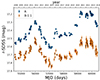 |
Fig. 1. GLENDAMA+ light curves of FBQ 0951+2635. These new variability records mainly consist of photometric data from the LT (circles) and KST (squares), but also incorporate information provided by the PS (inverted triangles) and DES (triangles) databases. See main text for details. |
2.2. Time-delay measurement
The R-band NOT light curves did not permit us to measure a time delay between A and B with a precision of ∼10%. The analysis of Jakobsson et al. (2005) suggested a delay interval of 10–20 d (depending on the technique, the smoothing, and the data points used), and subsequent studies indicated delay intervals of 10–30 d (Eulaers & Magain 2011) and even included negative values, that is, image B leads image A (Rathna Kumar et al. 2015). Hence, additional light curves are required to address time delay measurements to ∼10%, and we considered the NOT dataset along with the GLENDAMA+ data. There is clear evidence for intrinsic variations in the 2008–2024 period because the brightness changes of A and B are significantly greater than the photometric uncertainties, and additionally, A and B show an almost parallel behaviour (see Figure 1).
Because the optical light curves of FBQ 0951+2635 are affected by a long-timescale microlensing episode (e.g., Shalyapin et al. 2009; Rivera et al. 2023), we measured the time delay using cross-correlation techniques that account for extrinsic variability. We developed easy-to-use Python scripts to estimate the time delay of a doubly-imaged quasar with two different methods incorporating polynomial microlensing variability. These scripts are publicly available at GitHub3 and briefly described in Appendix A. The first method we used is the most sophisticated variant of the dispersion technique (D42; Pelt et al. 1996), which relied on a weighting scheme for the squared differences between the B image data and shifted A image data, where the A image data were shifted by a time lag τ and a microlensing polynomial of degree Nml. Our Gaussian weighting scheme is characterised by a parameter β and is outlined in Appendix A. After we set values for Nml and β, the dispersion spectrum D42 was computed as the weighted sum of the squared differences for time lags within a reasonable interval. To build this spectrum, we previously solved the microlensing polynomial coefficients that minimise it for each τ value. The time delay was assumed to be the time lag that minimises the dispersion spectrum.
Considering polynomials of different degrees and several values of the parameter β, we verified that the minimum dispersions decreased when the polynomial degree was progressively increased up to Nml = 5, while a polynomial of degree Nml = 6 did not produce substantial decreases in the minimum dispersions. For Nml = 5 and a broad range of β values (3 < β < 30 d), we found stable minima in the D42 spectra covering the time lag interval [−50, +50] d. Some of these spectra with minima at 13–15 d are shown in the top panel of Figure 2.
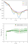 |
Fig. 2. Time-delay estimation from the dispersion technique. The dispersion spectra D42 are based on a Gaussian weighting function whose width is described by the parameter β, as well as a fifth-degree microlensing polynomial (Nml = 5; see main text). Top panel: D42 spectra using the NOT light curves plus the new GLENDAMA+ brightness records and five values of β. These spectra have minima at time lags τ = 13–15 d. Bottom panel: 1σ confidence intervals for the time delay using 1000 synthetic light curves of each image and a large set of β values. A combined measurement from the six delay intervals for β = 4–9 d is highlighted with a light grey rectangle encompassing the individual measurements. |
To quantify the delay uncertainties, we generated 1000 synthetic light curves of each image based on the observed records (e.g., Shalyapin & Goicoechea 2017). More precisely, we made 1000 repetitions of the experiment (synthetic curves for A and B) by adding random quantities to the measured magnitudes. These random quantities were realisations of normal distributions around zero, with standard deviations equal to the measured errors. We did not exactly repeat the original experiment, but rather a worsened experiment with errors greater than those observed, that is, the simulated magnitudes were not derived through a reconstruction of the underlying signal, but from the observed signal. Our simulation scheme is thus conservative regarding the size of error bars (about 20% larger than the measured errors), with the caveat that only uncorrelated noise was added. We obtained distributions of time lags and polynomial coefficients that minimised the D42 spectra from the simulated records. We then searched for minima within the interval [−30, +30] d to speed up the numerical calculations involving thousands of dispersion spectra. However, for certain β values, we checked that the results using this narrower range of time lags are basically identical to those using the interval [−50, +50] d.
For β = 3 d, local minima in D42 play a role, while for β > 10 d, the dispersion minima are shallow and the delay uncertainties are relatively large. For β = 4–9 d, the time-delay values are around 13–14 d with 1σ errors smaller than 2 d (see the bottom panel of Figure 2). We then combined (averaged) these six precise delay measurements to obtain the 1σ confidence interval 13.5 ± 1.6 d (light grey rectangle). The central values of the individual delays were averaged to find the mean value, and the uncertainty was computed as the square root of the sum of the squares of two contributions: the standard error of the mean value, and the average of individual delay errors.
The time delay of FBQ 0951+2635 was also measured from a variant of the χ2 technique. The A image data were shifted by a time lag τ and a fifth-degree microlensing polynomial (Nml = 5), and they were then compared with B image data binned around the time-shifted dates of A. The bins with a semi-size α were constructed through a linear weighting function, and for a given value of α, we used a reduced chi-square (χr2) minimisation to estimate the polynomial coefficients and time lag that caused the shifted light curve of A and the binned brightness record of B to match (see details in Appendix A). We remark that a polynomial with Nml< 5 leads to relatively high minimum χr2 values, and the minimum χr2 values for Nml = 5 are barely modified for Nml = 6. Thus, the choice Nml = 5 is justified for the χr2 method. The PyCS3 software4 (e.g., Tewes et al. 2013; Millon et al. 2020a) includes another variant of the χ2 technique for estimating the time delays between images of gravitationally lensed quasars. However, the intrinsic variability is modelled as a free-knot spline, and we therefore adopted a simpler scheme to avoid fitting a complex intrinsic signal.
For 3 < α< 30 d, the 1000 simulated light curves of each quasar image (see above) allowed us to calculate 1σ confidence intervals for the time delay (see Figure 3). We searched again for minima within the interval [−30, +30] d, but checked the absence of border biases by using a second more extended interval [−50, +50] d for several α values. Excessively low or high values of α (or β for the minimum dispersion method; see above) are not suitable for time-delay estimates. For α≥ 12 d, the χr2 minima are affected by systematics (sudden drops in χr2 at certain time lags) or are shallow. The mentioned systematics cause the anomalous delay-α relation for α = 12–16 d (see the black outlined rectangle in Figure 3). This anomaly consists of a set of formally ultra-precise delays around 14 d that are not consistent with each other. For α = 5–11 d, the delay estimates are consistent with the results from the dispersion technique, and the two most precise measurements (for α = 5 and 11 d) agree very well with the dispersion-based delay of 13.5 ± 1.6 d. We also note that the minima in χr2 for α = 5 and 11 d are derived from ∼140 and ∼190 AB data pairs, respectively, so there is a significant overlap between the records of A and B.
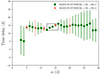 |
Fig. 3. Time-delay estimation from the χr2 technique and 1000 synthetic light curves of each quasar image. To match the light curves of the two images, a fifth-degree microlensing polynomial and binned light curves of B were considered, where bins of the B image have a semi-size α. The error bars represent 1σ confidence intervals for the time delay, and the black outlined rectangle contains five anomalous measurements (see main text). |
2.3. Long-term microlensing
To trace the long-timescale extrinsic (microlensing) signal in the red optical passbands, we built the difference light curve (DLC) from 1999 to 2024 (see Figure 4). This historical DLC relies on the R-band NOT-MT light curves and the GLENDAMA+ records in Figure 1, and it consists of the differences between the image B magnitudes at original epochs and the image A magnitudes shifted by the time delay Δt = 13.5 d, that is, mB(t)−mA(t − Δt). The differences were determined by linear interpolation of the time-shifted record of A. Figure 4 also displays dispersion-based solutions of the fifth-degree microlensing polynomial (thick solid line), which result from 1σ confidence intervals of the polynomial coefficients for 3 < β< 30 d. Although these solutions were obtained using only NOT and GLENDAMA+ data (filled circles), they predict the DLC shape at intermediate epochs reasonably well (open circles; however, as expected, the solutions do not account for the bump around day 53 000 reported by Shalyapin et al. 2009). The DLC has evolved from an initial value close to 1 mag at the end of the last century to 1.4–1.5 mag in the current decade. Hence, some recent DLC values are roughly consistent with the B/A flux ratio from radio observations and emission lines (see Sect. 3.1).
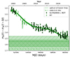 |
Fig. 4. New 25 yr DLC of FBQ 0951+2635 in the red optical passbands from NOT-MT and GLENDAMA+ data. We also show solutions of the fifth-degree microlensing polynomial (thick solid line; see main text for details). For comparison purposes, we include the magnitude differences from VLA data (horizontal dash-dotted line; Jakobsson et al. 2005) and emission lines (horizontal dashed line; see Sect. 3.1). The striped rectangles represent the uncertainties in these two differences. |
3. Observational constraints and structure of the main lensing galaxy
3.1. Observational constraints
We focused on the double quasar FBQ 0951+2635 and present details on its observational constraints that we summarise in Table 2. The spectroscopic redshifts of the source and the main lensing galaxy G are cited in Sect. 1. Jakobsson et al. (2005) and Sluse et al. (2012a) also used near-IR HST imaging (Kochanek et al. 2000) to determine the relative astrometry of the system and the morphology of the early-type galaxy G, whose brightness profile was modelled by a De Vaucouleurs law. However, the two independent analyses of the same data yielded two astro-photometric solutions (APS 1 and APS 2) that differ in image separation, that is, the angular distance between A and B, and the galaxy morphological parameters (see Table 2). Additionally, the discovery paper (Schechter et al. 1998) reported VLA radio fluxes of both quasar images, which led to a radio flux ratio B/A = 0.21 ± 0.03 (mB − mA = 1.69 ± 0.16 mag) at 8.4 GHz (Jakobsson et al. 2005).
Summary of the observational constraints of FBQ 0951+2635.
Using optical spectra of FBQ 0951+2635 from the Keck II Telescope (Schechter et al. 1998), the Very Large Telescope (Eigenbrod et al. 2007), and the William Herschel Telescope (Fian et al. 2021), we also estimated the flux ratio B/A for the cores of the C IV, C III], and Mg II emission lines. The six B/A values range bewteen 0.20 and 0.26, and a basic statistics of these six estimates (mean = 0.24 and standard deviation = 0.02, or equivalently, mB − mA = 1.55 ± 0.09 mag) agrees well with the radio flux ratio (see above) and the macro-magnification ratio M in Table 4 of Sluse et al. (2012b). We then adopted the constraint of Sluse et al. on M. In addition to the spectroscopic test of the macro-magnification ratio, we present a time-delay measurement to ∼10% by combining early optical light curves and those through observations made over the last 17 yr (see Sect. 2.2). In the near future, better photometric data in more densely sampled light curves might lead to a delay error smaller than 1.5 d. However, taking a possible microlensing-induced scatter of ∼1 d into account (e.g., Tie & Kochanek 2018), this perspective may be excessively optimistic.
The time delay between the two images of a double quasar is basically given by the product of the time-delay distance and the Fermat potential variation between the two images (e.g., Treu & Marshall 2016; Suyu et al. 2018). The Fermat potential variation relies upon the lensing mass distribution. In addition, the time-delay distance depends on zs and zl, and it is inversely proportional to H0, with other cosmological parameters playing a lesser role. For consistency with current constraints on secondary deflectors (see below), we adopted a flat ΛCDM cosmology with H0 = 71 km s−1 Mpc−1, ΩM = 0.274, and ΩΛ = 0.726 (Hinshaw et al. 2009; Komatsu et al. 2009). Using these cosmological parameters, Wilson et al. (2017) focused on determining the gravitational lensing effect of galaxy groups for FBQ 0951+2635, that is, the group to which G belongs (environment of G) and additional line-of-sight groups. They did not explore the minor influence of isolated galaxies on the lensing potential, and they estimated the typical values of the external convergence (κext), external shear strength (γext), and position angle of the external shear (θγext) that are shown in Table 2.
3.2. Method for reconstructing the mass distribution of the main deflector
The lensing mass distribution was initially modelled using two standard components: a singular power-law ellipsoid (SPLE) to describe the main lensing galaxy G, and an external shear caused by the additional mass intervening (e.g., Suyu et al. 2013; Shajib et al. 2019). Although an SPLE is often characterised by its logarithmic mass-density slope γ, we used the power-law index αpl (αpl = 3 − γ) to avoid any confusion with the shear and to be consistent with the notation in the model catalogue of the GRAVLENS/LENSMODEL software (Keeton 2001, 2002). Although neither the light nor the dark matter distribution in galaxies follow a power-law radial profile, the combined (total) density profile of G is expected to be close to isothermal (SPLE with αpl∼ 1; e.g., Koopmans et al. 2006; Capellari et al. 2015; Wang et al. 2020; Sheu et al. 2024). It is also noteworthy that the quasi-isothermal combined model leads to similar results as a model that treats light and dark matter individually (e.g., Suyu et al. 2014; Millon et al. 2020b). For comparison purposes, we also considered a constant mass-to-light ratio model of G, that is, a De Vaucouleurs (DV) surface mass density instead of that for a SPLE.
In addition to the power-law index, the parameters of the SPLE model were the 2D position (x0, y0), the mass scale5b, the ellipticity e, and the position angle θe. The external shear is also described by two parameters: the strength γext, and the position angle θγext, whereas it is not necessary to explicitly incorporate the external convergence into the lensing mass model. However, if κext ≠ 0, some model parameters must be appropriately reinterpreted (e.g., Falco et al. 1985; Grogin & Narayan 1996). We mean b ↦ b* = b/(1 − κext)1/(2 − αpl) and  , as well as H0 ↦ H0* = H0/(1 − κext) (e.g., Fadely et al. 2010). For example, for this system with such high external convergence (see Table 2), the use of H0* (instead of H0) plays a critical role when the time delay is considered as a constraint on the mass distribution.
Setting the values of zs, zl,  , θγext, H0*, ΩM, and ΩΛ, and taking 1σ confidence intervals for the positions of A, B and G, the macro-magnification, and the time delay (see Sect. 3.1), the GRAVLENS/LENSMODEL software allowed us to fit the six parameters of the SPLE model (see above). Because we considered two astro-photometric solutions (APS 1 and APS 2), we obtained two different reconstructions of the SPLE mass distribution. We note again that we fit the effective mass scale b* in our model, so that the true mass scale was derived from the product of b*, and a scale factor depending on the parameters κext and αpl. In the least-squares fitting of the SPLE, the number of degrees of freedom (d.o.f.) was zero. Additionally, the constant mass-to-light ratio model (DV model) of G also contained six parameters: x0, y0, b*, e, θe, and the effective radius R. However, in this scenario, since light traces mass, we constrained the morphology of the DV mass ellipsoid from the 1σ confidence intervals of eG, θeG, and RG in Table 2. Thus, as a result of adding three more constraints, d.o.f. = 3.
3.3. Results
With the SPLE mass model and astrometric constraints in APS 1, the 1σ intervals of the power-law index, the true mass scale, the ellipticity, and the position angle are αpl = 0.822 ± 0.147, b (″) = 0.585 ± 0.073, e = 0.412 ± 0.155, and θe (°) = 13.0 ± 6.6. These results are very similar to those obtained with astrometric constraints in APS 2: αpl = 0.825 ± 0.146, b (″) = 0.577 ± 0.064, e = 0.394 ± 0.147, and θe (°) = 12.2 ± 6.9. In both cases, we obtain best fits with χ2 ∼ 10−5 (d.o.f. = 0). Figure 5 also depicts χ2–αpl, χ2–b, χ2–e, and χ2–θe relations from the two astrometric datasets. As expected, there is only a small deviation from isothermality (αpl = 1; see Sect. 3.2). Additionally, light and mass are closely aligned, since the mass ellipticity and its orientation agree reasonably well with their near-IR counterparts.
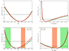 |
Fig. 5. SPLE parameters for the galaxy acting as main gravitational deflector to FBQ 0951+2635. The lines in green and red result from the astrometric constraints in APS 1 (see Table 2; Jakobsson et al. 2005) and APS 2 (see Table 2; Sluse et al. 2012a), respectively. Top left panel: Power-law index. Top right panel: True mass scale. Bottom left panel: Ellipticity of the mass distribution. Bottom right panel: Position angle of the mass distribution. Our solutions for e and θe are also compared with the observed (near-IR) morphology of the galaxy. The light green and light salmon rectangles represent 1σ intervals in APS 1 and APS 2, respectively. |
We showed that the SPLE-based reconstruction of the galaxy mass is very weakly affected by the difference between the image separation in APS 1 and APS 2. Moreover, despite discrepancies between the galaxy shape in these two datasets (∼6σ in eG and ∼3σ in θeG), when the formal errors are taken into account, the (eG, θeG) measurements are consistent with the (e, θe) solutions from the SPLE mass model (see Figure 5). Our lensing mass modelling focuses on the use of a Hubble constant that corresponds to an average of the main measurements from different experiments (H0 = 71 km s−1 Mpc−1; e.g., Di Valentino et al. 2021) and typical values of the constraints on secondary deflectors for this concordance H0. Therefore, when the current uncertainties in H0 and in the effects by secondary deflectors are taken into account, the error bars of αpl, b, e, and θe increase. As an example, a reasonable H0 interval of 68 to 74 km s−1 Mpc−1 (e.g., Di Valentino et al. 2021) increases the uncertainties in αpl by about 6.5%. These enlargements are similar to those associated with the errors in κext and γext (the error in θγext is not mentioned; Wilson et al. 2017), and they are clearly below the 18% uncertainties estimated for αpl.
We also considered the DV mass model and all (astrometric and morphological) constraints in APS 1 and APS 2. Interestingly, the DV mass distribution is reasonably consistent with the constraints in APS 2 (χ2∼ 3.7), suggesting that a constant mass-to-light ratio galaxy cannot be ruled out (see also Magain & Chantry 2013). The best-fit solution includes a true mass scale of 1 12 and reproduces the morphological measurements of Sluse et al. well (e = 0.45, θe = 13.0°, and R = 0
 78). However, using APS 1, we did not achieve a good solution for the lensing mass because χ2∼ 175 is much higher than the d.o.f. = 3 (see the end of Sect. 3.2). This high χ2 value is largely due to the morphological constraints in APS 1, and the main difference between the two light distributions of G lies in the effective radius: RG in APS 2 is larger by one order of magnitude than RG in APS 1.
To decide whether light is an acceptable tracer of the mass in the galaxy at a redshift of 0.26, we reanalysed the HST archival data of FBQ 0951+2635 with special attention to the value of the effective radius. The central idea was to repeat the evaluation of Jakobsson et al. of RG. These authors used a technique that was less refined than that of the COSmological MOnitoring of GRAvItational Lenses project (Sluse et al. 2012a). More specifically, we took the NICMOS drizzled frame in the H band and used the A image as an empirical point spread function (as in Jakobsson et al.), and then applied the IMFITFITS software (McLeod et al. 1998) by setting the positions of A and B at the values cited by Jakobsson et al. (2005). For a DV brightness profile, our approach yields an effective radius that is significantly larger than that estimated by Jakobsson et al. and is closer to the measurement of Sluse at al.. Jakobsson et al. most likely underestimated the effective radius, while the solution of Sluse et al. for RG relies on an iterative MCS deconvolution algorithm (Chantry & Magain 2007) and seems much more reliable. Hence, we cannot rule out a constant mass-to-light ratio DV model.
4. Conclusions
Prior to this work, optical, near-IR and radio observations towards the doubly imaged quasar FBQ 0951+2635 have provided a rich set of constraints for the gravitational lens system. However, unfortunately, early optical monitoring in the period 1999–2001 did not lead to a reliable time delay between the two quasar images (e.g., Jakobsson et al. 2005; Eulaers & Magain 2011; Rathna Kumar et al. 2015), which is a key constraint to blindly reconstruct the mass structure of the main lensing galaxy G, that is, its mass scale and morphology, or to be used for time-delay cosmography (e.g., Birrer et al. 2024). We focused on a robust determination of the time delay and discussed the structure of the non-local early-type galaxy G (e.g., Kochanek et al. 2000; Eigenbrod et al. 2007).
We considered new optical light curves in the period 2008–2024, including significant intrinsic fluctuations and consisting of quasar image magnitudes at 213 epochs. These GLENDAMA+ records were merged together with the early records, and we then used two different cross-correlation techniques to match the light curves of the two images by allowing for a time delay and microlensing polynomial variability. We also presented easy-to-use Python scripts associated with the two techniques and obtained a time delay of 13.5 ± 1.6 d (1σ confidence interval). This measurement is reliable up to ∼10% and resolves the long-standing controversy over the time delay of FBQ 0951+2635. In addition, a fifth-degree microlensing polynomial describes the long-timescale evolution of the difference light curve well. We also note that the current optical-passband flux ratio is close to the macro-magnification ratio.
Most previous reconstructions of the mass of G from a SPLE model were based on the assumption of isothermality (αpl = 1) and on priors on e and θe from the observed light structure (e.g., Sluse et al. 2012a). However, it is possible to blindly fit the parameters of the mass structure of G by knowing 1σ intervals for the positions of the quasar images and G, the macro-magnification ratio, and the time delay, along with typical values of the source and lens redshifts, the convergence and shear due to secondary gravitational deflectors, and the main cosmological parameters. For a SPLE mass model, hypotheses or priors on αpl, e and θe are not required. Additionally, the effective mass scale arising from the SPLE model fitting can be converted into a true mass scale of G. Thus, the constraints in Table 2 lead to SPLE mass solutions whose deviation from isothermality is consistent with studies of lensing galaxies selected from the SLACS Survey (Koopmans et al. 2006; Barnabè et al. 2009; Koopmans et al. 2009). As expected, the shapes of the mass and near-infrared light distributions of G also agree well (e.g., Koopmans et al. 2006). We also note that a DV mass model (constant mass-to-light ratio galaxy) cannot be ruled out based on the current data.
The observational constraints in Table 2 can be used for a more detailed study of the mass structure of G by considering models of the galaxy other than the SPLE and DV (e.g. Schneider & Sluse 2013; Kochanek 2020). For example, light-based priors on e and θe allow one to study mass models that incorporate two more parameters. New observations of the lens system will also contribute to a better understanding of the galaxy structure and will open the door to the analysis of its mass distribution based on accurate non-parametric reconstructions (e.g., Saha & Williams 1997; Diego et al. 2005). Future observations should include the spatially resolved stellar kinematics of G and a detailed imaging of the lensing galaxy and the lensed host galaxy of the quasar. In particular, new near-IR imaging along with dedicated analysis techniques are expected to definitively resolve the controversy about the light structure of the galaxy (Jakobsson et al. 2005; Sluse et al. 2012a; Rivera et al. 2023).
Data availability
Table 1 is available at the CDS via anonymous ftp to cdsarc.cds.unistra.fr (130.79.128.5) or via https://cdsarc.cds.unistra.fr/viz-bin/cat/J/A+A/694/A31
The mass scale is defined in Eq. (26) of Keeton (2002). For a singular isothermal sphere, it equals the Einstein radius.
Acknowledgments
The Liverpool Telescope (LT) is operated on the island of La Palma by Liverpool John Moores University in the Spanish Observatorio del Roque de los Muchachos of the Instituto de Astrofísica de Canarias with financial support from the UK Science and Technology Facilities Council. We thank the staff of the LT for a kind interaction. We also thank the anonymous referee for providing valuable feedback on the original manuscript. VNS acknowledges the Universidad de Cantabria (UC) and the Spanish Agencia Estatal de Investigacion (AEI) for financial support for a long stay at the UC in the period 2022–2024. This research has been supported by the grant PID2020-118990GB-I00 funded by MCIN/AEI/10.13039/501100011033.
References
- Abbott, T. M. C., Adamów, M., Aguena, M., et al. 2021, ApJS, 255, 20 [NASA ADS] [CrossRef] [Google Scholar]
- Barnabè, M., Czoske, O., Koopmans, L. V. E., et al. 2009, MNRAS, 399, 21 [CrossRef] [Google Scholar]
- Birrer, S., Shajib, A. J., Galan, A., et al. 2020, A&A, 643, A165 [NASA ADS] [CrossRef] [EDP Sciences] [Google Scholar]
- Birrer, S., Millon, M., Sluse, D., et al. 2024, Space Sci. Rev., 220, 48 [NASA ADS] [CrossRef] [Google Scholar]
- Capellari, M., Romanowsky, A. J., Brodie, J. P., et al. 2015, ApJ, 804, L21 [NASA ADS] [CrossRef] [Google Scholar]
- Chantry, V., & Magain, P. 2007, A&A, 470, 467 [NASA ADS] [CrossRef] [EDP Sciences] [Google Scholar]
- Di Valentino, E., Mena, O., Pan, S., et al. 2021, Class. Quant. Grav., 38, 153001 [NASA ADS] [CrossRef] [Google Scholar]
- Diego, J. M., Protopapas, P., Sandvik, H. B., & Tegmark, M. 2005, MNRAS, 360, 477 [Google Scholar]
- Eigenbrod, A., Courbin, F., & Meylan, G. 2007, A&A, 465, 51 [NASA ADS] [CrossRef] [EDP Sciences] [Google Scholar]
- Eulaers, E., & Magain, P. 2011, A&A, 536, A44 [NASA ADS] [CrossRef] [EDP Sciences] [Google Scholar]
- Fadely, R., Keeton, C. R., Nakajima, R., & Bernstein, G. M. 2010, ApJ, 711, 246 [Google Scholar]
- Falco, E. E., Gorenstein, M. V., & Shapiro, I. I. 1985, ApJ, 289, L1 [Google Scholar]
- Fian, C., Mediavilla, E., Motta, V., et al. 2021, A&A, 653, A109 [NASA ADS] [CrossRef] [EDP Sciences] [Google Scholar]
- Flewelling, H. A., Magnier, E. A., Chambers, K. C., et al. 2020, ApJS, 251, 7 [NASA ADS] [CrossRef] [Google Scholar]
- Gil-Merino, R., Goicoechea, L. J., Shalyapin, V. N., & Oscoz, A. 2018, A&A, 616, A118 [NASA ADS] [CrossRef] [EDP Sciences] [Google Scholar]
- Goicoechea, L. J., & Shalyapin, V. N. 2016, A&A, 596, A77 [NASA ADS] [CrossRef] [EDP Sciences] [Google Scholar]
- Grogin, N. A., & Narayan, R. 1996, ApJ, 464, 92 [NASA ADS] [CrossRef] [Google Scholar]
- Hinshaw, G., Weiland, J. L., Hill, R. S., et al. 2009, ApJS, 180, 225 [Google Scholar]
- Jakobsson, P., Hjorth, J., Burud, I., et al. 2005, A&A, 431, 103 [NASA ADS] [CrossRef] [EDP Sciences] [Google Scholar]
- Keeton, C. R. 2001, arXiv e-prints [arXiv:astro-ph/0102340v1] [Google Scholar]
- Keeton, C. R. 2002, arXiv e-prints [arXiv:astro-ph/0102341v2] [Google Scholar]
- Kochanek, C. S. 2020, MNRAS, 493, 1725 [NASA ADS] [CrossRef] [Google Scholar]
- Kochanek, C. S., Falco, E. E., Impey, C. D., et al. 2000, ApJ, 543, 131 [NASA ADS] [CrossRef] [Google Scholar]
- Komatsu, E., Dunkley, J., Nolta, M. R., et al. 2009, ApJS, 180, 330 [NASA ADS] [CrossRef] [Google Scholar]
- Koopmans, L. V. E., Treu, T., Bolton, A. S., Burles, S., & Moustakas, L. A. 2006, ApJ, 649, 599 [Google Scholar]
- Koopmans, L. V. E., Bolton, A., Treu, T., et al. 2009, ApJ, 703, L51 [NASA ADS] [CrossRef] [Google Scholar]
- Magain, P., & Chantry, V. 2013, arXiv e-prints [arXiv:1303.6896v1] [Google Scholar]
- McLeod, B. A., Bernstein, G. M., Rieke, M. J., & Weedman, D. W. 1998, AJ, 115, 1377 [NASA ADS] [CrossRef] [Google Scholar]
- Metcalf, R. B., & Madau, P. 2001, ApJ, 563, 9 [NASA ADS] [CrossRef] [Google Scholar]
- Millon, M., Courbin, F., Bonvin, V., et al. 2020a, A&A, 640, A105 [NASA ADS] [CrossRef] [EDP Sciences] [Google Scholar]
- Millon, M., Galan, A., Courbin, F., et al. 2020b, A&A, 639, A101 [NASA ADS] [CrossRef] [EDP Sciences] [Google Scholar]
- Momcheva, I. G., Williams, K. A., Cool, R. J., Keeton, C. R., & Zabludoff, A. I. 2015, ApJS, 219, 29 [NASA ADS] [CrossRef] [Google Scholar]
- Moustakas, L. A., & Metcalf, R. B. 2003, MNRAS, 339, 607 [NASA ADS] [CrossRef] [Google Scholar]
- Paraficz, D., Hjorth, J., Burud, I., Jakobsson, P., & Elíasdóttir, Á. 2006, A&A, 455, L1 [NASA ADS] [CrossRef] [EDP Sciences] [Google Scholar]
- Pelt, J., Kayser, R., Refsdal, S., & Schramm, T. 1996, A&A, 305, 97 [NASA ADS] [Google Scholar]
- Planck Collaboration VI. 2020, A&A, 641, A6 [NASA ADS] [CrossRef] [EDP Sciences] [Google Scholar]
- Rathna Kumar, S., Stalin, C. S., & Prabhu, T. P. 2015, A&A, 580, A38 [NASA ADS] [CrossRef] [EDP Sciences] [Google Scholar]
- Refsdal, S. 1964, MNRAS, 128, 307 [NASA ADS] [CrossRef] [Google Scholar]
- Rivera, A. B., Morgan, C. W., Florence, S. M., et al. 2023, ApJ, 952, 54 [NASA ADS] [CrossRef] [Google Scholar]
- Rusu, C. E., Fassnacht, C. D., Sluse, D., et al. 2017, MNRAS, 467, 4220 [NASA ADS] [CrossRef] [Google Scholar]
- Saha, P., & Williams, L. L. R. 1997, MNRAS, 292, 148 [NASA ADS] [CrossRef] [Google Scholar]
- Schechter, P. L., Gregg, M. D., Becker, R. H., Helfand, D. J., & White, R. L. 1998, AJ, 115, 1371 [NASA ADS] [CrossRef] [Google Scholar]
- Schneider, P., & Sluse, D. 2013, A&A, 559, A37 [NASA ADS] [CrossRef] [EDP Sciences] [Google Scholar]
- Shajib, A. J., Birrer, S., Treu, T., et al. 2019, MNRAS, 483, 5649 [Google Scholar]
- Shajib, A. J., Mozumdar, P., Cheng, G. C.-F., et al. 2023, A&A, 673, A9 [NASA ADS] [CrossRef] [EDP Sciences] [Google Scholar]
- Shajib, A. J., Vernardos, G., Collett, T. E., et al. 2024, Space Sci. Rev., 220, 87 [CrossRef] [Google Scholar]
- Shalyapin, V. N., & Goicoechea, L. J. 2017, ApJ, 836, 14 [NASA ADS] [CrossRef] [Google Scholar]
- Shalyapin, V. N., Goicoechea, L. J., Koptelova, E., et al. 2009, MNRAS, 397, 1982 [NASA ADS] [CrossRef] [Google Scholar]
- Sheu, W., Shajib, A. J., Treu, T., et al. 2024, arXiv e-prints [arXiv:2408.10316] [Google Scholar]
- Sluse, D., Chantry, V., Magain, P., Courbin, F., & Meylan, G. 2012a, A&A, 538, A99 [NASA ADS] [CrossRef] [EDP Sciences] [Google Scholar]
- Sluse, D., Hutsemékers, D., Courbin, F., Meylan, G., & Wambsganss, J. 2012b, A&A, 544, A62 [NASA ADS] [CrossRef] [EDP Sciences] [Google Scholar]
- Suyu, S. H., Marshall, P. J., Auger, M. W., et al. 2010, ApJ, 711, 201 [Google Scholar]
- Suyu, S. H., Auger, M. W., Hilbert, S., et al. 2013, ApJ, 766, 70 [Google Scholar]
- Suyu, S. H., Treu, T., Hilbert, S., et al. 2014, ApJ, 788, L35 [NASA ADS] [CrossRef] [Google Scholar]
- Suyu, S. H., Chang, T.-C., Courbin, F., & Okumura, T. 2018, Space Sci. Rev., 214, 91 [NASA ADS] [CrossRef] [Google Scholar]
- Tewes, M., Courbin, F., & Meylan, G. 2013, A&A, 553, A120 [NASA ADS] [CrossRef] [EDP Sciences] [Google Scholar]
- Tie, S. S., & Kochanek, C. S. 2018, MNRAS, 473, 80 [Google Scholar]
- Treu, T., & Marshall, P. J. 2016, A&ARv, 24, 11 [Google Scholar]
- Wang, Y., Vogelsberger, M., Xu, D., et al. 2020, MNRAS, 491, 5188 [Google Scholar]
- Wilson, M. L., Zabludoff, A. I., Keeton, C. R., et al. 2017, ApJ, 850, 94 [NASA ADS] [CrossRef] [Google Scholar]
- Wong, K. C., Suyu, S. H., Cheng, G. C.-F., et al. 2020, MNRAS, 498, 1420 [NASA ADS] [CrossRef] [Google Scholar]
Appendix A: Easy-to-use software for time delay estimation in presence of microlensing
We consider a double quasar with images A and B. The A image magnitudes at observing times ti (i = 1, …, NA) are given by Ai = mA(ti), whereas Bj = mB(tj) at observing times tj (j = 1, …, NB) represent the light curve of B. The A image data are shifted by a time lag τ and a microlensing polynomial of degree Nml, and then compared to the B image data. The microlensing polynomial
 (A.1)
(A.1)
is characterised by coefficients ak (k = 0, …, Nml), and the central idea is to find the values of (τ, ak) that provide the best match between the shifted light curve of A and the original light curve of B.
To estimate best values of (τ, ak), we minimise two different merit functions: dispersion D42 and reduced chi-square χr2 (see main text and here below). Two main advantages of using a polynomial function to account for the microlensing variability are the possibility to describe a very general behaviour and the linear role of polynomial coefficients in merit functions. Thus, for each value of τ, we can optimise the linear parameters ak analytically, so multivariable merit functions are reduced to 1D spectra depending on the non-linear parameter τ. Minima of these 1D spectra yield estimates of the time delay between A and B. We also note that Python scripts to use both techniques (merit functions) are available at the GitHub repository URL https://github.com/glendama/q0951time_delay, and draw attention to the fact that the so-called polynomial order in the scripts (Nord) equals Nml + 1.
A.1. Minimum dispersion method
The merit function is given by
![Mathematical equation: $$ \begin{aligned} D^2_4(\tau , a_k) = \frac{\sum _i \sum _j W_{ij} S_{ij}[A_i - B_j + P(t_i)]^2}{\sum _i \sum _j W_{ij} S_{ij}} , \end{aligned} $$](/articles/aa/full_html/2025/02/aa52234-24/aa52234-24-eq6.gif) (A.2)
(A.2)
where Wij = 1/(σAi2 + σBj2) are statistical weights computed from photometric errors and Sij = exp[−(ti − tj + τ)2/β2] are weights for time separations. Our time-separation weighting scheme relies on a Gaussian function and a "decorrelation length" β, and it is inspired by Eq. (13) of Pelt et al. (1996).
For each value of τ, the minimisation of the dispersion with respect to the polynomial coefficients, i.e., ∂D42/∂ak = 0, produces the system of linear equations
 (A.3)
(A.3)
This system of Nml + 1 equations can be solved by standard procedures of linear algebra, yielding a set of optimal microlensing coefficients ak for each time lag and the corresponding dispersion spectrum D42(τ).
A.2. Reduced chi-square minimisation
The merit function has the form
![Mathematical equation: $$ \begin{aligned} \chi ^2_{\rm r}(\tau , a_k) = \frac{1}{N_{\rm {pair}} - (N_{\rm {ml}} + 2)} \sum _i W_i [A_i - B^{\prime }_i + P(t_i)]^2 , \end{aligned} $$](/articles/aa/full_html/2025/02/aa52234-24/aa52234-24-eq8.gif) (A.4)
(A.4)
where B′i is the B image magnitude binned around ti + τ to build the (Ai, B′i) pair, Npair is the total number of AB′ pairs for the time lag τ (i = 1, …, Npair), and Wi = 1/(σAi2 + σB′i2) is the inverse of the sum of squared uncertainties. To build the bin in B around ti + τ, we use a linear weighting function 1 − |ti − tj + τ|/α for dates tj verifying |ti − tj + τ|≤α.
The minimisation with respect to the microlensing coefficients ak yields the linear system
 (A.5)
(A.5)
and thus optimal values of ak for each time lag and the 1D spectrum χr2(τ).
All Tables
All Figures
|
Fig. 1. GLENDAMA+ light curves of FBQ 0951+2635. These new variability records mainly consist of photometric data from the LT (circles) and KST (squares), but also incorporate information provided by the PS (inverted triangles) and DES (triangles) databases. See main text for details. |
| In the text | |
|
Fig. 2. Time-delay estimation from the dispersion technique. The dispersion spectra D42 are based on a Gaussian weighting function whose width is described by the parameter β, as well as a fifth-degree microlensing polynomial (Nml = 5; see main text). Top panel: D42 spectra using the NOT light curves plus the new GLENDAMA+ brightness records and five values of β. These spectra have minima at time lags τ = 13–15 d. Bottom panel: 1σ confidence intervals for the time delay using 1000 synthetic light curves of each image and a large set of β values. A combined measurement from the six delay intervals for β = 4–9 d is highlighted with a light grey rectangle encompassing the individual measurements. |
| In the text | |
|
Fig. 3. Time-delay estimation from the χr2 technique and 1000 synthetic light curves of each quasar image. To match the light curves of the two images, a fifth-degree microlensing polynomial and binned light curves of B were considered, where bins of the B image have a semi-size α. The error bars represent 1σ confidence intervals for the time delay, and the black outlined rectangle contains five anomalous measurements (see main text). |
| In the text | |
|
Fig. 4. New 25 yr DLC of FBQ 0951+2635 in the red optical passbands from NOT-MT and GLENDAMA+ data. We also show solutions of the fifth-degree microlensing polynomial (thick solid line; see main text for details). For comparison purposes, we include the magnitude differences from VLA data (horizontal dash-dotted line; Jakobsson et al. 2005) and emission lines (horizontal dashed line; see Sect. 3.1). The striped rectangles represent the uncertainties in these two differences. |
| In the text | |
|
Fig. 5. SPLE parameters for the galaxy acting as main gravitational deflector to FBQ 0951+2635. The lines in green and red result from the astrometric constraints in APS 1 (see Table 2; Jakobsson et al. 2005) and APS 2 (see Table 2; Sluse et al. 2012a), respectively. Top left panel: Power-law index. Top right panel: True mass scale. Bottom left panel: Ellipticity of the mass distribution. Bottom right panel: Position angle of the mass distribution. Our solutions for e and θe are also compared with the observed (near-IR) morphology of the galaxy. The light green and light salmon rectangles represent 1σ intervals in APS 1 and APS 2, respectively. |
| In the text | |
Current usage metrics show cumulative count of Article Views (full-text article views including HTML views, PDF and ePub downloads, according to the available data) and Abstracts Views on Vision4Press platform.
Data correspond to usage on the plateform after 2015. The current usage metrics is available 48-96 hours after online publication and is updated daily on week days.
Initial download of the metrics may take a while.