| Issue |
A&A
Volume 694, February 2025
|
|
|---|---|---|
| Article Number | A191 | |
| Number of page(s) | 10 | |
| Section | Numerical methods and codes | |
| DOI | https://doi.org/10.1051/0004-6361/202451459 | |
| Published online | 12 February 2025 | |
Hybrid simulation method for agglomerate evolution in driven granular gases
University of Duisburg-Essen,
Lotharstr. 1,
47057
Duisburg,
Germany
★ Corresponding author; This email address is being protected from spambots. You need JavaScript enabled to view it.
Received:
11
July
2024
Accepted:
20
December
2024
Abstract
Aims. We present a new hybrid simulation method for protoplanetary dust evolution that is efficient and takes into account the complex fragmentation and agglomeration dynamics. We applied it to simulate the evolution of agglomerate size distributions for turbulent, charged systems.
Methods. The hybrid method combines kinetic Monte Carlo and discrete element simulations in such a way that the expensive latter is only deployed when two agglomerates collide. This method can easily be extended to include additional driving mechanisms, interactions, and the effects of inhomogeneities.
Results. Our simulations reveal an emerging steady state in the size distribution. Due to the efficiency of our method, we are able to extend previous results with improved statistics for the size distribution of large agglomerates; in addition to the previously reported power law, we find a regime with an exponential decay.
Key words: methods: numerical / planets and satellites: formation / protoplanetary disks / zodiacal dust
© The Authors 2025
 Open Access article, published by EDP Sciences, under the terms of the Creative Commons Attribution License (https://creativecommons.org/licenses/by/4.0), which permits unrestricted use, distribution, and reproduction in any medium, provided the original work is properly cited.
This article is published in open access under the Subscribe to Open model. This email address is being protected from spambots. You need JavaScript enabled to view it. to support open access publication.
1 Introduction
Undeniably, a process exists that leads to the formation of planets. The common conception is that this process starts with the agglomeration of micrometre-sized dust grains within protoplanetary disks, which stick because of cohesive contact forces. However, many studies came to the conclusion that growth should not continue beyond sizes of millimetres to metres, based on our current understanding of agglomerate stability and dust migration. For example, the bouncing barrier is a consequence of increasingly elastic collisions at lower collision velocities (see Dominik & Tielens 1997; Tanaka et al. 2012; Zsom et al. 2010 and a comprehensive review by Birnstiel et al. 2016), while the metre-size barrier limits growth because of rapid inward drift and the depletion of solids (Weidenschilling 1977; Nakagawa et al. 1986). In addition to these theoretical and numerical studies, the bouncing barrier was also observed in a number of microgravity experiments (Blum & Wurm 2008; Weidling et al. 2009; Güttler et al. 2010; Kelling et al. 2014; Demirci et al. 2017).
Mechanisms that help overcome growth barriers have been discussed, such as streaming instabilities and pressure bumps (e.g. Youdin & Goodman 2005; Simon et al. 2016; Squire & Hopkins 2018; Pinilla et al. 2012), but additional processes may be at play. One such mechanism that is suggested to aid growth past the bouncing barrier is the attraction of grains due to electrical charging, mainly through the triboelectric effect (contact electrification). Recent studies have found that charged particles compose significantly more stable agglomerates (Ruan & Li 2022) and increase the likelihood of larger agglomerates (Steinpilz et al. 2020; Singh & Mazza 2018). Notably, even though Steinpilz et al. (2020) and Singh & Mazza (2018) studied the agglomerate size distribution (ASD) in different setups, both recovered a power-law distribution with approximately the same exponent.
To find the crucial mechanisms in early-stage planet formation within systems similar to protoplanetary disks, that is, very dilute and driven granular gases, a new approach to simulations is necessary. Previous methods can be roughly separated into two categories, which suffer from different shortcomings:
First, there are probabilistic simulations as performed by, for example, Birnstiel et al. (2010), Johansen et al. (2008), Estrada et al. (2016), and Zsom et al. (2010). These simulations typically feature a very detailed description of the disk parameters that influence agglomerate growth. However, the collisions themselves, an integral part of the growth process, are only described by the purely probabilistic Smoluchowski equation. Specifically, coagulation and fragmentation behaviour is governed by the kernel functions used in these simulations. Thus, the choice of kernels has a strong impact on the results, and any kernel of reasonable complexity can only represent the actual collision in an extremely simplified way – even before one tries to include electrostatic interactions, as done by, for example, Ivlev et al. (2002) and Okuzumi et al. (2011).
Second, in complete contrast, there are discrete element method (DEM) simulations of granular gases, for example, Steinpilz et al. (2020) and Singh & Mazza (2018). While agglomerate-agglomerate collisions are calculated in detail, it is practically impossible, or at least extremely inefficient, to implement an environment that resembles a protoplanetary disk. To understand why this is the case, consider the following: at typical particle densities, the mean free path of agglomerates is very long; consequently, the ASD evolution takes place on timescales longer than years. On the other hand, particle–particle interactions take place on timescales of nanoseconds. Therefore, the overwhelming majority of the simulation time is occupied by dynamics that do not need to be resolved by a DEM code; only for the collisions themselves is it mandatory. Putting the above into numbers, at a reasonable time step size of 10−6 s, simulating the evolution of just one year would take roughly 1013 time steps – an impossible amount considering that each step will include expensive computations. Another important shortcoming of the previous DEM studies is that only freely cooling systems were considered. The granular gas in a protoplanetary disk, however, is driven by a number of mechanisms, for example hydrodynamics and gravity.
Based on these considerations, we propose a novel hybrid method for ASD evolution simulations in which we use a kinetic Monte Carlo approach for the time evolution between two collisions. This is the natural probabilistic partner to the deterministic DEM because together they describe a specific trajectory across the disparate timescales. Even though kinetic Monte Carlo simulations could describe multi-agglomerate collisions, for a dilute granular gas it is justified to only consider binary collisions. Furthermore, since all other particles are very far away, the influence of any long-range interaction is negligible compared with the interactions between the collision partners themselves. Additionally, the coupling to an external driving mechanism, in the present case the coupling to the turbulent gas, is assumed to be strong enough to allow us to neglect long-range interactions for almost the whole time between collisions, removing the need to take into account corresponding correlations between agglomerates. Therefore, the hybrid method requires the granular gas to be sufficiently diluted such that the time between collisions exceeds the characteristic coupling time.
These assumptions allow for iterative simulations of binary collisions, which have low computational costs as the particle number and simulated times are relatively low and short, respectively. A code that is able to reproduce the results presented in Sect. 3 is publicly available1.
2 Methods
The hybrid method described in this work focuses on the agglomeration behaviour of charged particles; the general concept is applicable to all kinds of interactions. In fact, only considering short-range interactions (e.g. adhesion) would simplify the method. The following description should be viewed as a blueprint; the details (interactions, driving mechanisms, modifications to collision rates etc.) may be altered to suit the needs for a plethora of disk models. This alteration would be simple, compared with changing a regular DEM simulation, as many processes only influence the setup for a collision, but not the actual particle dynamics during a collision. For example, including sedimentation as a driving mechanism would only change the formula used to calculate the relative velocities, discussed in Sect. 2.1.4.
2.1 Reducing granular gas dynamics to binary collisions
Using this method, we simulated the evolution of a population of agglomerates in a representative volume element of some region in the protoplanetary disk. From this population, we randomly chose two agglomerates for collision. The agglomerates resulting from the detailed simulation of this collision, whose numbers can possibly range anywhere from one (perfect merger of the collision partners) to the number of particles making up the collision partners (complete pulverisation), replace their parent agglomerates in the population. Then, the next agglomerate pair is chosen.
Each agglomerate consists of particles at certain coordinates with velocities, angular velocities (all in the agglomerate’s centre of mass coordinate system) and fixed charges in their centres. Hence, even two agglomerates of the same mass may drastically differ in porosity, shape, total charge etc.
As agglomerates can stick together in a collision, the number of agglomerates within the population may decrease. To prevent finite size effects, the population is self-duplicated (and the representative volume element accordingly becomes twice as big) every time it reaches half of its original size; therefore, also a population of half the original size must be a representative sample of the agglomerate distribution in the system we are looking to describe. This method was introduced by Liffman (1992, termed ‘topping up’) and further developed into the constant-N algorithm by Smith & Matsoukas (1998), which has been used to study agglomerate size evolution in protoplanetary disks (e.g. Ormel et al. 2007). In this work, however, we used Liffman’s topping up algorithm, as we do not know how sensitive the size evolution is with regard to changes to the size distribution (the fact that topping up does not alter the shape of the distribution is a key difference compared with the constant-N algorithm).
It should be noted that we use the term ‘agglomerate’ to also include monomers, special agglomerates that only consist of a single particle. When we use the term ‘particle’, however, we are referring to a primary particle, irrespective of what kind of agglomerate it might be a part of.
2.1.1 Macroscopic time
By the nature of this hybrid simulation technique, the time evolution of all results is given through the number of collisions that have occurred until a certain point. In general kinetic Monte Carlo terms, the collisions are events with given rates of occurrence; the overall theory is applicable to all kinds of such events (see e.g. Young & Elcock 1966 and Jansen 2012).
To convert the number of collisions into a real, physical time, each realised collision has to be associated with a waiting time δt, that is, the time between the previous and the current collision. It is distributed according to an exponential probability density function,
![Mathematical equation: $\[f(\delta t)=\frac{1}{\langle\delta t\rangle} \exp \left(\frac{\delta t}{\langle\delta t\rangle}\right),\]$](/articles/aa/full_html/2025/02/aa51459-24/aa51459-24-eq1.png) (1)
(1)
where the average ⟨δt⟩ is the inverse of the sum of the rates for all possible collisions in the current state of the population. Assuming homogeneity within the simulated representative volume element V, the number density of each individual agglomerate is 1/V. Therefore, given the relative velocity vij and the collision cross-section σcol,ij, we write the rate for the collision of an agglomerate i with a specific other agglomerate j as
![Mathematical equation: $\[\Omega_{i j}=\frac{\sigma_{\mathrm{col}, i j} v_{i j}}{V}.\]$](/articles/aa/full_html/2025/02/aa51459-24/aa51459-24-eq2.png) (2)
(2)
How big is the representative volume element for a given mass of solids ms? In our simulation, all N particles have the same mass, m, so that ms = N m. Within the scope of this paper, we assumed a fixed mass ratio of gas to solids β := mg/ms = 100 (e.g. Draine et al. 2007). Let ϱg = mg/Vg be the gas density, where we can neglect the volume of the solids to write Vg ≈ V. Thus, we find the volume, V, in dependence of the total mass of solids,
![Mathematical equation: $\[\begin{equation*}V=\frac{\beta m_{\mathrm{s}}}{\varrho_{\mathrm{g}}},\end{equation*}\]$](/articles/aa/full_html/2025/02/aa51459-24/aa51459-24-eq3.png) (3)
(3)
and, consequently, the average waiting time as
![Mathematical equation: $\[\langle\delta t\rangle=\frac{V}{\sum_{i>j} \sigma_{\mathrm{col}, i j} v_{i j}}=\beta \frac{m}{\varrho_{\mathrm{g}}} \frac{N}{\sum_{i>j} \sigma_{\mathrm{col}, i j} v_{i j}},\]$](/articles/aa/full_html/2025/02/aa51459-24/aa51459-24-eq4.png) (4)
(4)
where the summation takes all possible collisions into account exactly once. As these rates generally change (and are recomputed) after each collision, the mean of the waiting time distribution f(δt) is not constant. Following this discussion, we can now identify the time of a specific collision as the sum of all previously sampled waiting times, δt.
2.1.2 Collision probability
Based on the results from the previous section,
![Mathematical equation: $\[P_{i j}=\Omega_{i j}\langle\delta t\rangle\]$](/articles/aa/full_html/2025/02/aa51459-24/aa51459-24-eq5.png) (5)
(5)
is the probability that agglomerates i and j collide in the time span ⟨δt⟩, given that a single collision occurs (we assumed that the collision probabilities are so small that higher orders [multiple collisions] are unimportant).
As Coulomb interactions between different agglomerates are negligible compared with the coupling to the gas for the majority of the time between two collisions, we assume that they have no significant impact on the relative velocity in the collision rate – an assumption that does not hold for the collision cross-section. Neglecting higher order terms, the collision cross-section of two charged spheres with radii ρ1 and ρ2, a reduced mass,
![Mathematical equation: $\[M_{\mathrm{red}}=\frac{M_{1} M_{2}}{M_{1}+M_{2}},\]$](/articles/aa/full_html/2025/02/aa51459-24/aa51459-24-eq6.png) (6)
(6)
and charges Q1 and Q2 is given independently by Ivlev et al. (2002) and Scheffler & Wolf (2002) as
![Mathematical equation: $\[\sigma_{\mathrm{col}}=\pi\left(\rho_{1}+\rho_{2}\right)^{2}\left(1-\frac{Q_{1} Q_{2}}{\rho_{1}+\rho_{2}} \frac{2}{M_{\mathrm{red}} v^{2}}\right).\]$](/articles/aa/full_html/2025/02/aa51459-24/aa51459-24-eq7.png) (7)
(7)
For non-spherical agglomerates, the radii ρ1 and ρ2 in the collision cross-section must be given by the maximal extent of the agglomerates, measured from the centre of mass. This is because, for anything less, the collision probability would not account for collisions with the maximum possible distance between the centres of mass. On the other hand, it is no problematic overestimation of the collision probability either, since it is still possible that the agglomerates do not collide in the DEM simulation. Therefore, this hybrid ansatz allows for the splitting of the collision probability into a trivial part (Eq. (7)) and a non-trivial part, which is directly resolved within the DEM simulation. The only drawback is that some unnecessary simulations are performed, that is, simulations in which the agglomerates do not come into contact, increasing the computation time. This is, however, a small price to pay with respect to the substantial benefits of this approach (i.e. not having to calculate all particle trajectories all the time for more than 1013 time steps).
2.1.3 Setup of imminent collisions
A number of quantities influence the initial setup for each collision. These are the initial distance between the agglomerates, their initial relative centre of mass velocity, the impact parameter, as well as their orientations.
The initial distance dinit determines the initial potential energy of the collision partners and, thus, has a direct relation to the impact velocities, as explained below. In the simulation, the distance is calculated as the maximal extent from the centre of mass of the larger agglomerate times a parameter, the initial distance coefficient, chosen to be 10 in the current work.
As long as dinit is chosen to be large enough that electrical dipoles and higher orders are negligible, the consequences of this choice can be absorbed into the initial relative velocity: for a (Coulomb interaction free) relative velocity v, the reduced mass mred as well as the agglomerate charges Q1 and Q2, the initial velocity at distance dinit is given by
![Mathematical equation: $\[v_{\text {init }}=\sqrt{v^{2}-2 \frac{Q_{1} Q_{2}}{M_{\text {red}} d_{\text {init}}}}.\]$](/articles/aa/full_html/2025/02/aa51459-24/aa51459-24-eq8.png) (8)
(8)
In other words, the relative velocity can be split into a free relative velocity v, that is, the relative velocity in the absence of electrical charges, and the velocity change by converting potential energy from the distance travelled in the electric potential to kinetic energy.
Obviously, if the free relative velocity is too small to overcome the Coulomb barrier between two charged agglomerates of equal polarity, a collision is not possible at all. In this case, the respective collision probability is zero.
The simulation draws a random impact parameter b ∈ [0, bmax] for each collision from the probability density function ![Mathematical equation: $\[2 b / b_{\text {max }}^{2}\]$](/articles/aa/full_html/2025/02/aa51459-24/aa51459-24-eq9.png) , accounting for the fact that larger impact parameters are more likely in three dimensions. Using the simplest estimate, the simulation determines the maximum possible impact parameter from the collision cross-section as
, accounting for the fact that larger impact parameters are more likely in three dimensions. Using the simplest estimate, the simulation determines the maximum possible impact parameter from the collision cross-section as ![Mathematical equation: $\[b_{\max }=\sqrt{\sigma_{\mathrm{col}} / \pi}.\]$](/articles/aa/full_html/2025/02/aa51459-24/aa51459-24-eq10.png) .
.
The two agglomerates are initialised with random orientations. Their angular momenta follow from the particles’ positions and velocities. The initial population consists of dimers with random orientations and no angular momenta.
Even though all dynamical variables of the particles, including velocities, are kept between collisions, there will never be any significant amount of internal kinetic energy left from the last collision when two agglomerates make contact. This is because the dissipation timescales of the contact interactions are orders of magnitude shorter than dinit/vinit.
2.1.4 Relative velocities in a turbulent gas
An agglomerate of mass M couples via friction to the gas, which is present in a protoplanetary disk, with a characteristic stopping time
![Mathematical equation: $\[\tau_{\mathrm{s}}=\frac{3 M}{4 v_{\text {th}} \varrho_{\mathrm{g}} \sigma_{\text {aer}}}.\]$](/articles/aa/full_html/2025/02/aa51459-24/aa51459-24-eq11.png) (9)
(9)
Here, σaer is the aerodynamic cross-section, vth the thermal gas velocity and ϱg the gas mass density (Ormel & Cuzzi 2007). The stopping time is related to the dimensionless Stokes number St = τs/tL, where tL is the orbital period, which we chose to be one year.
The aerodynamic (geometric) cross-section needed for the stopping time is a complicated quantity. Even assuming molecular free flow, which will break down for agglomerate sizes above centimetres (Weidenschilling & Cuzzi 1993), and instantaneous orientation of the agglomerates with respect to the gas flow, a unique orientation and, thus, a unique cross-section generally does not exist. To keep the approach simple, we used the radius of gyration to approximate the aerodynamic cross-section ![Mathematical equation: $\[\sigma_{\text {aer }}=\pi \rho_{\mathrm{gyr}}^{2}\]$](/articles/aa/full_html/2025/02/aa51459-24/aa51459-24-eq12.png) . With the mass density ϱagg(r) of an agglomerate that has its centre of mass in the coordinate origin, the radius of gyration is given as
. With the mass density ϱagg(r) of an agglomerate that has its centre of mass in the coordinate origin, the radius of gyration is given as
![Mathematical equation: $\[\rho_{\mathrm{gyr}}=\sqrt{\frac{1}{M} \int_{\mathbb{R}^{3}} \mathrm{~d}^{3} r ~\boldsymbol{r}^{2} \varrho_{\mathrm{agg}}(\boldsymbol{r})}.\]$](/articles/aa/full_html/2025/02/aa51459-24/aa51459-24-eq13.png) (10)
(10)
In the following, we discuss the model for turbulence-induced relative velocities, which greatly exceed the thermal, sedimentation and radial drift velocities (Blum et al. 1996). Here, the Reynolds number Re = 2.32 · 107 and the velocity vg = 18.5 m/s, which relates to the total kinetic energy of all eddies (see Eq. (2) in Ormel & Cuzzi 2007 and Eq. (46) in Birnstiel et al. 2011) characterise the turbulence. These values correspond to a turbulence strength of α = 10−4 (Weidenschilling & Cuzzi 1993).
The average squared relative velocity of two agglomerates (Δv)2 := ⟨(v1 – v2)2⟩ is given by Ormel & Cuzzi (2007) as
![Mathematical equation: $\[(\Delta v)^{2}=\sum_{i \in\{1,2\}} v_{\mathrm{g}}^{2}\left(1-G_{i}^{(1)}-G_{i}^{(2)} G_{i}^{(3)}\right),\]$](/articles/aa/full_html/2025/02/aa51459-24/aa51459-24-eq14.png) (11)
(11)
with the abbreviations
![Mathematical equation: $\[G_{i}^{(1)}:=\frac{\mathrm{St}_{i}^{2}\left(1-\mathrm{Re}^{-1 / 2}\right)}{\left(\mathrm{St}_{i}+1\right)\left(\mathrm{St}_{i}+\mathrm{Re}^{-1 / 2}\right)},\]$](/articles/aa/full_html/2025/02/aa51459-24/aa51459-24-eq15.png) (12)
(12)
![Mathematical equation: $\[G_{i}^{(2)}:=\frac{2 \tau_{\mathrm{s}, i}}{\tau_{\mathrm{s}, 1}+\tau_{\mathrm{s}, 2}},\]$](/articles/aa/full_html/2025/02/aa51459-24/aa51459-24-eq16.png) (13)
(13)
and
![Mathematical equation: $\[\begin{align*}G_{i}^{(3)}:= & ~1-\left(\frac{k^{*}}{k_{\min }}\right)^{-2 / 3}-\frac{\mathrm{St}_{i}}{1+\mathrm{St}_{i}}\\& +\frac{\mathrm{St}_{i}}{1+\mathrm{St}_{i}\left(k^{*} / k_{\min }\right)^{2 / 3}}.\end{align*}\]$](/articles/aa/full_html/2025/02/aa51459-24/aa51459-24-eq17.png) (14)
(14)
Here, we use the index i ∈ {1, 2} to distinguish the values of the Stokes numbers and the stopping times of the two agglomerates considered as collision partners. The lowest wavenumber kmin is given by the inverse size of the largest eddy.
Furthermore, we need to discuss the wavenumber k*. It is given by ![Mathematical equation: $\[k^{*}=\min\{k_{1}^{*}, k_{2}^{*}\}\]$](/articles/aa/full_html/2025/02/aa51459-24/aa51459-24-eq18.png) , where the wavenumber
, where the wavenumber ![Mathematical equation: $\[k_{i}^{*}\]$](/articles/aa/full_html/2025/02/aa51459-24/aa51459-24-eq19.png) is the separation between two classes of eddies with respect to agglomerate i (see Völk et al. 1980):
is the separation between two classes of eddies with respect to agglomerate i (see Völk et al. 1980):
| Class I eddies | are slow and large enough that the agglomerate forgets its initial velocity and fully couples to the eddy, and |
| Class II eddies | are fast and small enough that the influence on the agglomerate’s initial velocity is merely that of a small perturbation. |
Every agglomerate couples differently to the eddies, so this separation wavenumber also varies for different agglomerates. Importantly, the above formula, Eq. (11), is only defined for not too massive agglomerates, that is, only for agglomerates with τs < tL, as the product ![Mathematical equation: $\[$G_{i}^{(2)} G_{i}^{(3)}$\]$](/articles/aa/full_html/2025/02/aa51459-24/aa51459-24-eq20.png) (the velocity correlation term) would be zero otherwise (k* = kmin). This is because all eddies could then be considered as class II eddies, which practically removes velocity correlations. Conversely, k*/kmin has the upper bound kmax/kmin = Re3/4, for which all eddies are of class I. The highest wavenumber kmax is determined by the Kolmogorov scale. Ormel & Cuzzi (2007) give
(the velocity correlation term) would be zero otherwise (k* = kmin). This is because all eddies could then be considered as class II eddies, which practically removes velocity correlations. Conversely, k*/kmin has the upper bound kmax/kmin = Re3/4, for which all eddies are of class I. The highest wavenumber kmax is determined by the Kolmogorov scale. Ormel & Cuzzi (2007) give
![Mathematical equation: $\[\frac{k_{i}^{*}}{k_{\min }}=\frac{1}{2} \mathrm{St}_{i}^{-3 / 2}+1\]$](/articles/aa/full_html/2025/02/aa51459-24/aa51459-24-eq21.png) (15)
(15)
as an approximation for the separation wavenumbers.
The resulting relative velocities for typical stopping time values are depicted in Fig. 1. Notably, for a large relative velocity, at least one of the agglomerates needs to have a large stopping time; if both agglomerates are fully advected, they would only see class I eddies and would follow the streamlines perfectly.
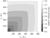 |
Fig. 1 Relative velocities, Δv (see Eq. (11)), with respect to typical stopping times, τs,1 and τs,2, of the two collision partners. |
2.2 Simulating a binary collision
To assume as little as possible about the results of a collision, we simulated it in the DEM framework, which is explained in the following.
2.2.1 Natural units
In this work we used a set of natural units that is based on Gaussian units. Notably, this means that the Coulomb force has no prefactor 1/4πε0 and, as a consequence, that the unit of time can be expressed in units of length, mass, and charge,
![Mathematical equation: $\[[\text{Time}]=\frac{\sqrt{[\text {Mass}][\text {Length}]^{3}}}{[\text {Charge}]}.\]$](/articles/aa/full_html/2025/02/aa51459-24/aa51459-24-eq22.png) (16)
(16)
Because of Eq. (16), many combinations of values whose units include at least three of the four above-mentioned ones are sufficient to construct a set of natural units. In this work specifically, we chose the particle diameter d, the particle mass m and a typical particle charge qref, which will serve as a reference charge. Thus, the corresponding natural time τ = 1 can be obtained from Eq. (16). In Table 1, the simulation parameters are listed. In order to give an idea of the orders of magnitude, plausible values in SI units are also included. We chose the particle diameter d as 0.1 mm, which is a typical size for particles used in experiments concerned with the growth and stability of agglomerates (e.g. Schwaak et al. 2024). The mass m is calculated from a particle mass density of 2500 kg/m3 (Blum et al. 1996). The reference charge of qref 106 elementary charges is of the order of magnitude of observed tribocharges (e.g. Waitukaitis et al. 2014).
2.2.2 Contact force models
A number of contact interactions are implemented in the simulation to properly resolve the agglomerate collisions. These inter-actions only produce non-zero forces and torques when particles are in contact, that is, when the particles, all having diameter d, at positions ri and rj have an overlap ξn = d – ||ri – rj|| greater than zero. All interactions are assumed to be viscoelastic: included are a normal force – the Hertz–Kuwabara–Kono (HKK) model (see Hertz 1882; Kuwabara & Kono 1987; Brilliantov et al. 1996) and tangential, rolling and torsion frictions modelled by continuous spring-dashpot sliders (C-SDSs; see Führer et al. 2024). For a detailed description of the interactions, refer to Appendix A.
Parameter values used in the simulations, given both in natural units (NU) and SI units.
2.2.3 Electrostatic interactions
All particles carry a charge of magnitude q and sign si in their centre and interact via the Coulomb force:
![Mathematical equation: $\[\boldsymbol{F}_{\mathrm{C}}=s_{i} s_{j} \frac{q^{2}}{\left\|\boldsymbol{r}_{i j}\right\|^{3}} \boldsymbol{r}_{i j}.\]$](/articles/aa/full_html/2025/02/aa51459-24/aa51459-24-eq23.png) (17)
(17)
Unfortunately, calculating all interactions between two large agglomerates is very costly, as the number of Coulomb forces grows quadratically with the number of particles; because of that, the complexity of a DEM time step for a collision with NDEM particles is ![Mathematical equation: $\[O\left(N_{\text {DEM}}^{2}\right)\]$](/articles/aa/full_html/2025/02/aa51459-24/aa51459-24-eq24.png) . Therefore, in the following, we discuss an approximation that reduces computational cost very efficiently.
. Therefore, in the following, we discuss an approximation that reduces computational cost very efficiently.
Not describing an agglomerate as a number of primary particles but as a single rigid body with a given multipole field decreases the number of interactions to that of a two-body system – independent of the actual number of involved particles. For the simulations discussed in Sect. 3, we implemented the interactions for monopoles Q, dipoles p and quadrupoles Q. The formulas for the force F and the torque J on an agglomerate with multipole moments ![Mathematical equation: $\[\\{\tilde{Q}, \tilde{p}, \tilde{\text{Q}}\}\]$](/articles/aa/full_html/2025/02/aa51459-24/aa51459-24-eq25.png) at the coordinate origin in the field of an agglomerate with multipole moments {Q, p, Q} at position r0 are the result of a tedious but straightforward combination of the approximative electric field components
at the coordinate origin in the field of an agglomerate with multipole moments {Q, p, Q} at position r0 are the result of a tedious but straightforward combination of the approximative electric field components
![Mathematical equation: $\[E_{\nu}(\boldsymbol{r})=\frac{Q r_{\nu}}{r^{3}}+3 \frac{p_{\mu} r_{\mu}}{r^{5}} r_{\nu}-\frac{p_{\nu}}{r^{3}}+\frac{5}{2} \frac{r_{\mu} Q_{\mu \kappa} r_{\kappa}}{r^{7}} r_{\nu}-\frac{Q_{\nu \mu} r_{\mu}}{r^{5}}\]$](/articles/aa/full_html/2025/02/aa51459-24/aa51459-24-eq26.png) (18)
(18)
with the approximative force
![Mathematical equation: $\[F_{\nu}=\tilde{Q} E_{\nu}\left(-\boldsymbol{r}_{0}\right)+\left.\tilde{p}_{\mu} \frac{\partial E_{\nu}}{\partial r_{\mu}}\right|_{-\boldsymbol{r}_{0}}+\left.\frac{1}{6} \tilde{Q}_{\mu \kappa} \frac{\partial^{2} E_{\nu}}{\partial r_{\mu} \partial r_{\kappa}}\right|_{-\boldsymbol{r}_{0}}\]$](/articles/aa/full_html/2025/02/aa51459-24/aa51459-24-eq27.png) (19)
(19)
or torque
![Mathematical equation: $\[J_{\nu}=\varepsilon_{\mu \kappa \nu} \tilde{p}_{\mu} E_{\kappa}\left(-\boldsymbol{r}_{0}\right)+\left.\frac{1}{3} \varepsilon_{\mu \kappa \nu} \tilde{Q}_{\mu \lambda} \frac{\partial E_{\kappa}}{\partial r_{\lambda}}\right|_{-\boldsymbol{r}_{0}},\]$](/articles/aa/full_html/2025/02/aa51459-24/aa51459-24-eq28.png) (20)
(20)
respectively. Here, Greek letters as indices denote the Cartesian coordinates {x, y, z}, and monopoles Q cannot be confused with quadrupole tensor components Qνμ because of the absence of indices. The full formulas are presented in Appendix B.
Three conditions govern the activation of the rigid-body approximation and ensure that this approximation is reasonable and efficient:
First, an agglomerate considered to be a rigid body is not allowed to come into contact with other agglomerates, as contact forces are not calculated for rigid bodies. Additionally, a description by a finite number of multipole moments is only an approximation of a charge distribution’s far field. To satisfy these points, a distance condition is implemented. It continuously checks whether a rigid agglomerate gets too close to other agglomerates, which leads to the unfreezing of the rigid agglomerate to a soft agglomerate, that is, a non-rigid object. Additionally, this condition also only allows soft agglomerates to freeze if they are sufficiently far away from all other agglomerates. The freezing-distance factor times the maximal extent of the larger of the agglomerates is the least distance between agglomerates that still allows for the rigid-body description: if two agglomerates get closer than this distance (and they are rigid), they unfreeze, and likewise, if they move further apart than this distance (and the other two conditions below are also fulfilled), they freeze. According to this definition, the critical distance is the same for freezing and unfreezing.
Second, even if an agglomerate satisfies the distance condition, it may be subject to internal movement such as vibrations or even restructuring. Simply freezing such an object might drastically change the time evolution of the system – which is why the temperature condition needs to be satisfied before a soft agglomerate may freeze. The name stems from the connection to the granular temperature of the agglomerate; however, the condition is stricter than simply demanding a small granular temperature. To calculate the internal movements, we changed into the body’s frame of reference, that is, we stripped the centre of mass motion and rotating with the agglomerate’s angular velocity. Then, the translational and rotational kinetic energies of each particle are calculated. The maximum particle energy – this is where the condition is more restrictive compared with a temperature threshold – is now monitored for a time period given by expected oscillation frequencies. Only if the maximum energy is lower than the freezing-temperature parameter for the entire time, an agglomerate is allowed to freeze.
Third, as the equations of motion as well as the multipole interactions of a rigid body are more complex than those of primary particles, it is to be expected that the benefits for freezing only outweigh the additional cost from a certain agglomerate size onwards. Therefore, the size condition only allows freezing for agglomerates that consist of at least as many particles as a chosen minimum freezing size. This sweet spot can be estimated by benchmarking the cost per time step. In contrast to the previous conditions, the size condition is purely performance related and has no further impact on the validity of the approximation.
The strictness of these conditions is controlled by three parameters: the freezing distance factor, the freezing temperature and the minimum freezing size. For the simulation results presented in this work, we chose a freezing distance factor and minimum freezing size of 3 and a freezing temperature of 10−3md2/τ2. We checked on one of the datasets presented below that the parameters above yield the same results as a simulation with the rigid-body approximation turned off.
In addition to the performance increase through the reduction in the number of interactions, describing agglomerates as rigid bodies has another benefit. As the time step size is limited by the necessary resolution of particle collisions, as discussed in the next section, eliminating some or even all soft agglomerates may allow for larger time step sizes.
2.2.4 Time integration and step size
We used the midpoint method to integrate the DEM time evolution: First, we approximated all dynamical variables ui(t) at time t + Δt/2 as
![Mathematical equation: $\[u_{i}(t+\Delta t / 2)=u_{i}(t)+\frac{\Delta t}{2} \dot{u}_{i}(t).\]$](/articles/aa/full_html/2025/02/aa51459-24/aa51459-24-eq29.png) (21)
(21)
Knowing these ui(t + Δt/2), we either directly know their time derivatives ![Mathematical equation: $\[\dot{u}_{i}(t+\Delta t / 2)\]$](/articles/aa/full_html/2025/02/aa51459-24/aa51459-24-eq30.png) as well (e.g. velocities in the case of positions) or we can calculate them from the ui(t + Δt/2) (e.g. forces and accelerations from positions and velocities). Then, the midpoint method yields
as well (e.g. velocities in the case of positions) or we can calculate them from the ui(t + Δt/2) (e.g. forces and accelerations from positions and velocities). Then, the midpoint method yields
![Mathematical equation: $\[u_{i}(t+\Delta t)=u_{i}(t)+\Delta t \dot{u}_{i}(t+\Delta t / 2)\]$](/articles/aa/full_html/2025/02/aa51459-24/aa51459-24-eq31.png) (22)
(22)
for the full time step t → t + Δt.
Importantly, each collision must be simulated long enough that no significant amount of re-agglomeration is omitted. As there is no reliable way to estimate whether agglomerates will collide again in a reasonable amount of time in many-particle systems (e.g. using escape velocities), we checked that our results do not change when simulating the collisions for twice as long, after all agglomerates start to pairwise move away from each other.
For the integration, the time step size Δt must not only be small to reduce the overall error, it is also important that it is smaller than the timescale of the fastest physical process that we want to simulate. In the case of this simulation, there are two important timescales: the contact time during a collision and the oscillation frequencies of the C-SDSs.
The contact time of two (uncharged) particles for given relative velocities is well described by a power law within the HKK model (see Schwager & Pöschel 1998). Therefore, its parameters depend on the stiffness kn as well as the damping ηn and can be easily fitted from the results of a number of preliminarily simulated two-particle collisions at varying impact velocities. As the contact time decreases monotonically with increasing relative velocities, the shortest contact time is defined by the largest relative velocity between two particles that are in contact or may make contact in the next step. Given this minimum contact time τmin, the current step size is set to the smaller one of
![Mathematical equation: $\[\Delta t=\frac{\tau_{\text {min}}}{20}\]$](/articles/aa/full_html/2025/02/aa51459-24/aa51459-24-eq32.png) (23)
(23)
and the maximum allowed step size Δtmax = 10−3τ, which must be small enough to properly resolve the oscillations of the C-SDSs. They behave like damped springs when oscillating; therefore, their frequencies only depend on the respective model parameters. The simulation uses Δtmax if all agglomerates are described as rigid bodies.
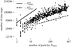 |
Fig. 2 Number of time steps for a collision simulation as a function of the total number of particles, NDEM, involved in the collision. Shown are 900 data points for collisions in the ensemble of populations with particle charge q = 1.1qref. Both axes have a logarithmic scale, and two power laws are shown for reference. |
2.3 Computational cost and complexity
The simulations presented in Sect. 3 were performed on two Intel® Xeon® Gold 6348 CPU (2.60 GHz) processors, with run times of less than two weeks per simulated population. Each population’s evolution was calculated on a single core so that a total of 56 evolutions could be simulated at once.
Roughly 95% of the CPU time is spent on performing the DEM collisions, everything else (updating collision rates, drawing new collision partners, writing outputs etc.) only makes up the remaining few percent. Not using any further approximations, the complexity of a DEM time step involving NDEM particles will be ![Mathematical equation: $\[O\left(N_{\text {DEM}}^{2}\right)\]$](/articles/aa/full_html/2025/02/aa51459-24/aa51459-24-eq33.png) for at least some time steps because of the long-range Coulomb interaction (the rigid body approximation will never be applicable during the actual contact of the agglomerates).
for at least some time steps because of the long-range Coulomb interaction (the rigid body approximation will never be applicable during the actual contact of the agglomerates).
The number of DEM time steps necessary to carry out an agglomerate collision depends on, for example, the initial distance, the relative velocity, the agglomerates’ contact time, and the finishing conditions, all of which depend on the particle number in a complicated way. Hence, we present the number of time steps for some exemplary collisions in the investigated system in Fig. 2.
The complexity of a brute force update of the collision rates discussed in Sect. 2.1.1 for NA agglomerates is ![Mathematical equation: $\[O\left(N_{\mathrm{A}}^{2}\right)\]$](/articles/aa/full_html/2025/02/aa51459-24/aa51459-24-eq34.png) , but can be reduced to O (NA) if the rates are only recalculated for collisions with agglomerates created in the most recent collision (assuming their number is of the order of one) for the system studied in this work. In general, if the environment (density, turbulence strength etc.) is not in a steady state, all collision rates have to be recalculated after each collision. The calculations of properties of an agglomerate of size M required for the rate update (maximal extent, radius of gyration etc.) have a complexity linear in M – however, as these quantities also have to be calculated in every time step of the DEM part, they are readily available and do not cost any additional time.
, but can be reduced to O (NA) if the rates are only recalculated for collisions with agglomerates created in the most recent collision (assuming their number is of the order of one) for the system studied in this work. In general, if the environment (density, turbulence strength etc.) is not in a steady state, all collision rates have to be recalculated after each collision. The calculations of properties of an agglomerate of size M required for the rate update (maximal extent, radius of gyration etc.) have a complexity linear in M – however, as these quantities also have to be calculated in every time step of the DEM part, they are readily available and do not cost any additional time.
How to estimate the number of collisions needed to simulate a given physical time? The average waiting time, which is the average time increment per collision, is given by Eq. (4). The sum in the denominator has ![Mathematical equation: $\[N_{\mathrm{A}}^{2}, N_{\mathrm{A}} \in\left(N_{\mathrm{A}, \text {init}} / 2, N\right]\]$](/articles/aa/full_html/2025/02/aa51459-24/aa51459-24-eq35.png) , terms (kept larger than NA,init/2 by the topping up algorithm), where NA,init denotes the initial number of agglomerates. This leads to a number of needed collisions of the order of
, terms (kept larger than NA,init/2 by the topping up algorithm), where NA,init denotes the initial number of agglomerates. This leads to a number of needed collisions of the order of ![Mathematical equation: $\[N_{\mathrm{A}, \text {init}}^{2}\]$](/articles/aa/full_html/2025/02/aa51459-24/aa51459-24-eq36.png) or N2 at best or worst, respectively. Moreover, the number of particles in the population N, appears in the numerator of Eq. (4), and also non-trivially affects the collision cross-sections and relative velocities in the denominator, as discussed earlier in this section. The situation is further complicated, as N and NA change in time because of the topping up algorithm, agglomeration, and fragmentation. To get a quantitative idea about how many collisions were necessary for the results in Sect. 3, see Fig. 3. As expected, we notice a correlation between the number of collisions and the number of agglomerates in the populations at the final time t = 98 years. However, the influence of the number of particles is less clear. To understand Fig. 3 in more detail, we need some results from – and, thus, delay its discussion to the end of – Sect. 3.1.
or N2 at best or worst, respectively. Moreover, the number of particles in the population N, appears in the numerator of Eq. (4), and also non-trivially affects the collision cross-sections and relative velocities in the denominator, as discussed earlier in this section. The situation is further complicated, as N and NA change in time because of the topping up algorithm, agglomeration, and fragmentation. To get a quantitative idea about how many collisions were necessary for the results in Sect. 3, see Fig. 3. As expected, we notice a correlation between the number of collisions and the number of agglomerates in the populations at the final time t = 98 years. However, the influence of the number of particles is less clear. To understand Fig. 3 in more detail, we need some results from – and, thus, delay its discussion to the end of – Sect. 3.1.
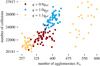 |
Fig. 3 Number of collisions simulated and number of agglomerates at the end of the evolution at t = 98 years for each of the 3 × 56 populations discussed in Sect. 3. All populations started with NA,init = 500 dimers. The colours indicate the three ensembles, which differ in terms of particle charges, q. The populations with q = 0.9qref finished with N = 2000 particles (duplicated once) and the populations with q = 1.0qref finished with N = 4000 particles (duplicated twice). Two distinct sets of populations with q = 1.1qref are visible, with (NA < 325, N = 4000) and (NA > 475, N = 8000), respectively. The populations with N = 8000 are duplicated three times. |
3 Results
In the presented simulations, the initial agglomerate population consists of neutral dimers with random orientations and no angular momenta. Each dimer is built out of two spherical particles in contact, which carry a charge of equal magnitude. Apart from their polarity, all particles are equal. We simulated an ensemble of 56 systems – differing in their (random) initial configuration – for each studied particle charge. Table 1 contains all other required parameters.
Each population started off with 1000 particles. To improve the statistics in the following analysis, we view the collection of all individual populations – which all are representative samples that evolved independently under equal conditions – as a single large population. As the macroscopic time step sizes (see Sect. 2.1.1) are stochastic in nature and interpolation is not an option for the given data, it may not be trivial to see, which individual populations are included in the combined population at a time t. Considering that we know the population exactly at the times, at which it changes (because of a collision), we also know that the population remains unchanged in the time between two collisions. Therefore, the combined population at time t consists of all those individual populations that were produced by the last collisions before the time t.
We want to point out that the term size distribution is often used for the distribution of the agglomerate masses (measured in numbers of constituent particles) and not for the distribution of, say, their radii (see e.g. Steinpilz et al. 2020). To be consistent with the afore mentioned literature, we too call the distribution of masses ASD.
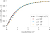 |
Fig. 4 Time evolution of the average agglomerate size for three different particle charges, collapsed onto each other to reveal the universal exponential convergence. The average sizes, ⟨M⟩(t), and average asymptotic sizes, ⟨M⟩∞, are measured in numbers of primary particles. Both the average asymptotic sizes and the characteristic times, t*, are used as fit parameters; refer to Table 2 for their values. The dashed line is included to guide the eye. |
3.1 Stationarity of the size distribution
As we simulate a driven granular gas where agglomeration and fragmentation of agglomerates can occur, the possibility of an emerging stationary ASD is a reasonable assumption. For example, Zsom et al. (2010) discussed the possibility of emerging quasi-steady states in the midplane of a disk due to bouncing, and Brilliantov et al. (2015) explained the stationarity of the grain size distribution in Saturn’s rings by assuming an agglomeration–fragmentation equilibrium. Here we should distinguish between the two trivial (and extreme) distributions – the existence of either only monomers or only one agglomerate that contains the entire mass of the population – and all other non-trivial ones. In the context of planet formation, conditions that result in the latter trivial case, that is, conditions that result in a run-away growth, are of particular interest.
To check whether the ASD reached a stationary state, it is, in principle, necessary to check if all moments of the distribution become stationary. In practice, however, this is not feasible. For the purpose of this work, we checked the evolution of the average agglomerate size (Fig. 4) and a contour plot of the entire distribution’s evolution (Fig. 5). Both figures indicate stationarity of the ASD for the two larger charges; however, the simulated time was not sufficiently long to reach the stationary state of the system with q = 0.9qref, which converges more slowly.
Greater charges result in larger agglomerates – as might be expected – visible in Fig. 5 and quantified by the asymptotic average agglomerate sizes ⟨M⟩∞ in Table 2. In addition, the time needed to reach the stationary distribution depends on the particle charge as well: the characteristic time t* of the average size’s exponential convergence to its asymptotic value gets smaller with increased charge (see Table 2).
Now that we know that the average agglomerate size, which is given by the number of particles, N (equivalent to the total mass of the population in our case) and the number of agglomerates, NA, by definition,
![Mathematical equation: $\[\langle M\rangle=\frac{N}{N_{\mathrm{A}}}\]$](/articles/aa/full_html/2025/02/aa51459-24/aa51459-24-eq37.png) (24)
(24)
converges to an asymptotic value ⟨M⟩∞ (see Fig. 4), we can understand Fig. 3 in more detail. Using our fit values for ⟨M⟩∞ (Table 2), we can calculate asymptotic values for the ensemble average of the number of agglomerates NA,∞(N). A single population of finite size will always only fluctuate around this value, and only the ensemble average will actually tend to it. For example, we get NA,∞ ≈ 272 and NA,∞ ≈ 544 for N = 4000 and N = 8000, respectively, for the populations with particle charges q = 1.1qref. This is consistent with with the data shown in Fig. 3: the populations with particle charges q = 1.1qref are split into two sets, according to their numbers of particles N = 4000, 8000. In general, our populations start off with very small agglomerates, which leads to a decreasing number of agglomerates due to agglomeration. Neglecting fluctuations, the topping up algorithm will keep duplicating the populations, until NA,∞(N) is larger than the lower bound for the number of agglomerates, NA,init/2 = 250. In the case of the q = 1.1qref-ensemble, however, the asymptotic number of agglomerates NA,∞(4000) ≈ 272 is so close to the lower bound that fluctuations have caused some populations to be duplicated, resulting in the two sets of populations visible in Fig. 3.
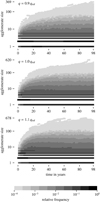 |
Fig. 5 Time evolution of the ASD for different particle charges. The agglomerate sizes are measured in numbers of primary particles, and their frequencies are normalised by the total number of agglomerates at a certain time. |
3.2 Agglomerate size distribution
As previously stated, both Steinpilz et al. (2020) and Singh & Mazza (2018) studied the ASD for charged particles – in contrast to this work, for freely cooling systems – and both reported a power law with an exponent of −1.3 to −1.4, which roughly fits with the exponent of −1.5 produced in our simulations (see Fig. 6). However, the power law describes the ASD only for small agglomerates: the tails of the distribution actually follow an exponential distribution. This is also supported by the fact that the deviation from the power law can already be seen in the results from Singh & Mazza (2018) (in their Fig. 4, the data deviate from the power-law fit for s > 10; s is their measure for the agglomerate size). We estimated the probabilities by calculating the difference quotients of the empirical cumulative distribution function for agglomerate sizes. The employed difference quotients only take into account sizes that occur at least once.
By rescaling the agglomerate sizes, we collapsed the ASDs in Fig. 6 onto each other and show that the distribution changes under the variation of the particle charge only through the characteristic size M*, which we used as a fit parameter (see Table 2). Notably, this characteristic size M* is larger than the average size ⟨M⟩(t = 98 yrs) in Fig. 4. This is because small agglomerates (the part that fits the power-law description) are more frequent than a pure exponential distribution would suggest. Therefore, the average is skewed towards smaller agglomerates, whereas the exponential decay in the tails is not affected.
4 Conclusion
In this paper we have presented a novel hybrid method for simulations of ASD evolutions, combining the efficiency of probability-based simulations and the precision of DEM simulations for the microscopic processes of agglomerate collisions. We find that the average agglomerate size converges exponentially fast to a charge-dependent asymptotic size, where the increased stability of higher charges allows for further agglomeration. Furthermore, an analysis of the full ASD reveals that the system reaches a steady state on a timescale of 100 years for our parameter choices.
The observed exponential tails of the ASD are seemingly in contradiction with the power laws presented by Steinpilz et al. (2020) and Singh & Mazza (2018). However, the present simulation was able to produce better statistics for agglomerates of far larger particle numbers, which allowed us to study the tail behaviour in much more detail. Our findings are supported by the visible deviation from the Singh & Mazza (2018) power law shown in their Fig. 4, panels b–d. From these results alone, it is not possible to make any quantitative claims about size distributions in protoplanetary disks; more extensive parameter studies are needed. However, the presence of an exponential drop-off in the steady state might be an indication of the existence of a growth barrier, beyond which agglomerate sizes are not impossible but extremely unlikely.
We want to point out that it generally is straightforward to extend the presented model to include additional physical processes. As long as the main assumptions – a sufficiently dilute granular gas and collision times much shorter than particleenvironment coupling times – are satisfied, the effects of different driving mechanisms (e.g. radial drift or sedimentation) and spatial inhomogeneities of the agglomerate number density, just to name a few, solely affect the relative velocities and collision rates. Therefore, a slight modification of the code allows for the study of those processes’ roles in a plethora of systems.
While in this paper we have focused on the role of the particle charges, studying local variations in turbulence strength might be crucial in understanding the local disk structure with regard to the ASD. Furthermore, an investigation of the robustness of the qualitative behaviour and the shape of the ASD under different driving mechanisms would be an important continuation of this study. Also, it is possible to classify collisions according to their outcomes (e.g. the types proposed by Zsom et al. (2010), their Sect. 3.4.) and use these statistics to evaluate their relevance with respect to agglomerate growth and growth barriers. Additionally, as the results of our hybrid method encompass not just agglomerate sizes but also the actual positions of the constituent particles, we intend to analyse these collisionally grown agglomerates with respect to porosities and binding energies for charged as well as adhesive particles (long-range vs short-range interactions) in the future.
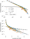 |
Fig. 6 ASDs for three different charges at t = 98 years. All agglomerate sizes, M, are rescaled with characteristic sizes, M* (see Table 2), such that the tails have a slope of −1 in the semi-logarithmic (lower) plot. The exponential function and power law are included to guide the eye. The upper and lower plots show the same data but with logarithmically and linearly scaled abscissae, respectively. |
Acknowledgements
We thank the anonymous referee for thoroughly examining our manuscript and for suggesting many changes that strengthened the message of this paper. The presented research is funded by the Deutsche Forschungsgemeinschaft (DFG, German Research Foundation) – Projektnummer(458889524). We acknowledge support by the Open Access Publication Fund of the University of Duisburg-Essen.
Appendix A Details of implemented contact forces
All contact forces have in common that they only act on particles that are in direct contact, that is, with a particle radius R and particle positions ri and rj, the overlap ξn = 2R – ||ri – rj|| must be greater than zero. For this study, all particles are of the same size, 2R, and mass, m.
We note that we did not implement any cohesive forces. This is because, as already mentioned by, for example, Steinpilz et al. (2020), the cohesion between micrometre-sized particles is way too small to have any significant influence on the stability of agglomerates when collision velocities exceed cm/s. Therefore, the cohesion would always be negligible compared with the Coulomb forces presented in Sect. 2.2.3.
We denote the spring stiffness and damping parameters as well as friction coefficients as k, γ and μ, respectively. We add an index to these parameters, indicating to which type of contact force they belong (see Table 1): n (normal), t (tangential), s (torsion or spin), and r (rolling). We chose all parameters such that the contact is critically damped, and the resulting time steps yield reasonable computational efforts.
A.1 Normal force
The normal force presented in the following is denoted as the force acting on the particle i; thus, the normal vector is
![Mathematical equation: $\[\boldsymbol{n}=\frac{\boldsymbol{r}_{i}-\boldsymbol{r}_{j}}{\left\|\boldsymbol{r}_{i}-\boldsymbol{r}_{j}\right\|}.\]$](/articles/aa/full_html/2025/02/aa51459-24/aa51459-24-eq38.png) (A.1)
(A.1)
Furthermore, we used the effective radius
![Mathematical equation: $\[R_{\text {eff }}=\frac{R R}{R+R}=\frac{R}{2}\]$](/articles/aa/full_html/2025/02/aa51459-24/aa51459-24-eq39.png) (A.2)
(A.2)
and the analogously defined effective mass
![Mathematical equation: $\[m_{\text {eff }}=\frac{m}{2}.\]$](/articles/aa/full_html/2025/02/aa51459-24/aa51459-24-eq40.png) (A.3)
(A.3)
The relative velocity vij = vi – vj has the normal component
![Mathematical equation: $\[\boldsymbol{v}_{\mathrm{n}}=v_{\mathrm{n}} \boldsymbol{n}=\left(\boldsymbol{n} \cdot \boldsymbol{v}_{i j}\right) \boldsymbol{n}.\]$](/articles/aa/full_html/2025/02/aa51459-24/aa51459-24-eq41.png) (A.4)
(A.4)
For the normal contact force Fn, we implemented the HKK model (Hertz 1882; Kuwabara & Kono 1987; Brilliantov et al. 1996): The repulsion term (Hertz) and the damping term (Kuwabara–Kono) are combined into the total normal contact force
![Mathematical equation: $\[F_{\mathrm{n}}=\sqrt{R_{\mathrm{eff}}} k_{\mathrm{n}} \xi_{\mathrm{n}}^{3 / 2}-m_{\mathrm{eff}} \sqrt{R_{\mathrm{eff}} \xi_{\mathrm{n}}} \gamma_{\mathrm{n}} v_{\mathrm{n}}.\]$](/articles/aa/full_html/2025/02/aa51459-24/aa51459-24-eq42.png) (A.5)
(A.5)
A.2 Tangential forces and torques
All implemented tangential forces and torques include sticking and sliding, implemented via the continuous spring-dashpot slider (Führer et al. 2024), which is a modification of the discrete spring-dashpot slider as presented by Luding (2008). Apart from the corrected spring-displacement update, the forces, torques, and relative velocities are implemented analogously to in Luding (2008). In essence, all forces and torques are calculated from the limited reaction force of a deforming viscoelastic material,
![Mathematical equation: $\[\boldsymbol{F}_{\mathrm{SDS}}=\min \left(-k \boldsymbol{\xi}-\gamma \boldsymbol{v}, \mu F_{\mathrm{n}}\right),\]$](/articles/aa/full_html/2025/02/aa51459-24/aa51459-24-eq43.png) (A.6)
(A.6)
where ξ denotes the spring displacement, modelling the material deformation, and v the respective relative velocity, not considering material deformation (for details, see Führer et al. 2024).
We note that the parameters k, γ, and μ differ in their units for the different modes; only tangential and rolling interactions share the same units. This is because Hertz’s contact model is based on the contact area and not a linear displacement, and the torsion mode is concerned with angular (not length) changes.
Appendix B Multipole interaction formulas
The full formulas for the second order multipole–multipole interactions, calculated from Eqs. (18), (19) and (20) — using
![Mathematical equation: $\[A=Q_{v \mu} \tilde{Q}_{v \mu},\]$](/articles/aa/full_html/2025/02/aa51459-24/aa51459-24-eq44.png) (B.1)
(B.1)
![Mathematical equation: $\[(\boldsymbol{B})_{\kappa}=\varepsilon_{\nu \mu \kappa} \tilde{Q}_{\nu \mu},\]$](/articles/aa/full_html/2025/02/aa51459-24/aa51459-24-eq45.png) (B.2)
(B.2)
![Mathematical equation: $\[(\boldsymbol{C})_{\kappa}=\varepsilon_{\nu \mu \kappa} \tilde{Q}_{\nu \lambda} Q_{\lambda \mu},\]$](/articles/aa/full_html/2025/02/aa51459-24/aa51459-24-eq46.png) (B.3)
(B.3)
and the identity matrix I — are
![Mathematical equation: $\[\begin{aligned}& \boldsymbol{F}=\frac{\tilde{Q}}{r^3}\left(Q \boldsymbol{r}+3 \frac{\boldsymbol{p} \cdot \boldsymbol{r}}{r^2} \boldsymbol{r}-\boldsymbol{p}+\frac{5}{2} \frac{\boldsymbol{r} \cdot \mathrm{Q} \boldsymbol{r}}{r^4} \boldsymbol{r}-\frac{\mathrm{Q} \boldsymbol{r}}{r^2}\right) \\& +\frac{Q}{r^3}\left(1-3 \frac{\boldsymbol{r} \otimes \boldsymbol{r}}{r^2}\right) \tilde{\boldsymbol{p}}+3 \frac{1}{r^5}\left(\boldsymbol{p} \cdot \tilde{\boldsymbol{p}} \boldsymbol{r}+\boldsymbol{p} \cdot \boldsymbol{r} \tilde{\boldsymbol{p}}-5 \frac{\boldsymbol{p} \cdot \boldsymbol{r} \tilde{\boldsymbol{p}} \cdot \boldsymbol{r} \boldsymbol{r}}{r^2}\right) \\& +3 \frac{\tilde{p} \cdot \boldsymbol{r}}{r^5} \boldsymbol{p}+5 \frac{\boldsymbol{r}}{r^7} \cdot\left(\mathrm{Q} \tilde{\boldsymbol{p}} \boldsymbol{r}+\frac{1}{2} \mathrm{Q} r \tilde{p}-\frac{7}{2} \frac{\tilde{p} \cdot \boldsymbol{r}}{r^2} \mathrm{Q} \boldsymbol{r} \boldsymbol{r}\right) \\& -\left(\mathrm{Q} \tilde{p}-5 \frac{r \cdot \tilde{p} \mathrm{Q} \boldsymbol{r}}{r^2}\right) \frac{1}{r^5}+\frac{3}{6} \frac{Q}{r^5}\left(-2 \tilde{\mathrm{Q}} \boldsymbol{r}+5 \boldsymbol{r} \frac{\boldsymbol{r} \cdot \tilde{\mathrm{Q}} \boldsymbol{r}}{r^2}\right) \\& +\frac{3}{2 r^5}\left(2 \tilde{\mathrm{Q}} \boldsymbol{p}-10 \frac{\boldsymbol{p} \cdot \tilde{\mathrm{Q}} r}{r^2} \boldsymbol{R}+\boldsymbol{p} \cdot \boldsymbol{r}\left(-10 \frac{\tilde{\mathrm{Q}} \boldsymbol{r}}{r^2}+35 \frac{\boldsymbol{R} \cdot \tilde{\mathrm{Q}} r}{r^4} r\right)\right. \\& \left.-5 \frac{r \cdot \tilde{\mathrm{Q}} \boldsymbol{r}}{r^2} \boldsymbol{p}\right)+\frac{5}{6 r^7}\left(A r+2 \tilde{\mathrm{Q}}\mathrm{Q} r-14 \frac{r \cdot \mathrm{Q} \mathrm{Q} r}{r^2} \boldsymbol{r}\right. \\& \left.+\frac{7}{2} r \cdot \mathrm{Q} r\left(-2 \frac{\tilde{\mathrm{Q}} r}{r^2}+9 \frac{r \cdot \tilde{\mathrm{Q}} r}{r^4} r\right)+2 \mathrm{Q} \tilde{\mathrm{Q}} r-7 \frac{r \cdot \tilde{\mathrm{Q}} r}{r^2} \mathrm{Q} r\right)\end{aligned}\]$](/articles/aa/full_html/2025/02/aa51459-24/aa51459-24-eq47.png)
and
![Mathematical equation: $\[\begin{aligned}\boldsymbol{J}= & \frac{\tilde{\boldsymbol{p}} \times \boldsymbol{r}}{r^3}\left(Q+3 \frac{\boldsymbol{p} \cdot \boldsymbol{r}}{r^2}+\frac{5}{2} \frac{\boldsymbol{r} \cdot \mathrm{Q} \boldsymbol{r}}{r^4}\right)-\frac{\tilde{\boldsymbol{p}} \times \boldsymbol{p}}{r^3}-\frac{\tilde{\boldsymbol{p}} \times(\mathrm{Q} \boldsymbol{r})}{r^5} \\& +\frac{Q}{3 r^3}\left(\boldsymbol{B}-3 \frac{(\tilde{\mathrm{Q}} \boldsymbol{r}) \times \boldsymbol{r}}{r^2}\right)+\frac{1}{r^5}((\tilde{\mathrm{Q}} \boldsymbol{p}) \times \boldsymbol{r}+(\tilde{\mathrm{Q}} \boldsymbol{r}) \times \boldsymbol{p} \\& \left.+\boldsymbol{p} \cdot \boldsymbol{r}\left(\boldsymbol{B}-5 \frac{(\tilde{\mathrm{Q}} \boldsymbol{r}) \times \boldsymbol{r}}{r^2}\right)\right)+\frac{5}{3 r^7}\left((\tilde{\mathrm{Q Q}} \boldsymbol{r}) \times \boldsymbol{r}+\frac{1}{2} \boldsymbol{r} \cdot \mathrm{Q} \boldsymbol{r}(\boldsymbol{B}\right. \\& \left.\left.-7 \frac{(\tilde{\mathrm{Q}} \boldsymbol{r}) \times \boldsymbol{r}}{r^2}\right)+(\tilde{\mathrm{Q}} \boldsymbol{r}) \times(\mathrm{Q} \boldsymbol{r})\right)-\frac{\boldsymbol{C}}{r^5},\end{aligned}\]$](/articles/aa/full_html/2025/02/aa51459-24/aa51459-24-eq48.png)
evaluated at r = −r0.
References
- Birnstiel, T., Dullemond, C. P., & Brauer, F. 2010, A&A, 513, A79 [NASA ADS] [CrossRef] [EDP Sciences] [Google Scholar]
- Birnstiel, T., Ormel, C. W., & Dullemond, C. P. 2011, A&A, 525, A11 [NASA ADS] [CrossRef] [EDP Sciences] [Google Scholar]
- Birnstiel, T., Fang, M., & Johansen, A. 2016, Space Sci. Rev., 205, 41 [Google Scholar]
- Blum, J., & Wurm, G. 2008, ARA&A, 46, 21 [Google Scholar]
- Blum, J., Wurm, G., Kempf, S., & Henning, T. 1996, Icarus, 124, 441 [NASA ADS] [CrossRef] [Google Scholar]
- Brilliantov, N. V., Spahn, F., Hertzsch, J.-M., & Pöschel, T. 1996, Phys. Rev. E, 53, 5382 [NASA ADS] [CrossRef] [Google Scholar]
- Brilliantov, N., Krapivsky, P. L., Bodrova, A., et al. 2015, PNAS, 112, 9536 [NASA ADS] [CrossRef] [Google Scholar]
- Demirci, T., Teiser, J., Steinpilz, T., et al. 2017, ApJ, 846, 48 [Google Scholar]
- Dominik, C., & Tielens, A. G. G. M. 1997, ApJ, 480, 647 [Google Scholar]
- Draine, B. T., Dale, D. A., Bendo, G., et al. 2007, ApJ, 663, 866 [NASA ADS] [CrossRef] [Google Scholar]
- Estrada, P. R., Cuzzi, J. N., & Morgan, D. A. 2016, ApJ, 818, 200 [NASA ADS] [CrossRef] [Google Scholar]
- Führer, F., Brendel, L., & Wolf, D. E. 2024, Granular Matter, 26, 53 [CrossRef] [Google Scholar]
- Güttler, C., Blum, J., Zsom, A., Ormel, C. W., & Dullemond, C. P. 2010, A&A, 513, A56 [Google Scholar]
- Hertz, H. 1882, Journal für die reine und angewandte Mathematik, 1882, 156 [CrossRef] [Google Scholar]
- Ivlev, A. V., Morfill, G. E., & Konopka, U. 2002, Phys. Rev. Lett., 89, 195502 [CrossRef] [Google Scholar]
- Jansen, A. P. J. 2012, An Introduction to Kinetic Monte Carlo Simulations of Surface Reactions (Berlin, Heidelberg: Springer) [CrossRef] [Google Scholar]
- Johansen, A., Brauer, F., Dullemond, C., Klahr, H., & Henning, T. 2008, A&A, 486, 597 [NASA ADS] [CrossRef] [EDP Sciences] [Google Scholar]
- Kelling, T., Wurm, G., & Köster, M. 2014, ApJ, 783, 111 [Google Scholar]
- Kuwabara, G., & Kono, K. 1987, Jpn. J. Appl. Phys., 26, 1230 [NASA ADS] [CrossRef] [Google Scholar]
- Liffman, K. 1992, J. Comput. Phys., 100, 116 [NASA ADS] [CrossRef] [Google Scholar]
- Luding, S. 2008, Granular Matter, 10, 235 [CrossRef] [Google Scholar]
- Nakagawa, Y., Sekiya, M., & Hayashi, C. 1986, Icarus, 67, 375 [Google Scholar]
- Okuzumi, S., Tanaka, H., Takeuchi, T., & Sakagami, M.-a. 2011, ApJ, 731, 95 [Google Scholar]
- Ormel, C. W., & Cuzzi, J. N. 2007, A&A, 466, 413 [NASA ADS] [CrossRef] [EDP Sciences] [Google Scholar]
- Ormel, C. W., Spaans, M., & Tielens, A. G. G. M. 2007, A&A, 461, 215 [NASA ADS] [CrossRef] [EDP Sciences] [Google Scholar]
- Pinilla, P., Birnstiel, T., Ricci, L., et al. 2012, A&A, 538, A114 [NASA ADS] [CrossRef] [EDP Sciences] [Google Scholar]
- Ruan, X., & Li, S. 2022, Phys. Rev. E, 106, 034905 [CrossRef] [Google Scholar]
- Scheffler, T., & Wolf, D. E. 2002, Granular Matter, 4, 103 [CrossRef] [Google Scholar]
- Schwaak, J., Führer, F., Wolf, D. E., et al. 2024, A&A, 691, A127 [NASA ADS] [CrossRef] [EDP Sciences] [Google Scholar]
- Schwager, T., & Pöschel, T. 1998, Phys. Rev. E, 57, 650 [CrossRef] [Google Scholar]
- Simon, J. B., Armitage, P. J., Li, R., & Youdin, A. N. 2016, ApJ, 822, 55 [Google Scholar]
- Singh, C., & Mazza, M. G. 2018, Phys. Rev. E, 97, 022904 [NASA ADS] [CrossRef] [Google Scholar]
- Smith, M., & Matsoukas, T. 1998, Chem. Eng. Sci., 53, 1777 [Google Scholar]
- Squire, J., & Hopkins, P. F. 2018, MNRAS, 477, 5011 [Google Scholar]
- Steinpilz, T., Joeris, K., Jungmann, F., et al. 2020, Nat. Phys., 16, 225 [Google Scholar]
- Tanaka, H., Wada, K., Suyama, T., & Okuzumi, S. 2012, Prog. Theor. Phys. Suppl., 195, 101 [CrossRef] [Google Scholar]
- Völk, H. J., Jones, F. C., Morfill, G. E., & Röser, S. 1980, A&A, 85, 316 [Google Scholar]
- Waitukaitis, S. R., Lee, V., Pierson, J. M., Forman, S. L., & Jaeger, H. M. 2014, Phys. Rev. Lett., 112, 218001 [Google Scholar]
- Weidenschilling, S. J. 1977, MNRAS, 180, 57 [Google Scholar]
- Weidenschilling, S. J., & Cuzzi, J. N. 1993, Protostars and Planets III (Tucson: University of Arizona Press), 1031 [Google Scholar]
- Weidling, R., Güttler, C., Blum, J., & Brauer, F. 2009, ApJ, 696, 2036 [NASA ADS] [CrossRef] [Google Scholar]
- Youdin, A. N., & Goodman, J. 2005, ApJ, 620, 459 [Google Scholar]
- Young, W. M., & Elcock, E. W. 1966, Proc. Phys. Soc., 89, 735 [CrossRef] [Google Scholar]
- Zsom, A., Ormel, C. W., Güttler, C., Blum, J., & Dullemond, C. P. 2010, A&A, 513, A57 [NASA ADS] [CrossRef] [EDP Sciences] [Google Scholar]
All Tables
Parameter values used in the simulations, given both in natural units (NU) and SI units.
All Figures
|
Fig. 1 Relative velocities, Δv (see Eq. (11)), with respect to typical stopping times, τs,1 and τs,2, of the two collision partners. |
| In the text | |
|
Fig. 2 Number of time steps for a collision simulation as a function of the total number of particles, NDEM, involved in the collision. Shown are 900 data points for collisions in the ensemble of populations with particle charge q = 1.1qref. Both axes have a logarithmic scale, and two power laws are shown for reference. |
| In the text | |
|
Fig. 3 Number of collisions simulated and number of agglomerates at the end of the evolution at t = 98 years for each of the 3 × 56 populations discussed in Sect. 3. All populations started with NA,init = 500 dimers. The colours indicate the three ensembles, which differ in terms of particle charges, q. The populations with q = 0.9qref finished with N = 2000 particles (duplicated once) and the populations with q = 1.0qref finished with N = 4000 particles (duplicated twice). Two distinct sets of populations with q = 1.1qref are visible, with (NA < 325, N = 4000) and (NA > 475, N = 8000), respectively. The populations with N = 8000 are duplicated three times. |
| In the text | |
|
Fig. 4 Time evolution of the average agglomerate size for three different particle charges, collapsed onto each other to reveal the universal exponential convergence. The average sizes, ⟨M⟩(t), and average asymptotic sizes, ⟨M⟩∞, are measured in numbers of primary particles. Both the average asymptotic sizes and the characteristic times, t*, are used as fit parameters; refer to Table 2 for their values. The dashed line is included to guide the eye. |
| In the text | |
|
Fig. 5 Time evolution of the ASD for different particle charges. The agglomerate sizes are measured in numbers of primary particles, and their frequencies are normalised by the total number of agglomerates at a certain time. |
| In the text | |
|
Fig. 6 ASDs for three different charges at t = 98 years. All agglomerate sizes, M, are rescaled with characteristic sizes, M* (see Table 2), such that the tails have a slope of −1 in the semi-logarithmic (lower) plot. The exponential function and power law are included to guide the eye. The upper and lower plots show the same data but with logarithmically and linearly scaled abscissae, respectively. |
| In the text | |
Current usage metrics show cumulative count of Article Views (full-text article views including HTML views, PDF and ePub downloads, according to the available data) and Abstracts Views on Vision4Press platform.
Data correspond to usage on the plateform after 2015. The current usage metrics is available 48-96 hours after online publication and is updated daily on week days.
Initial download of the metrics may take a while.