| Issue |
A&A
Volume 694, February 2025
|
|
|---|---|---|
| Article Number | A288 | |
| Number of page(s) | 9 | |
| Section | Planets, planetary systems, and small bodies | |
| DOI | https://doi.org/10.1051/0004-6361/202451115 | |
| Published online | 20 February 2025 | |
Enceladus and Jupiter as exoplanets: The opposition surge effect
1
Center for Space and Habitability, University of Bern,
Gesellschaftsstrasse 6,
3012
Bern,
Switzerland
2
Space Telescope Science Institute,
3700 San Martin Dr,
Baltimore,
MD
21218,
USA
3
Ludwig Maximilian University, University Observatory Munich,
Scheinerstrasse 1,
Munich
81679,
Germany
4
University of Warwick, Department of Physics, Astronomy & Astrophysics Group,
Coventry
CV4 7AL,
UK
5
University of Bern, ARTORG Center for Biomedical Engineering Research,
Murtenstrasse 50,
3008,
Bern,
Switzerland
★ Corresponding author; This email address is being protected from spambots. You need JavaScript enabled to view it.
Received:
14
June
2024
Accepted:
22
January
2024
Abstract
Planets and moons in our Solar System have strongly peaked reflected light phase curves at opposition. In this work, we produce a modified reflected light phase curve model and use it to fit the Cassini phase curves of Jupiter and Enceladus. This ‘opposition effect’ is caused by shadow hiding (SH; particles or rough terrain cast shadows which are not seen at zero phase) and coherent backscattering (CB; incoming light constructively interferes with outgoing light). We find tentative evidence for CB preference in Jupiter compared to SH, and no evidence of preference in Enceladus. We show that the full-width half-maximum (FWHM) of Jupiter’s opposition peak is an order of magnitude larger than that of Enceladus and conclude that this could be used as a solid-surface indicator for exoplanets. We investigate this and show that modelling the opposition peak FWHM in solid-surface exoplanets would be unfeasible with JWST or the Future Habitable Worlds Observatory due to the very large signal-to-noise required over a small phase range.
Key words: scattering / atmospheric effects / planets and satellites: atmospheres / planets and satellites: fundamental parameters / planets and satellites: surfaces
© The Authors 2025
 Open Access article, published by EDP Sciences, under the terms of the Creative Commons Attribution License (https://creativecommons.org/licenses/by/4.0), which permits unrestricted use, distribution, and reproduction in any medium, provided the original work is properly cited.
This article is published in open access under the Subscribe to Open model. This email address is being protected from spambots. You need JavaScript enabled to view it. to support open access publication.
1 Introduction
For over a century, observations have shown that phase curves of many Solar System bodies have sharp peaks in reflectance at opposition. It has also been shown that the moons and rocky planets produce narrower peaks than the gas giants (see, e.g. Sudarsky et al. 2005; Dyudina et al. 2016).
Two underlying mechanisms driving the ‘opposition effect’ are: shadow hiding (SH) and coherent backscattering (CB). Shadow hiding, first theorised in von Seeliger (1887), occurs on rough surfaces, for example, a rocky planet or moon. When illuminated near quadrature, the roughness casts shadows, reducing the illuminated area and the total reflected light. Close to zero phase, the particles or rough terrain hide their own shadow and the body gets much brighter when viewed face-on. As this involves the shadows cast by the incoming light, this effect only works with singly-scattered light. The second mechanism is coherent backscattering. This is an effect that works with both singly and multiply scattered light. As described thoroughly in Hapke (2002), CB occurs when the light is scattered in such a way that it coherently interferes with the incoming light and therefore the observer views an increase in brightness near zero phase. This effect can only occur in an inhomogeneous particulate medium where the particles have very high single-scattering albedos (ratio of scattering to absorption) and the particles have radii similar to the wavelength of the incoming light (Helfenstein et al. 1997).
For exoplanets, observing a phase curve is a crucial tool in characterising a planetary atmosphere. With new space and ground-based telescopes coming online, we can begin to probe smaller, more Earth-like planets. These cooler planets require us to observe in the optical to obtain a reflected-light phase curve. Due to all the possible signals which contribute to the overall phase curve, modelling these observations can be difficult and significant inhomogeneities can be detected (see, e.g. Morris et al. 2024). Therefore understanding the signals within phase curves and being able to model them correctly is crucial for the investigations of planetary atmospheres and origins.
In this paper we investigate whether the opposition effect could be detectable in exoplanet phase curves and what this would reveal about the surface and/or the atmosphere of the planet. In Section 2.2, we develop our own opposition effect phase curve model and test it with multi-wavelength phase curves of Jupiter and Enceladus (see Section 3). In Section 3.3, we investigate the differences between the full-width halfmaximum of the opposition peak in Jupiter and Enceladus. In Section 4.1 we look at whether this feature could be used as a solid-surface exoplanet detector. We detail the caveats and further interpretations in Section 5.
2 Methods
2.1 Jupiter and Enceladus Cassini data
We use multi-wavelength phase curves of both Jupiter and Enceladus previously published by Li et al. (2018) and Li et al. (2023), which reported images and combined reflectance phase curves taken with Cassini/ISS, Cassini/VIMS, and the Hubble Space Telescope (HST). Figure 1 shows these Jupiter phase curves as a function of wavelength. Due to the limited number of images taken by the Cassini flyby, the phase coverage is not homogeneous. We limit the dataset to Jupiter phase curves with sufficient phase coverage by removing phase curves with fewer than 40 dat- apoints. Figure 2 shows the Enceladus phase curves. By eye it is possible to detect, particularly for Enceladus, the sharp increase in the reflected light flux near zero phase.
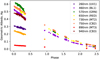 |
Fig. 1 Jupiter Cassini phase curves from Li et al. (2018), with their corresponding colour filter used in this analysis. The datapoint colours are a crude guide for the different wavelengths of the filters. |
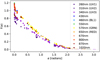 |
Fig. 2 Enceladus Cassini phase curves from Li et al. (2023), with their corresponding colour filter used in this analysis. The datapoint colours are a crude guide for the different wavelengths of the filters. Some of the filters do not have alternative names. |
2.2 Reflected light phase curve model
To fit these phase curves, we use the reflected light phase curve model developed in Heng et al. (2021), and recently applied to more planets in Morris et al. (2024). This is a unique model that can produce closed-form phase curve solutions for any scattering phase function specified by the user, making it flexible enough for both exoplanets and Solar System objects. The model is analytic and has few free parameters, allowing for fast computing time during model-fitting within a Bayesian inference framework.
Following Heng & Li (2021), we model reflected light phase curves with a single Henyey-Greenstein scattering phase function:
 (1)
(1)
where ɡ is the scattering asymmetry parameter, and α is the orbital phase angle. This phase function allows for both forward and backward scattering in variable amounts and limits the number of free parameters in the model.
The reflected light phase curve model describes the reflected flux as a function of phase F (α). We introduce an opposition peak following Hapke (2002) by multiplying an additional term (1 + δopp) so the reflected flux is:
 (2)
(2)
where F⋆ is the stellar flux, Ag is the geometric albedo, Ψ is the integral phase function and δopp(α) depends on the mechanism for the opposition surge.
There are two possible origins for the opposition peak: shadow hiding (SH) and coherent backscattering (CB). Hapke (2002) notes that the correction term associated with SH should act only on singly scattered light, whereas CB acts on both singly and multiply scattering light (caveat: high levels of multiply scattered light can dilute shadows, which can break down this assumption.) However, Hapke (2002) also notes the similarity of the SH and CB formulae and recommends that the entire opposition effect be modelled by the SH formula alone. For this reason, we apply the correction term to both singly and multiply scattered light for both SH and CB. We aim to investigate the differences between these two models at an appropriate level of accuracy as set by the precision of the data themselves.
From the empirical descriptions of Hapke (1986) and Hapke et al. (1993) we take the SH functional form to be
 (3)
(3)
where α is the phase angle, B0 is a constant describing the amplitude of the SH peak and hSH is a dimensionless constant describing the width of the SH peak. It follows that the full-width half-maximum (FWHM) of the shadow hiding peak is
 (4)
(4)
The form for CB is similar to and derives from Akkermans et al. (1988) with a random walk of photons in a scattering medium, and Hapke (2002):
 (5)
(5)
where
 (6)
(6)
We expect that SH and CB act on the phase curve together, but it is still uncertain how both effects act simultaneously. For decades, the underlying mechanism of the opposition effect on the Moon was thought to be solely shadow-hiding (see, e.g. Hapke 1963; Gehrels et al. 1964). However, by measuring the polarisation of light reflected off lunar soil samples, Hapke et al. (1993) showed that CB was also a major contributor to this effect (with later support in Helfenstein et al. 1997; Hapke et al. 1998). Therefore, whilst there is evidence for both mechanisms causing the peak in rocky bodies, it is still not understood which dominates or whether they are also both present to cause the opposition peaks seen in Jupiter and Saturn.
In this paper, we perform a comprehensive model comparison between the SH model, CB model and a non-opposition phase curve model for both Jupiter and Enceladus. We compare models with leave-one-out (LOO) cross validation statistic (Vehtari et al. 2015) and interpret our results in Section 3.1. To perform the model fitting for the phase curves, we use numpyro (Phan et al. 2019; Bingham et al. 2019) with an MCMC sampler running with 8 chains, 2000 burn-in steps and 3000 steps. We confirmed the chains had converged after the fitting procedure by inspecting the Gelman-Rubin statistic  for each free parameter (Gelman & Rubin 1992). Tables 3 and 4 shows the priors used for the free parameters within the SH model, which is the same as the priors we used for the CB model. We then measure and compare the FWHM of the opposition peaks in the Jupiter and Enceladus phase curves (see Section 3.3).
Jupiter phase curves’ preferred models.
3 Solar System results
3.1 Cross-validation favours models with opposition peaks
We fit the Jupiter phase curves with an SH model, a CB model and without any opposition model, and compare models with cross validation. The non-opposition effect model was immediately ruled out with no LOO model weight compared to the models with the opposition effect included. Therefore Jupiter likely has an opposition peak, in agreement with previous works including Heng & Li (2021), Dyudina et al. (2016) and Mayorga et al. (2016). Figure 3 shows an example of the models fitted to the 463 nm phase curve. Even by visual inspection, it is clear that the model without an opposition peak does not accurately capture the phase curve flux less than around 20 degrees.
Fitting separate CB and SH models to Jupiter’s phase curves, we found that 7 out of 8 phase curves prefer the CB model. If this is implying that CB dominates the opposition peak of Jupiter, this could be due to the lack of a surface on Jupiter, preventing dark shadows from forming (and consequently disappearing at opposition). The presence of CB implies multiple-scattering is occurring in Jupiter’s atmosphere and that the scattering particles have an inhomogeneous size distribution (Hapke 2002; Hapke et al. 1998).
We show the values of the model weights as a function of wavelength in Figure 4 and in Table 1. We do not find a trend in wavelength.
Figure 5 shows one of the Enceladus phase curves (observed with the 798 nm filter), along with the best fits for the CB, SH, and no opposition peak models. We find that the models with an opposition peak were a much better fit for all phase curves.
Seven out of 12 Enceladus phase curves prefer CB, and the other five prefer SH (see Figure 6 and Table 2). Examining the top panel of Figure 6, we see no correlation with model selection and wavelength. The non-preference of either model here could suggest that the data does have sufficient precision to distinguish between them. It also does not rule out the possibility that both effects are present on Enceladus and the opposition peak that we observe is a complex combination of the two. For example, Dlugach & Mishchenko (2013) showed that CB can take place in closely packed mediums and planetary surfaces and, as mentioned previously, we also have evidence for both SH and CB on the Moon.
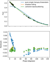 |
Fig. 3 Best fit models to one of Jupiter’s phase curves (filter BL1, 463 nm) for three different models: a pure single Henyey-Greenstein model with no additional opposition peak, shadow hiding model, and coherent backscattering model. Top panel shows the three fits and the second panel shows the residuals of these best fits. It is clear that the model with no opposition peak is the worst fit to the data. The other two models produce, by eye, almost identical fits, which is expected since the functional forms are similar. However the residuals still show subtle differences. Using the LOO model selection statistic, we conclude that the coherent backscattering model is the best fitting model for this phase curve, along with all-but-one of the other Jupiter Cassini phase curves. The corner plot showing the posteriors for the shadow hiding model in this plot are in Appendix A, Figure A.1. |
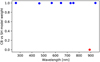 |
Fig. 4 LOO model weight of the CB model vs. the SH model for the Jupiter phase curves plotted against wavelength. When the model weight is close to 1, then the CB model is preferred (blue points), however close to 0 indicates that SH is preferred (red points). The red point shows the only phase curve where the SH model is preferred. |
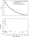 |
Fig. 5 Best fit models to one of one of Enceladus’ phase curves (filter 798 nm) for three different models: a pure single Henyey-Greenstein model with no additional opposition peak, shadow hiding model, and coherent backscattering model. Top panel shows the fits and the second panel shows the residuals of these best fits. It is clear that the model with no opposition peak is the worst fit to the data. The other two models produce, by eye, almost identical fits, which is expected since the functional forms are similar. However the residuals still show subtle differences. Using the LOO model selection statistic allows us to conclude that the coherent backscattering model is preferred by 7/12 of the phase curves, however not significantly. The corner plot showing the posteriors for the shadow hiding model are in Appendix A, Figure A.2. |
3.2 Information from the fitted parameters
The best-fit results of the fitted parameters for Jupiter and Enceladus (with the shadow-hiding model) are shown in Tables 3 and 4. The single-scattering albedo ω describes the fraction of light reflected in a single scattering event. When ω is close to unity, the majority of the light is scattered, and absorption dominates as ω → 0. In the top panel of Figure 7, we find ω ∼ 1 for Enceladus across the full range of wavelengths. This is consistent with Enceladus having no atmosphere to absorb the incoming light and an icy solid surface which has a high optical albedo. Jupiter also has ω ∼ 1 for most of the wavelength range, apart from methane absorption bands near 750 and 900 nm.
The scattering asymmetry parameter, ɡ, parametrises a bias towards forward- or backscattering (see Equation (1)). Forward scattering dominates for positive ɡ, and backward scattering dominates for negative ɡ. The fit results for Jupiter show ɡ > 0, indicating that the scattering surface is composed of particles larger than the observing wavelengths (Heng & Li 2021). That ɡ remains relatively constant across the wavelength range could imply the presence of a size distribution of particles (Heng & Li 2021). For Enceladus, the inferred values for ɡ are negative implying that reverse scattering dominates. This follows our intuition since Enceladus has an icy surface and no atmosphere, compared to Jupiter’s thick atmosphere and no solid surface. However, due to the single Henyey-Greenstein scattering phase function being developed to describe scattering off a particle, and not reflection off a surface, it is less clear how to interpret ɡ in the context of a solid surface.
From the inferred values of hCB (not shown), the transport mean free path associated with coherent backscattering is ∼0.1–1 times the wavelength probed.
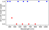 |
Fig. 6 LOO model weight of the CB model vs. the SH model for the Enceladus phase curves. When the model weight is close to 1, then the CB model is preferred (blue points), however close to 0 indicates that SH is preferred (red points). The red points show the phase curves where the SH model is confirmed. Bottom panel shows the LOO model weight plotted against the number of datapoints in each phase curve. There is a tentative negative correlation here, indicating that the more datapoints in a phase curve, the stronger the SH model is preferred. |
Enceladus phase curves’ preferred models.
Best-fit parameter results of the SH model fitting to Jupiter phase curves, including the priors used for the fitted parameters and the results of the derived parameters.
Best-fit parameter results of the SH model fitting to Enceladus phase curves, including the priors used for the fitted parameters and the results of the derived parameters.
3.3 FWHM as a solid surface detector
From previous studies (e.g. Dyudina et al. 2016), we see that one of the distinguishing features between the opposition effect from our Solar System objects is the ‘peaky-ness’ of the opposition maximum near zero phase. To quantify this, we used the best fit SH model to measure the FWHM (Equation (4)) of the different Jupiter and Enceladus phase curves and plotted them as a function of wavelength (see Figure 8).
We find the FWHM of Enceladus’ opposition peak to be an order of magnitude larger than Jupiter across the wavelength range. This helps quantify what we have seen in the rest of the Solar System, which is that the solid planets seem to have much smaller opposition FWHM peaks than the gaseous planet (Dyudina et al. 2016). This could be due to the difference in how light is scattered on a surface compared to within a gas. It could also be due to the dominant backscattering source or even the average distance between the scattering particles themselves.
4 Application to exoplanet phase curves
4.1 Rocky exoplanets
Characterising the climates of exoplanets is now one of the most important topics of research in the exoplanet field. Finding more methods to do this is therefore extremely valuable. We have so far proposed the possibility that measuring an opposition peak in the phase curve of a planet and then measuring the FWHM of this peak would be an indicator of whether the planet has a solid or gaseous surface.
In order to test whether this would be possible with an exoplanet, we ran a series of injection-recovery tests. Using a simulated phase curve of K2-141b, one of the most observable super-Earths (see, e.g. Barragán et al. 2018; Malavolta et al. 2018), we injected an Enceladus-like opposition peak using the best-fit parameters from our model fitting in Section 3.3. We took the SH model results since they were not ruled out by the data and as we only want to measure the FWHM of the peak, both the CB and SH fit should give the same result. Additionally, the formula for calculating the FWHM from the SH is easily given by Equation (4). We then adjusted the noise floor to simulate observations from both JWST and a future Habitable Worlds Observatory-like telescope. We took performance specifications from The LUVOIR Team (2019) as a starting point for the Habitable Worlds Observatory, and in-flight spectrophotometric precision measurements for JWST/NIRSpec from Mikal-Evans et al. (2023). We investigated how many observations are necessary to measure the injected (true) FWHM. Figure 9 shows the simulated phase curve (without the eclipse) with noise levels consistent with 103 and 105 JWST observations. From these fits we obtain the hSH posterior distribution, allowing us to calculate the FWHM as shown in Figure 10.
Our results are shown in Figure 10. We ran the test with two different simulated phase curves: one with and one without an eclipse present. This was important for us to test since an eclipse blocks the light from the planet near zero phase, exactly when the opposition peak signal is the strongest. Therefore we expect a present eclipse to make the fits less accurate than when we have all the data near zero phase. A phase curve with no eclipse could be produced by a non-transiting planet.
From our results we see that with JWST and a phase curve with an eclipse, it would take upwards of ∼106 phase curves in order to reach the precision necessary to reach FWHM measurements consistent with the true value. Using the lower predicted noise floor of Habitable Worlds, this decreases to ∼105 phase curves. Comparing these to the results when we use a phase curve with no eclipse present, the number of required observations significantly decreases. JWST requires ∼104 phase curves, whilst Habitable Worlds requires ∼103. Clearly both of these results show that this technique is not feasible with both current and planned future individual exoplanet observations. Perhaps it could still be used in the future for non-transiting exoplanets if a global population phase curve stacking technique was applied (e.g. Sheets & Deming 2017).
4.2 Jupiter-like exoplanets
We repeated the above injection and recovery test using simulated phase curves of HAT-P-7b and injecting them with an opposition-effect signal using the best fit parameters from the previous analysis on the Jupiter phase curves. We then used an MCMC fitting method to recover the hSH parameter (and therefore the FWHM) and compared this to the true value of the injected FWHM.
We find that both with and without an eclipse present in the phase curve, the number of observations required to contrain the FWHM is ∼102 lower than our previous investigation with a rocky exoplanet.
Since the FWHM we injected is much wider than the one we injected to mimic a rocky exoplanet, it has an effect over a larger range of phases, so more data contributes to constraining the opposition effect parameters, and fewer observations are needed. The second is that the orbital period is longer, so at a fixed exposure cadence, there are more observations per phase. Furthermore, the Rp/a for this type of planet is much larger than for the Enceladus-like planet (mostly due to the larger radius), increasing the amplitude of the phase curve and therefore our S/N. In Section 5.4, we investigated the parameter space of planetary orbital period and semi-major axis to see where the opposition signal would have the highest signal-to-noise (S/N).
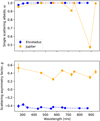 |
Fig. 7 Fitted values of the scattering asymmetry factor, g, and the single-scattering cross section, ω, across wavelength for Jupiter (orange) and Enceladus (blue). In the first panel, we see the single scattering albedo decrease (i.e. more absorption) around 750 and 900 nm for Jupiter, which is attributed to the methane absorption bands. We do not see this feature in Enceladus, since it has no considerable atmosphere. Both Jupiter and Enceladus show no trends in the asymmetry factors (second panel) across the wavelength range. This could imply, without taking into account surface roughness, that the size of the scattering particles are always equivalent to the wavelengths in this range, and therefore inhomogenous in these cases. For Enceladus, g is significantly lower, and negative, indicating that most of the light that hits the scattering particles (on the surface) is reflected backwards. This follows our intuition since Enceladus has an icy surface and no atmosphere, compared to Jupiter’s thick atmosphere and no solid surface. |
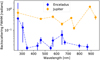 |
Fig. 8 Measured backscattering FWHM in the Jupiter (orange points) and Enceladus (blue points) phase curves. We find that there is generally an order of magnitude difference between the Enceladus and Jupiter measurements across the wavelength range. |
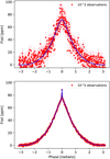 |
Fig. 9 Simulated phase curve model of K2-141b, a super-Earth (red points, with green errorbars). The blue line shows the best fit of our opposition effect model. The noise here is at a level consistent with 103 JWST observations (top panel) and 105 observations (bottom panel). |
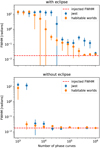 |
Fig. 10 Feasibility of detecting an Enceladus-like opposition effect signal in an exoplanet phase curve using both JWST and the future Habitable Worlds Observatory. The first panel shows the results when we use phase curves with an eclipse present and the second panel shows results without an eclipse present. The red line shows the FWHM value of the injected signal and the blue and orange points show the retrieved value, with 1σ errorbars. We find that, as expected, this signal is easier to detect in phase curves without an eclipse present, however this is still way beyond feasibility for both JWST and Habitable Worlds. |
5 Discussion
5.1 The effect of neglected surface properties on reflectance
The reflected light phase curve model in Section 2.2 describes a spherical planet built on formalism established in Hapke (1981) and extended in Heng et al. (2021). We adopted a parametrisation for shadow hiding from Hapke (2002), which implied that shadows are cast by topographical features that could be any optically thick obstruction to light, including mountains or clouds. The scale and shape of the shadow-casters was not parametrised in the model.
The full diversity of planetary surfaces in the Solar System cannot be described with shadow hiding or coherent backscat- tering, alone or in combination. Hapke (1984) established a parametrisation for reflected light phase curves with macroscopic roughness. Model lunar phase curves with surface roughness agreed well with observations after taking into account the distribution of surface slopes measured from lunar orbiters (Helfenstein 1988). Later work also established the effect of regolith porosity on phase curves (Hapke 2008).
A primary motivation for this study was to evaluate whether or not opposition surges are useful solid surface detectors for exoplanets. In Section 4.1, we showed that Enceladus-like opposition surges are unlikely to be measured in exoplanet phase curve observations in the foreseeable future. As such, we have not added further complexity to the models fit to the phase curves of Enceladus or Jupiter, since it is unlikely to affect the likelihood of opposition surge detections in exoplanets. Much higher precision phase curves are available elsewhere, and their precision requires the inclusion of these higher order effects in model fits. For example, Enceladus observations from Voyager and from the ground by Verbiscer & Veverka (1994) required macroscopic roughness to model the phase curve. Since the phase curve model here is parametrised through the single scattering albedo and scattering asymmetry parameter, the inferences for both parameters on Enceladus must be interpreted with these model limitations in mind. However, in, for example, Buratti & Veverka (1985), they found that topographical effects are not expected to be significant at phase angles less than 30–40◦, angles significantly larger than our focus for this study.
Despite our highly simplified model and wider phase angle coverage, the results presented in this work agree well with Verbiscer & Veverka (1994). Verbiscer & Veverka (1994) found ω = 0.999 ± 0.002 and ɡ = −0.39 ± 0.02, with opposition surge factor B0 = 0.21 ± 0.07. The Voyager instrument response with the clear filter has most transmittance between 400 and 600 nm, so the Cassini filter at 550 nm is likely the closest analogue in Table 4. We find smaller ɡ (−0.471 ± 0.007) and greater B0 (0.28 ± 0.01) in the Cassini 550 nm filter than the Voyager clear filter observations. The difference between solutions may be attributable to the difference in filter transmittance or the inclusion of regolith compaction in the analysis by Verbiscer & Veverka (1994). The small disagreement between parameters inferred in the two analyses is insufficient to change the outcome of the likelihood of opposition surge detection in exoplanets in Section 4.1.
5.2 Selecting an appropriate model
We fitted a set of reflected light phase curve models to Solar System observations. The scattering phase functions of these models are semi-empirical and constructed to fit observations of Solar System objects, but it is not clear from the theory which models should be applied to a given planet. Given the similarity of the model shapes, we have seen that trying to distinguish the preferred model (CB or SH) from the observations used in this study is very difficult. We could only tentatively conclude there was evidence for CB model being preferred for Jupiter. This of course does not rule out the possibility of both effects being present with one more dominant than the other or that the true solution is a different model entirely. For example, in Verbiscer et al. (2005), they found that for HST observations of Enceladus between 338 and 1022 nm, their best model was a combination of CB and SH, something that our work in Section 3.1 does not disagree with. However, as previously mentioned, our model does differ slightly from the model employed in Verbiscer et al. (2005) (see Section 2.2 for an overview of our model) so comparing these directly should be done with caution. Even for the Moon, where studies have been made on the Moon rock samples themselves, there are still many outstanding questions in regards to the contributions of CB and SH to the lunar opposition peak. There have been studies (see, e.g. Helfenstein et al. 1997) showing evidence that CB contributes to the peak at very small phase angles, and SH continues out to larger phase angles - however this is not conclusive. There is also very little investigation into the cause of the observed opposition effect on gaseous planets.
Furthermore, due to the known wavelength-dependence of some scattering properties, we expected some colourdependence in the best-fit parameters however this was not detected in our results. This could be due to the limited (and mostly optical) wavelength range where the albedo of these objects is both high. It has been seen in Buratti et al. (2022) that due to SH and CB acting differently on singly and multiply scattered light, the opposition surge form changes as you go to IR wavelengths. They hypothesise that this is due to the lower IR albedo reducing the influence of the multiply scattered light. However, due to our model formulation and since the forms for SH and CB are empirical and very similar (see, e.g. Section 3.1), the data we use is not precise enough to separate them and comment on this prediction.
However, due to SH and CB being direct outcomes of the scattering properties of the surface and/or atmosphere, unravelling these dependencies would provide information about the composition and particles on these planets.
5.3 Interpreting the best-fit parameters
For fitting our reflected light curves, we used, like other previous studies (see, e.g. Helfenstein et al. 1997; Heng & Li 2021), a single Henyey-Greenstein scattering phase function to describe the preferred scattering direction of an incoming ray to a scattering particle. This function includes the scattering asymmetry parameter, ɡ, which controls the amount of forward vs backward backscattering. When ɡ is close to 1 there is only forward scattering, whilst if ɡ is close to −1 then there is only backscattering present. Fitting for Enceladus, we derived a negative ɡ. This is more difficult to interpret since the scattering medium of Enceladus is a surface and not atmospheric gas. Therefore ɡ is harder to interpret in this scenario, which is not the medium the phase function was designed to model. Also, the scattering properties that can be derived from ɡ are probably not reliable for describing Enceladus’ suface. For Jupiter, since it has a large extended atmosphere, we believe this model is appropriate. Future works should take care in choosing the scattering phase function and be aware of its limitations in regards to solid bodies without atmospheres.
5.4 Optimal planet parameters for detecting the opposition effect
For a fixed planet radius Rp and opposition scattering parameters, two parameters dominate the S/N of the opposition peak: planetary orbital period and stellar mass. As the period increases, the number of datapoints per phase increases by the same amount. Therefore the S/N due to the number of datapoints goes as
 (7)
(7)
where Nexp is the number of exposures and P is the planetary orbital period. As the mass of the host star increases, by Kepler’s Third Law, the semi-major axis (a) also increases, for a fixed period. The amplitude of the reflected light phase curve of a planet is equal to Aɡ(Rp/a)2. Therefore the S/N goes as
 (8)
(8)
These show that the amplitude of the phase curve dominates how the S/N of the opposition peak changes with period. That is, as the period of the planet decreases, the S/N increases.
6 Conclusion
Reflected light phase curves of Solar System objects contain opposition peaks, which contain information about the surfaces where scattering occurs.
We fit Jupiter and Enceladus phase curves with a semi- empirical reflected light phase curve model and found that models with an opposition peak model are significantly preferred over simpler models, in agreement with previous Solar System work.
We showed that the FWHM of Jupiter’s opposition peak is an order of magnitude larger than that of Enceladus, uncovering the opportunity to differentiate solid from gaseous exoplanets using the FWHM of phase curve opposition peaks.
Cross-validation suggests a tentative preference for CB in Jupiter’s phase curve over SH, and a preference for SH in the phase curve of Enceladus.
We show that observations are unlikely to accurately measure the FWHM of a phase curve opposition peak in the next few decades, with either JWST or HWO
Appendix A Best fit results
We show here in Figure A.1 and A.2 the resulting posterior distributions of our fitted parameters during our analysis in Section 3.1.
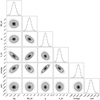 |
Fig. A.1 Corner plot showing the shadow hiding model best fit posteriors to the BL1 (463 nm) Jupiter phase curve, as shown in Figure 3. |
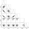 |
Fig. A.2 Corner plot showing the shadow hiding model best fit posteriors to the 798nm Enceladus phase curve, as shown in Figure 5. |
Appendix B Comparison to Heng & Li (2021)
This current analysis follows on from the work in Heng & Li (2021), where they tested different single scattering laws on a similar dataset from Li et al. (2018) of Jupiter phase curves. These phase curves not only consisted of observed data, but were interpolated so that they had homogeneous phase and wavelength coverage. We initially repeated our analysis in Section 3.1 with these interpolated phase curves. However we found this often led to bimodal solutions, which we speculated was an artifact of the interpolation procedure. Therefore we decided to use the original uninterpolated data in this analysis.
References
- Akkermans, E., Wolf, P., Maynard, R., & Maret, G. 1988, J. Phys. France 49, 77 [NASA ADS] [CrossRef] [EDP Sciences] [Google Scholar]
- Barragán, O., Gandolfi, D., Dai, F., et al. 2018, A&A, 612, A95 [Google Scholar]
- Bingham, E., Chen, J. P., Jankowiak, M., et al. 2019, J. Mach. Learn. Res., 20, 28 [Google Scholar]
- Buratti, B. J., & Veverka, J. 1985, Icarus, 64, 320 [NASA ADS] [CrossRef] [Google Scholar]
- Buratti, B. J., Hillier, J. H., Dalba, P. A., et al. 2022, Planet. Sci. J., 3, 200 [NASA ADS] [CrossRef] [Google Scholar]
- Dlugach, Z. M., & Mishchenko, M. I. 2013, Sol. Syst. Res., 47, 454 [CrossRef] [Google Scholar]
- Dyudina, U. A., Zhang, X., Li, L., et al. 2016, AAS/Div. Planet. Sci. Meeting Abst., 48, 202.08 [Google Scholar]
- Gehrels, T., Coffeen, T., & Owings, D. 1964, AJ, 69, 826 [NASA ADS] [CrossRef] [Google Scholar]
- Gelman, A., & Rubin, D. B. 1992, Stat. Sci., 7, 457 [Google Scholar]
- Hapke, B. 1981, J. Geophys. Res., 86, 4571 [NASA ADS] [Google Scholar]
- Hapke, B. 1984, Icarus, 59, 41 [Google Scholar]
- Hapke, B. 1986, Icarus, 67, 264 [Google Scholar]
- Hapke, B. 2002, Icarus, 157, 523 [NASA ADS] [CrossRef] [Google Scholar]
- Hapke, B. 2008, Icarus, 195, 918 [Google Scholar]
- Hapke, B. W. 1963, J. Geophys. Res., 68, 4571 [NASA ADS] [CrossRef] [Google Scholar]
- Hapke, B. W., Nelson, R. M., & Smythe, W. D. 1993, Science, 260, 509 [CrossRef] [Google Scholar]
- Hapke, B., Nelson, R., & Smythe, W. 1998, Icarus, 133, 89 [CrossRef] [Google Scholar]
- Helfenstein, P. 1988, Icarus, 73, 462 [NASA ADS] [CrossRef] [Google Scholar]
- Helfenstein, P., Veverka, J., & Hillier, J. 1997, Icarus, 128, 2 [NASA ADS] [CrossRef] [Google Scholar]
- Heng, K., & Li, L. 2021, ApJ, 909, L20 [NASA ADS] [CrossRef] [Google Scholar]
- Heng, K., Morris, B. M., & Kitzmann, D. 2021, Nat. Astron., 5, 1001 [NASA ADS] [CrossRef] [Google Scholar]
- Li, L., Jiang, X., West, R. A., et al. 2018, Nat. Commun., 9, 3709 [Google Scholar]
- Li, L., Guan, L., Li, S., et al. 2023, Icarus, 394, 115429 [NASA ADS] [CrossRef] [Google Scholar]
- Malavolta, L., Mayo, A. W., Louden, T., et al. 2018, AJ, 155, 107 [NASA ADS] [CrossRef] [Google Scholar]
- Mayorga, L., Jackiewicz, J., Rages, K., et al. 2016, AAS/Div. Planet. Sci. Meeting Abst., 48, 202.07 [Google Scholar]
- Mikal-Evans, T., Sing, D. K., Dong, J., et al. 2023, ApJ, 943, L17 [CrossRef] [Google Scholar]
- Morris, B. M., Heng, K., & Kitzmann, D. 2024, A&A, 685, A104 [NASA ADS] [CrossRef] [EDP Sciences] [Google Scholar]
- Phan, D., Pradhan, N., & Jankowiak, M. 2019, arXiv e-prints [arXiv:1912.11554] [Google Scholar]
- Sheets, H. A., & Deming, D. 2017, AJ, 154, 160 [CrossRef] [Google Scholar]
- Sudarsky, D., Burrows, A., Hubeny, I., & Li, A. 2005, ApJ, 627, 520 [NASA ADS] [CrossRef] [Google Scholar]
- The LUVOIR Team 2019, arXiv e-prints [arXiv:1912.06219] [Google Scholar]
- Vehtari, A., Gelman, A., & Gabry, J. 2015, arXiv e-prints [arXiv:1507.04544] [Google Scholar]
- Verbiscer, A. J., & Veverka, J. 1994, Icarus, 110, 155 [CrossRef] [Google Scholar]
- Verbiscer, A. J., French, R. G., & McGhee, C. A. 2005, Icarus, 173, 66 [NASA ADS] [CrossRef] [Google Scholar]
- von Seeliger, H. 1887, Abhandlungen der Bayerischen Akademie der Wissenschaften, Mathematisch-Naturwissenschaftliche Klasse, 16, 405 [Google Scholar]
All Tables
Best-fit parameter results of the SH model fitting to Jupiter phase curves, including the priors used for the fitted parameters and the results of the derived parameters.
Best-fit parameter results of the SH model fitting to Enceladus phase curves, including the priors used for the fitted parameters and the results of the derived parameters.
All Figures
|
Fig. 1 Jupiter Cassini phase curves from Li et al. (2018), with their corresponding colour filter used in this analysis. The datapoint colours are a crude guide for the different wavelengths of the filters. |
| In the text | |
|
Fig. 2 Enceladus Cassini phase curves from Li et al. (2023), with their corresponding colour filter used in this analysis. The datapoint colours are a crude guide for the different wavelengths of the filters. Some of the filters do not have alternative names. |
| In the text | |
|
Fig. 3 Best fit models to one of Jupiter’s phase curves (filter BL1, 463 nm) for three different models: a pure single Henyey-Greenstein model with no additional opposition peak, shadow hiding model, and coherent backscattering model. Top panel shows the three fits and the second panel shows the residuals of these best fits. It is clear that the model with no opposition peak is the worst fit to the data. The other two models produce, by eye, almost identical fits, which is expected since the functional forms are similar. However the residuals still show subtle differences. Using the LOO model selection statistic, we conclude that the coherent backscattering model is the best fitting model for this phase curve, along with all-but-one of the other Jupiter Cassini phase curves. The corner plot showing the posteriors for the shadow hiding model in this plot are in Appendix A, Figure A.1. |
| In the text | |
|
Fig. 4 LOO model weight of the CB model vs. the SH model for the Jupiter phase curves plotted against wavelength. When the model weight is close to 1, then the CB model is preferred (blue points), however close to 0 indicates that SH is preferred (red points). The red point shows the only phase curve where the SH model is preferred. |
| In the text | |
|
Fig. 5 Best fit models to one of one of Enceladus’ phase curves (filter 798 nm) for three different models: a pure single Henyey-Greenstein model with no additional opposition peak, shadow hiding model, and coherent backscattering model. Top panel shows the fits and the second panel shows the residuals of these best fits. It is clear that the model with no opposition peak is the worst fit to the data. The other two models produce, by eye, almost identical fits, which is expected since the functional forms are similar. However the residuals still show subtle differences. Using the LOO model selection statistic allows us to conclude that the coherent backscattering model is preferred by 7/12 of the phase curves, however not significantly. The corner plot showing the posteriors for the shadow hiding model are in Appendix A, Figure A.2. |
| In the text | |
|
Fig. 6 LOO model weight of the CB model vs. the SH model for the Enceladus phase curves. When the model weight is close to 1, then the CB model is preferred (blue points), however close to 0 indicates that SH is preferred (red points). The red points show the phase curves where the SH model is confirmed. Bottom panel shows the LOO model weight plotted against the number of datapoints in each phase curve. There is a tentative negative correlation here, indicating that the more datapoints in a phase curve, the stronger the SH model is preferred. |
| In the text | |
|
Fig. 7 Fitted values of the scattering asymmetry factor, g, and the single-scattering cross section, ω, across wavelength for Jupiter (orange) and Enceladus (blue). In the first panel, we see the single scattering albedo decrease (i.e. more absorption) around 750 and 900 nm for Jupiter, which is attributed to the methane absorption bands. We do not see this feature in Enceladus, since it has no considerable atmosphere. Both Jupiter and Enceladus show no trends in the asymmetry factors (second panel) across the wavelength range. This could imply, without taking into account surface roughness, that the size of the scattering particles are always equivalent to the wavelengths in this range, and therefore inhomogenous in these cases. For Enceladus, g is significantly lower, and negative, indicating that most of the light that hits the scattering particles (on the surface) is reflected backwards. This follows our intuition since Enceladus has an icy surface and no atmosphere, compared to Jupiter’s thick atmosphere and no solid surface. |
| In the text | |
|
Fig. 8 Measured backscattering FWHM in the Jupiter (orange points) and Enceladus (blue points) phase curves. We find that there is generally an order of magnitude difference between the Enceladus and Jupiter measurements across the wavelength range. |
| In the text | |
|
Fig. 9 Simulated phase curve model of K2-141b, a super-Earth (red points, with green errorbars). The blue line shows the best fit of our opposition effect model. The noise here is at a level consistent with 103 JWST observations (top panel) and 105 observations (bottom panel). |
| In the text | |
|
Fig. 10 Feasibility of detecting an Enceladus-like opposition effect signal in an exoplanet phase curve using both JWST and the future Habitable Worlds Observatory. The first panel shows the results when we use phase curves with an eclipse present and the second panel shows results without an eclipse present. The red line shows the FWHM value of the injected signal and the blue and orange points show the retrieved value, with 1σ errorbars. We find that, as expected, this signal is easier to detect in phase curves without an eclipse present, however this is still way beyond feasibility for both JWST and Habitable Worlds. |
| In the text | |
|
Fig. A.1 Corner plot showing the shadow hiding model best fit posteriors to the BL1 (463 nm) Jupiter phase curve, as shown in Figure 3. |
| In the text | |
|
Fig. A.2 Corner plot showing the shadow hiding model best fit posteriors to the 798nm Enceladus phase curve, as shown in Figure 5. |
| In the text | |
Current usage metrics show cumulative count of Article Views (full-text article views including HTML views, PDF and ePub downloads, according to the available data) and Abstracts Views on Vision4Press platform.
Data correspond to usage on the plateform after 2015. The current usage metrics is available 48-96 hours after online publication and is updated daily on week days.
Initial download of the metrics may take a while.