| Issue |
A&A
Volume 694, February 2025
|
|
|---|---|---|
| Article Number | A298 | |
| Number of page(s) | 8 | |
| Section | Planets, planetary systems, and small bodies | |
| DOI | https://doi.org/10.1051/0004-6361/202450850 | |
| Published online | 20 February 2025 | |
Collisional study of Hilda and quasi-Hilda asteroids
1
Instituto de Astrofísica de La Plata, CCT La Plata-CONICET-UNLP,
Paseo del Bosque S/N,
1900
La Plata,
Argentina
2
Facultad de Ciencias Astronómicas y Geofísicas, Universidad Nacional de La Plata,
Paseo del Bosque S/N,
1900
La Plata,
Argentina
3
Grupo de Ciencias Planetarias, Dpto. de Geofísica y Astronomía, FCEFyN, UNSJ – CONICET,
Av. J. I. de la Roza 590 oeste, J5402DCS Rivadavia,
San Juan,
Argentina
★ Corresponding author; This email address is being protected from spambots. You need JavaScript enabled to view it.
Received:
23
May
2024
Accepted:
15
January
2025
Abstract
Context. The Hilda asteroids are located in the outer main belt (MB) in a stable 3:2 mean-motion resonance (MMR) with Jupiter, while the quasi-Hildas have similar orbits but are not directly under the effect of the MMR. Moreover, cometary activity has been detected in quasi-Hildas.
Aims. In this study, we aim to investigate the collisional evolution of Hilda asteroids and apply it to an investigation into the cratering on asteroid (334) Chicago; we also intend to determine whether impacts between Hildas and quasi-Hildas can serve as a viable mechanism for inducing cometary activity.
Methods. Using the Asteroid Collisions and Dynamic Computation (ACDC) code, we simulated the collisional evolution of Hilda asteroids over a period of 4 Gyr. We considered three initial size-frequency distributions (SFDs) and two scaling laws for the collisional outcomes and performed a large set of simulations for each scenario, which we used to construct median SFDs of the Hilda population. We also derived an impactor SFD on asteroid (334) Chicago and used it to calculate the crater SFD on (334) Chicago. Additionally, we evaluated the sub-catastrophic impact timescale between Hilda and quasi-Hilda objects.
Results. The observed SFD of Hilda asteroids larger than 3 km is best matched by scenarios assuming that such an SFD is mostly primordial, implying minimal collisional activity over time. For smaller sizes, although unconstrained, the SFD steepens significantly due to the catastrophic fragmentation of a small number of multi-kilometre-sized bodies. We determined that the largest impactor on (334) Chicago measures a few kilometres in size, resulting in a maximum crater size of approximately 30 km. Furthermore, the slope of the crater SFD mirrors that of the initial SFD for sub-kilometric bodies. While impact events between Hildas and quasi-Hildas can induce observable activity, and although it is stochastic in nature, the timescale of such events exceeds the dynamical lifetime of quasi-Hildas, making them an unlikely primary mechanism for inducing observable activity.
Key words: methods: numerical / methods: statistical / minor planets, asteroids: general
© The Authors 2025
 Open Access article, published by EDP Sciences, under the terms of the Creative Commons Attribution License (https://creativecommons.org/licenses/by/4.0), which permits unrestricted use, distribution, and reproduction in any medium, provided the original work is properly cited.
This article is published in open access under the Subscribe to Open model. This email address is being protected from spambots. You need JavaScript enabled to view it. to support open access publication.
1 Introduction
The main asteroid belt (MB), located between the orbits of Mars and Jupiter, offers a significant opportunity to observe, study, and analyse the physical and dynamic mechanisms that have shaped the Solar System from its origin to its current state. The distribution of objects within the MB, particularly their depletion or accumulation in mean-motion resonances (MMRs) with Jupiter, underscores the predominant influence of Jupiter’s dynamics in shaping the structure of this region. The resonant structure of the MB has been extensively studied in the past (e.g. Nesvorný & Ferraz-Mello 1997; Nesvorný et al. 2002), primarily in order to comprehend the effects of MMRs and secular resonances on asteroid orbits and to explain conglomerations or gaps within the MB. Notably, certain MMRs with Jupiter, such as 3:1, 5:2, 7:3, and 2:1, as well as secular resonances such as ν6 and ν16, represent highly unstable zones that serve as pathways for asteroids to escape from the MB, particularly towards the near-Earth-object (NEO) region (e.g. Bottke et al. 2002; Granvik et al. 2017). Conversely, in other MMRs with Jupiter, such as 4:3, 3:2, and 1:1, there are asteroids whose stability persists further than the age of the Solar System (e.g. Nesvorný & Ferraz-Mello 1997; Levison et al. 1997).
In particular, the 3:2 MMR with Jupiter hosts the Hilda asteroids, constituting a numerous population whose critical angle  librates around 0°, where λJ denotes the mean longitude of Jupiter, and λ and
  represent the mean longitude and longitude of perihelion of the asteroid, respectively. Thus, when a Hilda asteroid is in conjunction with Jupiter, it is at perihelion, positioned far from Jupiter, which acts as a resonant protection mechanism. The Hilda group is centred at a semi-major axis of a = 3.97 au and is predominantly concentrated within a narrow fringe approximately 0.12 au wide around this value. This central region exhibits significant stability; however, it is surrounded by less stable regions where objects may escape from the resonance over the age of the Solar System (Ferraz-Mello et al. 1998; Nesvorný et al. 2002; Di Sisto et al. 2005). The primary mechanism for the removal of asteroids from the resonance is through collisions among Hildas, which can alter their orbital elements and critical angles; subsequently, this leads the asteroids into unstable regions, the resonance of which they may escape the altogether (Gil-Hutton & Brunini 2000).
Hilda asteroids are situated at the outer limit of the MB and exhibit physical properties similar to those of Jupiter Trojans. These predominantly belong to taxonomic classes D, P, and C (Dahlgren et al. 1997; DeMeo & Carry 2013), with Hildas being predominantly P-type by mass (DeMeo & Carry 2013).
Additionally, they have low albedos (Grav et al. 2012), rendering Hildas darker than Trojans by 15%–25% (Romanishin & Tegler 2018). Through an analysis of Sloan Digital Sky Survey (SDSS) colours, Gil-Hutton & Brunini (2008) and Wong & Brown (2017) found a clear bimodal spectral slope distribution among Hildas, delineating two distinct types of object: less red and red.
Due to their composition, which closely resembles that of Centaurs and comets, Hildas represent an interesting population for studying the physical and dynamic connections among various groups of small bodies within the Solar System. Particularly noteworthy are the quasi-Hildas located in the vicinity of the Hilda group. Some of these objects found in non-resonant orbits exhibit cometary activity (Kresak 1979; Gil-Hutton & García-Migani 2016; Correa-Otto et al. 2024), leading to their identification as comets. There are currently 26 known active quasi-Hildas. There are 20 reported by Toth (2006), which included the pre-capture orbits of D/SL9(1) and (2) and the encounter orbit of fragment D/SL9(D/1993 F2-K) and 39P/Oterma (1942 G1), since prior to its close encounter with Jupiter in 1963 it was a quasi-Hilda. The other objects are 212P (Cheng & Ip 2013), (457175) 2008 GO98 (Leonard et al. 2017; García-Migani & Gil-Hutton 2018), P/2010 H2 (Jewitt & Kim 2020), and 2008 QZ44 (Chandler et al. 2023), and, recently, 482P/2014 VF40 and 484P/2005 XR132 were reported active.
The quasi-Hilda region is part of the region inhabited by Jupiter-family comets (JFCs). However, this region also serves as an escape route for Hildas (Di Sisto et al. 2005), making it a compelling area in which to study physical and dynamical behaviours within the Solar System. It is therefore reasonable to expect that the quasi-Hilda region hosts both JFCs, originating from Centaurs and the trans-Neptunian region, and Hildas that have escaped from resonance. Detailed physical and dynamical studies of these objects, such as those conducted by Gil-Hutton & García-Migani (2016), García-Migani & Gil-Hutton (2018), and Correa-Otto et al. (2024), can provide valuable insights into their origins. However, the possibility remains that both Hildas and quasi-Hildas could undergo ‘activation’ due to mutual collisions (Jewitt et al. 2015). Given the ice content of Hildas, such activation could result in cometary activity. The discovery of active asteroids or MB comets as interlopers emphasises the connection between physical and dynamical processes within small body populations.
The collisional evolution and properties of Hildas, as well as outer MB asteroids, have been explored by Dahlgren et al. (1997); Gil-Hutton & Brunini (2000). These studies revealed a low level of current collisional activity, suggesting that the characteristics of large Hildas and the size-frequency distribution (SFD) are likely primordial. However, due to the significant increase in observed Hildas in recent years and the growing interest in their relationship with quasi-Hildas, we revisit the collisional study of this population. In this study, we investigated the collisional evolution of Hildas and quasi-Hildas with the objective of determining their SFD, analysing the distributions of impactors and craters on the largest Hilda asteroids, and estimating the impact frequency with quasi-Hildas to assess their potential for activation.
The paper is structured as follows. In Sect. 2, we present the observational data used and the construction of the observed SFDs. In Sect. 3, we briefly summarise the main properties and input parameters of the model and the scenarios we studied. In Sect. 4, we present our results of the collisional evolution of Hildas, the selection of runs, the final SFD, the impactor and crater distributions on the largest Hilda asteroids, and an estimation of the impact frequency with quasi-Hildas. Finally, the conclusions of this work and discussions on the results are presented in the last section.
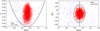 |
Fig. 1 Distribution of Hilda asteroids (depicted in red) and quasi-Hilda objects (depicted in blue) presented in the (a, e) plane (left) and (a, Φ) plane. The black ellipse in the left panel indicates the limits between the Hilda and quasi-Hildas regions, whereas the black curve in the right panel indicates the separatrix of the 3:2 MMR. |
2 Observational data
We initially aimed to construct cumulative SFDs of Hilda and quasi-Hilda asteroids, which we used to perform the collisional studies in this work. To achieve this, we retrieved the orbital elements and physical characteristics of all asteroids and comets in the outer MB from the Small-Body database query of the Jet Propulsion Laboratory (JPL)1 with 3.7 ≤ a ≤ 4.2 au. This initial sample comprises 6608 objects.
The orbital semimajor axis a and eccentricities e of these bodies are plotted in the left panel of Fig. 1. Almost all of the objects are located near the 3:2 MMR with Jupiter, at ∼3.9607 au, and inside the separatrix of the resonance (Murray & Dermott 2000); they are depicted via a black curve. In order to distinguish between Hilda and quasi-Hilda objects, we computed the resonant angle for all bodies:
 (1)
(1)
where λJ denotes the mean longitude of Jupiter, and λ and  represent the mean longitude and longitude of perihelion of the asteroid, respectively. The bodies located in the 3:2 MMR have Φ librating around 0°. The right panel of Fig. 1 shows the distribution of a and Φ for all the bodies. Following criteria similar to those of Correa-Otto et al. (2024), we define the Hilda population as the bodies located within the ellipse centred at a = 3.9067 au and Φ = 0° with amplitudes of ∆a = 0.07 au and ∆Φ = 125°, a value that corresponds to the 3σ criteria of the resonant angle distribution. Conversely, we define the quasi-Hildas as the bodies located outside the ellipse in the (a, Φ) plane.
Although JPL provides diameters and albedos for 1135 objects, the values for the rest are unknown. Thus, we utilised the diameters provided by JPL for bodies larger than 60 km. For smaller bodies and those without a measured albedo, we calculated the diameters from their absolute magnitude H using the following formula (Bowell et al. 1989):
![Mathematical equation: $D[{\rm{km}}] = {{1329} \over {\sqrt {p{\rm{V}}} }}{10^{ - H/5}},$](/articles/aa/full_html/2025/02/aa50850-24/aa50850-24-eq5.png) (2)
(2)
where pv denotes the visual albedo, which we assume to be 0.055 for Hildas and quasi-Hildas, a value obtained as the median of the albedos of Hilda asteroids provided by the JPL.
The largest asteroid in the region is (334) Chicago, with a diameter of 198.770 km (Mainzer et al. 2019), a semi-major axis of approximately 3.899 au, an eccentricity of approximately 0.025, and an inclination of approximately 4.68°2. (334) Chicago exhibits a significant value of the resonant angle Φ and frequently encounters Jupiter at close approach distances of approximately 1 au. Moreover, Ferraz-Mello et al. (1998) found that this asteroid’s orbit displays chaotic behaviour, as the resonant angle alternates between circulation and libration around 0°. It is located in a less stable region of the resonance, which increases the possibility of its escape from the region. However, its low eccentricity makes it highly unlikely to be a captured member of the JFC. Therefore, we consider the asteroid (334) Chicago as a member of the Hilda population, making it the largest body in the region.
Figure 2 illustrates the cumulative SFDs obtained for both populations. The SFD of Hilda objects exhibits a cumulative single-slope power law between 3 km and 60 km, with a slope of −2.03 being consistent with previous findings (Terai & Yoshida 2018) and similar to Jupiter’s Trojan asteroids (Marschall et al. 2022). At larger sizes, the slope appears to steepen, although this may be influenced by the limited number of objects. In contrast, the quasi-Hilda SFD does not show a uniform shape due to the reduced sample size, but it can be approximated by a power law with a slope of −1.35.
3 Collisional model
3.1 The ACDC code
In this study, we employed the Asteroid Collisions and Dynamic Computation (ACDC) code. ACDC is a statistical code designed to simulate the collisional and dynamical evolution of smallbody populations over a given integration time, in this case of 4 Gyr. The code was constructed following the outlines of previous collisional evolution models such as Bottke et al. (2005); Morbidelli et al. (2009); O’Brien & Greenberg (2005); de Elía & Brunini (2007) and Cibulková et al. (2014). In this section, we provide a concise overview of the fundamental aspects of the ACDC code. For an in-depth understanding of the construction and implementation of the model, we direct the reader to Zain et al. (2020).
The collisional component of the model is determined by tracking changes in the number of bodies resulting from objects being destroyed and fragments being ejected during collisions. In each timestep, ACDC calculates the number of collisions between all pairs of target-projectile bodies based on their intrinsic impact probabilities. Moreover, the occurrence of large impacts follows Poisson statistics. Subsequently, ACDC distributes the fragments created in each event over the different size bins and removes bodies that experience catastrophic disruption.
The dynamical component of the model, as implemented in previous works (Zain et al. 2020; Zain et al. 2021), incorporates the collective influence of the Yarkovsky effect and resonances. This mechanism serves to remove sub-kilometric asteroids from a specified region of the MB. However, the population examined in this study resides within an approximately 0.07 au half-width narrow region surrounding the 3:2 MMR with Jupiter. After conducting numerous tests, we found that the inclusion of the Yarkovsky effect leads to rapid depletion of this region, which appears to be independent of the physical, dynamical, and geometric properties of the asteroids within the studied area. Conversely, Brož & Vokrouhlickỳ (2008) investigated the dynamical evolution of asteroids initially positioned within the 3:2 MMR. Their findings suggest that the Yarkovsky effect within a strong first-order MMR primarily influences changes in orbital eccentricity, while the semi-major axis tends to follow the resonance centre. Given these considerations, we chose not to incorporate the Yarkovsky effect in this investigation.
We used ACDC to study the collisional evolution of the Hilda population. To do so, we considered collisions between targets and projectiles exclusively within the Hilda region, using the values for the intrinsic collision probability and impact velocity of 1.93 × 10⁻¹⁸ yr−1 km−2 and 3.36 km s−1, respectively (Dell’Oro et al. 2001).
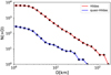 |
Fig. 2 Cumulative SFD of observed Hilda asteroids (red) and quasiHilda objects (blue). |
3.2 Scaling laws
The fundamental determinant of collision outcomes is the kinetic energy of the impact. Specifically, we employed the particular impact energy of the projectile:
 (3)
(3)
where mi and mj represent the masses of the target and impactor, respectively, and vimp is the mutual impact velocity.
The code compares Q with a function  , defined as the specific energy needed to disrupt and disperse 50% of the target mass. If a collision results in
  , it is labelled as a cratering event, while if
  , it is classified as a catastrophic disruption event. In either case, the code calculates the masses of the largest remnant, the largest fragment, and the cumulative SFD of the fragments following the relations derived by Benz & Asphaug (1999) and Durda et al. (2007). The collisional strength of the Hildas, represented by the function
  , is an unknown parameter. Therefore, in this study we adopted the functions derived by Benz & Asphaug (1999) for basaltic and icy targets at impact speeds of 5 km s−1 and 3 km s−1, respectively.
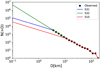 |
Fig. 3 Initial SFD tested for Hilda asteroids, labelled as S31, S10, and S32. Black dots indicate the observed SFD for Hilda asteroids larger than 3 km. |
3.3 Initial Hilda SFD
The shape of the initial SFD of the Hilda asteroids is also an unknown property. However, insights from previous collisional and dynamical studies suggest that Hilda populations may be very old and that collisional activity has been minimal (Gil-Hutton & Brunini 2000; Davis et al. 2002; Brož et al. 2011). Consequently, we assume that the SFD for sizes larger than 10 km is primordial.
For smaller sizes, we adopted the approach outlined in the collisional study of Jupiter’s Trojan asteroids of Marschall et al. (2022) due to their physical similarities and common origin with Hilda asteroids (Terai & Yoshida 2018). We propose three distinct scenarios for the initial Hilda SFD, illustrated in Fig. 3: S32, where the initial slope below 3 km continues the observed slope from 3 to 10 km; S31, where the slope below 3 km is set to 1; and S10, where the slope below 10 km is also set to 1, resulting in a shallower slope than for the observed population. For each scenario, we conducted two sets of 20 000 simulations, employing the scaling laws for icy and basaltic targets as described by Benz & Asphaug (1999).
4 Results
4.1 Collisional evolution of Hildas
In this section, we present the results on the collisional evolution of the Hilda population over 4 Gyr. One of the main features of ACDC is its high level of stochasticity, treating large impacts as random events through the application of Poisson statistics. Consequentially, runs using different random seeds may produce varied results. To address this variability, we performed an extensive set of 20 000 runs for each scenario and for each scaling law. Then, we applied observational constraints to identify and interpret the most robust results statistically. In this particular study, the only observational constraint considered is the Hilda SFD for sizes larger than 3 km, as shown in Fig. 2.
To quantitatively assess the fidelity of a simulation in replicating observational data, we followed the methodology outlined by Bottke et al. (2005). We define a metric designed to evaluate the goodness of fit between the observed SFD, denoted as Nobs, and the simulated SFD, denoted as Nsim:
 (4)
(4)
where the summation extends over size bins ranging from 3 km to 100 km. We calculated ψ2 for each simulation, where a lower value of ψ2 indicates better alignment with the observational data. Figure 4 illustrates the distribution of metrics among the runs performed in each scenario. In particular, scenario S32 exhibits the lowest metrics, with 80% of runs yielding ψ2 values below 0.2. Following closely is scenario S31, where 80% of runs result in ψ2 values smaller than 1. For comparison, Bottke et al. (2005) suggests that a simulation provides a good fit if ψ2 < 20. The S10 scenario is capable of producing good fits but in a much smaller quantity. We find that approximately 1% of the runs produce good fits according to the criteria of Bottke et al. (2005), with values of ψ2 between 2 and 20. In all cases, we observe that the distribution of the metrics remains consistent regardless of whether we consider  for icy or basaltic targets.
We utilised the ψ2 metrics to select the runs that offer the best fits. The SFD obtained from these runs is used to construct a representative median SFD for sizes ranging from 10 cm to 200 km by calculating the median number of objects in each size bin using the individual SFDs that meet the given selection criteria. For scenarios S31 and S32, we included simulations with ψ2 ≤ 1, while for the S10 scenario we included those with ψ2 < 20 following the criteria of Bottke et al. (2005).
The median SFDs are depicted in Fig. 5. We note that scenarios S31 and S32 exhibit nearly exact fits with the observed SFD for sizes larger than 3 km. These scenarios were formulated under the assumption that the observed SFD in that size range is primordial, suggesting that minimal catastrophic collisional activity occurred in the multi-kilometre-sized Hilda asteroids over 4 Gyr. The S10 scenario, which did not initially match the observed SFD, was still able to generate an imperfect but acceptable fit within the observed range. However, it is worth recalling that this median was constructed using significantly fewer runs than the other two scenarios.
The median SFD diverges from the initial populations in the sub-kilometre size range, where we lack observational constraints to distinguish between them. However, we can utilise our median SFDs in the mentioned size range to address the general behaviour. The top left panel of Fig. 6 illustrates the median SFD with icy and basaltic targets. Remarkably, the distributions obtained with the different scaling laws are nearly identical for the S31 and S32 scenarios, possibly due to the generally low collisional activity in the region. In the S31 scenario, both SFD distributions exhibit slight differences in the metre size range, where the SFD for icy bodies is slightly lower than the SFD for basaltic bodies. Furthermore, all scenarios exhibit steeper slopes than the initial populations, implying a general increase in the number of small bodies. These slopes have values of 2.59 and 2.54 for S31 and 32, respectively, indicating a state of near collisional equilibrium (Dohnanyi 1969). This increase in the SFD is further highlighted in the top right panel of Fig. 6, which presents the ratio between the median and the initial SFD. In the S32 scenario, the median SFD is approximately ten times higher than the initial SFD for bodies larger than 10 cm, and it decreases to 1 for bodies larger than 20 m for icy targets and 100 m for basaltic targets. The increase in numbers is much more pronounced in the S31 scenario, where the ratio increases to 104 for bodies larger than 10 cm and decreases to 1 in the kilometre range. Conversely, Fig. 6 illustrates that the collisional activity was more intense in the S10 scenario. On one hand, the left panel reveals that the median SFD exhibits a more pronounced wavy shape compared to the other scenarios. On the other hand, the right panel shows that the ratio between the median and initial SFD extends to multi-kilometre-sized bodies and increases with decreasing size until reaching 106 for centimetre-sized bodies. Furthermore, the SFDs and ratios obtained with the different scaling laws exhibit differences of over an order of magnitude.
The model utilised in this study lacks any dynamical mechanism for the removal of small bodies. Consequently, the increase in the number of bodies suggests that the Hilda SFD in the sub-kilometre range is solely influenced by the catastrophic fragmentation of larger bodies. The bottom left panel of Fig. 6 illustrates the SFD of catastrophically disrupted bodies larger than 100 m, while the bottom right panel shows the ratio of catastrophically disrupted bodies with respect to the initial SFD.
We observe that the highest number of catastrophic collisions occur in the S32 scenario, resulting in 3 × 10³ destroyed bodies larger than 100 m, which represent only 10−3 of the initial SFD. Conversely, the number of catastrophic collisions is much lower in the S31 scenario, where only 25 and ten bodies larger than 100 m and 1 km, respectively, are disrupted, representing up to ∼10−3 of the initial SFD. In both the S31 and S32 scenarios, the largest catastrophically disrupted body has a size of 6 km, and the results are very similar regardless of the scaling law considered. The number of catastrophic collisions is even smaller for the S10 scenario, where only ten bodies larger than 100 m are catastrophically disrupted. However, since this scenario is much less common in general terms, the catastrophic collisions represent a larger fraction of the initial population, reaching values up to 3 × 10⁻². The number of catastrophic collisions is even smaller for the S10 scenario, where only ten bodies larger than 100 m are catastrophically disrupted. Additionally, we find that the S10 scenario results in the disruption of larger bodies than the other two scenarios, with the largest disrupted body having a size of 22 km and 35 km for the ice and basalt scaling laws, respectively. Indeed, as the number of catastrophic collisions is low, this results in a higher number of projectiles in the SFD capable of disrupting larger bodies.
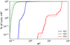 |
Fig. 4 Distribution of ψ2 across 20 000 runs in each scenario. The x-axis represents ψ2 values, while the y-axis depicts the percentage of runs with values below the corresponding ψ2 threshold. Solid lines indicate the results for the ice scaling law, while dashed lines represent the results for the basalt scaling law. |
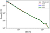 |
Fig. 5 Median SFD of Hilda asteroids larger than 1 km after 4 Gyr of collisional evolution for the S10 (red), S31 (blue), and S32 (green) scenarios. Black dots indicate the observed SFD size in kilometres. |
4.2 Impactors and cratering on the largest Hilda asteroid
Using ACDC, it is possible to record the number of collisions of projectiles on bodies from a given size bin during the integration time of 4 Gyr. We utilised this to obtain a median SFD of impactors larger than 1 m on the largest asteroid in the Hilda region using the runs selected in the previous section. This particular asteroid is discussed in Sect. 2 and is called (334) Chicago. It has a diameter of ∼200 km and is classified as a C-type asteroid according to Tholen taxonomy. We obtain that it was not hit by large bodies. In particular, the largest impactor has sizes of 1.77 km, 1.41 km, and 2.24 km for the S10, S31, and S32 scenarios, respectively.
With this information, we can derive an SFD for the number of craters produced by these impacts. To calculate the apparent transient crater diameter dt resulting from a projectile of diameter d, we employed the scaling law proposed by Holsapple & Housen (2007):
![Mathematical equation: ${d_{\rm{t}}} = {K_1}{\left[ {\left( {{{gd} \over {2v_i^2}}} \right){{\left( {{{{\rho _t}} \over {{\rho _i}}}} \right)}^{{{2v} \over \mu }}} + {K_2}{{\left( {{Y \over {{\rho _t}v_i^2}}} \right)}^{{{2 + \mu } \over \mu }}}{{\left( {{{{\rho _t}} \over {{\rho _i}}}} \right)}^{{{\nu (2 + \mu } \over \mu }}}} \right]^{ - {\mu \over {2 + \mu }}}}d,$](/articles/aa/full_html/2025/02/aa50850-24/aa50850-24-eq13.png) (5)
(5)
where ρt = 1.5 g cm−3 is the target density, ɡ its surface gravity, Y its strength, ρi the density of the impactor that we assume is the same as ρt, and vi the impactor velocity. The two exponents µ and ν and the constants K1 and K2 characterise the target material. Following our previous work where we calculated the crater SFD for Ceres (Zain et al. 2021), we used K1 = 1.67; K2 = 0.8; µ = 0.38 and ν = 0.378; and Y = 4 × 10⁶ dyn cm−2 (Kraus et al. 2011; Di Sisto & Zanardi 2013; Hiesinger et al. 2016). The final crater size is obtained by multiplying Eq. (5) by 1.3k, with k = 1.19 (Marchi et al. 2011).
The crater SFDs for the three scenarios are shown in Fig. 7. The largest craters, represented as dots in the figure, measure 30 km, 24 km, and 37 km in the S10, S31, and S32 scenarios, respectively. Remarkably, the crater distributions exhibit notable differences. While the S10 and S31 distributions overlap across all size ranges, the S32 scenario displays a considerably higher number of craters, spanning several orders of magnitude compared to the other two scenarios. However, it is noteworthy that the slope observed in the three crater distributions mirrors the slope of their respective initial SFDs for sub-kilometre bodies. This observation could provide a valuable constraint for future observational efforts aimed at determining the initial distribution of Hilda asteroids, should a space mission targeting Hilda asteroids be developed. Nevertheless, it is essential to emphasise that this study does not account for possible impacts with bodies from other populations such as the MB, Jupiter Trojans, JFCs, or early planetesimals. Also, we neglect the effect of crater saturation, as the small number of impacts makes it unlikely for the surfaces to become saturated.
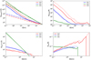 |
Fig. 6 Evolution of the SFD of Hilda asteroids relative to the initial population. Top: median SFD (left) and ratio with respect to the initial SFD in the sub-kilometre size range for the S10 (red), S31 (blue), and S32 (green) scenarios. Dashed-dotted lines represent the initial SFD. Bottom: SFD of catastrophically disrupted bodies (left) and ratio of catastrophically disrupted bodies with respect to the initial SFD (right) for the S10 (red), S31 (blue), and S32 (green) scenarios. Solid lines represent simulations conducted with icy targets’ scaling laws, while dashed lines indicate simulations with basaltic targets. |
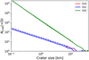 |
Fig. 7 SFD of craters on surface of asteroid (334) Chicago, the largest member of the Hilda asteroids, for the S10 (red), S31 (blue), and S32 (green) scenarios. Circles indicate the size of the largest crater. Solid lines depict the results for the ice scaling law, while dashed lines represent the results for the basalt scaling law. |
4.3 Impacts and observable activity on quasi-Hildas
In this section, we discuss the contribution of impacts to quasiHildas in terms of their observable activity. To accomplish this, we utilised the expression derived by Jewitt et al. (2015), which provides the minimum radius of a projectile rp required to create ejecta with a substantial cross-section when impacting a target of radius rt:
 (6)
(6)
where vesc denotes the escape velocity of the asteroid, U = 3.34 km s−1 represents the impact velocity (Dell’Oro et al. 2001), A = 0.01 and α = −1.5 are parameters from Housen & Holsapple (2011), and a = 0.1 mm is specified by Jewitt et al. (2015). The parameter f relates the mass of the ejecta to the scattering cross-section and to changes in the apparent magnitude. We adopted a value of f = 1, which, as indicated by Jewitt et al. (2015), would lead to an approximate doubling of the asteroid’s brightness, making it readily detectable. According to Jewitt et al. (2015), even modest impacts can produce observable ejecta signatures. In fact, employing Eq. (6), we find that an impact of a 30 cm projectile on a 1 km asteroid would eject enough material to double the brightness post impact. Similarly, a 45 m projectile would have the same effect by impacting a 10 km asteroid.
We estimated the occurrence of impact-triggered quasi-Hilda activity by calculating the frequency of sub-catastrophic collisions between quasi-Hildas and Hildas. To do so, we made the simple assumption that both populations share the same impact speeds and probabilities. We considered targets from the quasiHilda population with sizes ranging from 1 km to 14 km. The projectiles are Hilda asteroids, which follow the SFD obtained from collisional evolution in this study in the different scenarios. We utilised the SFDs obtained using the ice scaling law, as Eq. (6) requires both the target and the projectile to have the same density. The frequency is then calculated as
 (7)
(7)
where P = 1.93 × 10⁻¹⁸ yr−1 km−2 is the intrinsic collision probability (Dell’Oro et al. 2001), and Np denotes the number of Hilda projectiles with diameter Dp. The summation extends from a minimum value of 2rp (as per Eq. (6)) to a maximum size of (2Q*/U2)1/3Dt, which corresponds to the projectile size capable of catastrophically disrupting the targets (Bottke et al. 2005).
In the top panel of Fig. 8, we plot the impact timescales calculated as the inverse of the frequencies calculated from Eq. (7). It is evident that the difference in the timescales between each scenario is approximately an order of magnitude, reflecting the difference in the number of bodies at the smaller end of the SFDs. The timescales are shorter in the S32 scenario, where the SFD in Fig. 6 shows almost 1014 objects larger than 10 cm. Consequently, a quasi-Hilda object with sizes between 2 km and 4 km experiences one impact every 1.6 × 10⁶ years, which increases to 5 × 10⁶ years for targets larger than 7 km. The impact timescales exhibit a similar trend, with one and two orders of magnitude larger timescales for the S10 and S31 scenarios, respectively.
It is worth noting that while the frequencies and timescales are calculated based on deterministic laws, the occurrence of impacts on quasi-Hilda asteroids is stochastic due to the low number of objects in these regions. Specifically, we only have 20 objects larger than 10 km in the quasi-Hilda region. Nevertheless, we find that these timescales are many orders of magnitude longer than the dynamical lifetimes of objects in the quasiHilda region. We calculated from previous studies that objects, whether escaped Hildas as described in Di Sisto et al. (2005) or JFCs as mentioned in Di Sisto et al. (2009), spend a few thousand years traversing the region, eventually reaching up to approximately 5 × 10⁵ years. Additionally, García-Migani & Gil-Hutton (2018) identified the object (457175) as a quasi-Hilda for a duration of 7 × 10⁴ years. Overall, our analysis indicates that the frequency of impacts capable of inducing activity on quasiHildas is too low for collisions between Hildas and quasi-Hildas to be deemed a primary mechanism.
Nevertheless, it should be noted that the vast majority of quasi-Hildas observed to be active display their activity in the post-perihelion arc. This suggests that thermal processes primarily trigger activity that is generally not initiated solely due to the thermal inertia of the object. In other words, the collision of a projectile causing fragments to increase the reflective surface and thus brightening may not be the preferential process (Vincent et al. 2015). Cometary ice transforms into compact amorphous ice down to depths of approximately 10–20 m due to Galactic cosmic rays (Maggiolo et al. 2020). Cosmic rays also contribute to the formation of a refractory mantle, requiring the outermost layer of a comet to be broken in order to expose ices and facilitate sublimation. Consequently, collisions occurring in quasi-Hildas could potentially disrupt or penetrate the outermost layer, leaving the comet’s ice vulnerable. Subsequently, upon passing through perihelion, the comet resumes its thermal sublimation cycle.
To assess the frequency of collisions capable of producing a crater that can penetrate the outermost comet layer and expose ices, we consider a depth of h = 10 m. The relationship between depth h and diameter D of a crater for asteroids has a mean value of h/D = 0.15 (Marchi et al. 2015). Thus, we need to consider craters with D = 66 m. Using Eq. (5), we determine that the impactor producing such a crater on 1–15 km targets has a size of approximately 4 m. We used Eq. (7), starting the summation from 4 m, and plot the timescale in the bottom panel of Fig. 8. We find that the timescale increases significantly at the small end due to the limited range of impactor sizes considered. However, for larger bodies, the set of possible impactor sizes expands, resulting in a slight reduction in the timescale. The shortest timescale is associated with the S32 scenario, reaching down to 2 × 10⁶ years, but it still exceeds the dynamic lifetimes of quasi-Hildas in the region.
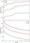 |
Fig. 8 Timescale of sub-catastrophic impacts capable of producing observable activity on quasi-Hildas for the S10 (red), S31 (green), and S32 (blue) scenarios. The top panel indicates the timescale for impacts onto a single quasi-Hilda target, while the bottom panel indicates the timescale of impacts from projectiles capable of forming a 10 m deep crater and exposing the ice beneath the surface. |
5 Conclusions and discussions
In this work, we performed a collisional study of the Hilda asteroids and their potential for activating quasi-Hildas through impacts. Here, we summarise our key findings:
We obtained the SFDs of the observed Hilda and quasiHilda populations. The SFD of the Hilda population exhibits a cumulative slope of −2.03, which is similar to that of Jupiter’s Trojan asteroids. In contrast, the quasi-Hilda SFD displays a two-slope power law, with a slope of −2.4 for bodies between 3 km and 6 km, and a −1.21 for bodies between 6 km and 20 km;
We explored the collisional evolution of Hilda asteroids over a 4 Gyr period. We found that scenarios assuming minimal catastrophic collisional activity in the multi-kilometre-sized Hilda asteroids produced the best fits to the observed SFDs. The slopes of the initial SFDs for sub-kilometre-sized bodies were found to steepen over time due to the fragmentation of a small number of multi-kilometric sized bodies;
We analysed the impactor and cratering events on the largest member of the Hilda asteroids, (334) Chicago. Our results show that this asteroid experienced minimal impacts from large bodies over the integration period. The largest crater produced on this asteroid is between 20 and 32 km in size. Moreover, the crater SFD reflects the slope of the initial SFD in the sub-kilometre range. Therefore, a mission aimed at observing this asteroid and in particular the craters on its surface would be of utmost importance to restrict the original population of the Hildas and their origin;
Impacts on quasi-Hildas can lead to observable activity, with even modest collisions capable of doubling the brightness of these objects. However, the timescale of impact-triggered activity is notably larger than the dynamical lifetime of quasi-Hildas. Despite their potential to induce activity and the stochastic nature of such events, the collisions between Hildas and quasi-Hildas are unlikely to be a primary mechanism for the observed phenomena.
The results of this study reaffirm the findings of previous works in the literature regarding the limited overall evolution experienced by the Hilda asteroids. However, it is important to note that this analysis was conducted considering only collisions between Hilda asteroids. Other small-body populations, such as the Jupiter Trojans or MB asteroids, may also interact collisionally with Hilda and quasi-Hilda objects, although the intrinsic collisional probability with these populations is an order of magnitude lower than that between Hilda objects (Dahlgren 1998; Dell’Oro et al. 2001). On one hand, the contribution of the Jupiter Trojan population may be neglected. We can estimate a timescale of impacts between pairs of Hilda targets of DH in size and Trojan projectiles of DT in size as the inverse of  , with Pi = 0.27 × 10⁻¹⁸ yr−1 km−2 (Dell’Oro et al. 2001). N(> DT) is the SFD of the Trojan population (Di Sisto et al. 2019), which is assumed to be primarily primordial in the multi-kilometre size range (Marschall et al. 2022). Based on this, the catastrophic collisions with Trojan projectiles capable of substantially modifying the Hilda SFD occur on timescales comparable to the age of the Solar System, while small cratering impacts occur on timescales of over 107 years. On the other hand, the contribution from the MB could be assessed within the context of a study focused on the collisional evolution of the MB itself, which is beyond the scope of this work. This is a non-trivial matter, as the MB is a large and complex structure with distinct physical and dynamical properties, and it can be divided into at least three regions: the inner, middle, and outer belts (de Elía & Brunini 2007; Cibulková et al. 2014; Zain et al. 2020). This is particularly relevant for the Hilda population, as its members are more likely to collide with bodies from the outer MB, given that the mean perihelion distance of Hilda objects is approximately 3.13 au. Specifically, a collisional evolution study focused on the outer MB could provide the currently unconstrained SFD in the sub-kilometre size range, which is necessary for calculating the impact timescales between outer MB asteroids and quasi-Hildas. This represents an interesting area for future research on the collisional evolution of small Solar System bodies.
Acknowledgements
This research was performed using computational resources of Facultad de Ciencias Astronómicas y Geofísicas de La Plata (FCAGLP) and Instituto de Astrofísica de La Plata (IALP), and received partial funding from Universidad Nacional de La Plata (UNLP) under PID G172. RGH gratefully acknowledges financial support by CONICET through PIP 112-202001-01227 and San Juan National University by a CICITCA grant for the period 2023–2024.
References
- Benz, W., & Asphaug, E. 1999, Icarus, 142, 5 [NASA ADS] [CrossRef] [Google Scholar]
- Bottke, W. F., Morbidelli, A., Jedicke, R., et al. 2002, Icarus, 156, 399 [NASA ADS] [CrossRef] [Google Scholar]
- Bottke, W. F., Durda, D. D., Nesvorný, D., et al. 2005, Icarus, 175, 111 [Google Scholar]
- Bowell, E., Hapke, B., Domingue, D., et al. 1989, in Asteroids II, eds. R. P. Binzel, T. Gehrels, & M. S. Matthews, 524 [Google Scholar]
- Brož, M., & Vokrouhlicky, D. 2008, MNRAS, 390, 715 [CrossRef] [Google Scholar]
- Brož, M., Vokrouhlicky, D., Morbidelli, A., Nesvorny, D., & Bottke, W. 2011, MNRAS, 414, 2716 [CrossRef] [Google Scholar]
- Chandler, C. O., Oldroyd, W. J., Trujillo, C. A., et al. 2023, RNAAS, 7, 271 [NASA ADS] [Google Scholar]
- Cheng, Y. C., & Ip, W. H. 2013, ApJ, 770, 97 [NASA ADS] [CrossRef] [Google Scholar]
- Cibulková, H., Brož, M., & Benavidez, P. G. 2014, Icarus, 241, 358 [CrossRef] [Google Scholar]
- Correa-Otto, J., García-Migani, E., & Gil-Hutton, R. 2024, MNRAS, 527, 876 [Google Scholar]
- Dahlgren, M. 1998, A&A, 336, 1056 [NASA ADS] [Google Scholar]
- Dahlgren, M., Lagerkvist, C. I., Fitzsimmons, A., Williams, I. P., & Gordon, M. 1997, A&A, 323, 606 [NASA ADS] [Google Scholar]
- Davis, D. R., Durda, D. D., Marzari, F., Campo Bagatin, A., & Gil-Hutton, R. 2002, Asteroids III, 545 [CrossRef] [Google Scholar]
- de Elía, G. C., & Brunini, A. 2007, A&A, 466, 1159 [NASA ADS] [CrossRef] [EDP Sciences] [Google Scholar]
- Dell’Oro, A., Marzari, F., Paolicchi, P., & Vanzani, V. 2001, A&A, 366, 1053 [CrossRef] [EDP Sciences] [Google Scholar]
- DeMeo, F. E., & Carry, B. 2013, Icarus, 226, 723 [NASA ADS] [CrossRef] [Google Scholar]
- Di Sisto, R. P., & Zanardi, M. 2013, A&A, 553, A79 [NASA ADS] [EDP Sciences] [Google Scholar]
- Di Sisto, R. P., Brunini, A., Dirani, L. D., & Orellana, R. B. 2005, Icarus, 174, 81 [NASA ADS] [CrossRef] [Google Scholar]
- Di Sisto, R. P., Fernández, J. A., & Brunini, A. 2009, Icarus, 203, 140 [Google Scholar]
- Di Sisto, R. P., Ramos, X. S., & Gallardo, T. 2019, Icarus, 319, 828 [NASA ADS] [CrossRef] [Google Scholar]
- Dohnanyi, J. S. 1969, J. Geophys. Res., 74, 2531 [Google Scholar]
- Durda, D. D., Bottke, W. F., Nesvorný, D., et al. 2007, Icarus, 186, 498 [NASA ADS] [CrossRef] [Google Scholar]
- Ferraz-Mello, S., Nesvorny, D., & Michtchenko, T. A. 1998, in Astronomical Society of the Pacific Conference Series, 149, Solar System Formation and Evolution, eds. D. Lazzaro, R. Vieira Martins, S. Ferraz-Mello, & J. Fernandez, 65 [NASA ADS] [Google Scholar]
- García-Migani, E., & Gil-Hutton, R. 2018, Planet. Space Sci., 160, 12 [CrossRef] [Google Scholar]
- Gil-Hutton, R., & Brunini, A. 2000, Icarus, 145, 382 [NASA ADS] [CrossRef] [Google Scholar]
- Gil-Hutton, R., & Brunini, A. 2008, Icarus, 193, 567 [NASA ADS] [CrossRef] [Google Scholar]
- Gil-Hutton, R., & García-Migani, E. 2016, A&A, 590, A111 [NASA ADS] [CrossRef] [EDP Sciences] [Google Scholar]
- Granvik, M., Morbidelli, A., Vokrouhlicky, D., et al. 2017, A&A, 598, A52 [NASA ADS] [CrossRef] [EDP Sciences] [Google Scholar]
- Grav, T., Mainzer, A. K., Bauer, J., et al. 2012, ApJ, 744, 197 [NASA ADS] [CrossRef] [Google Scholar]
- Hiesinger, H., Marchi, S., Schmedemann, N., et al. 2016, Science, 353, aaf4758 [NASA ADS] [CrossRef] [Google Scholar]
- Holsapple, K. A., & Housen, K. R. 2007, Icarus, 187, 345 [NASA ADS] [CrossRef] [Google Scholar]
- Housen, K. R., & Holsapple, K. A. 2011, Icarus, 211, 856 [NASA ADS] [CrossRef] [Google Scholar]
- Jewitt, D., & Kim, Y. 2020, Planet. Sci. J., 1, 77 [NASA ADS] [CrossRef] [Google Scholar]
- Jewitt, D., Hsieh, H., Agarwal, J., et al. 2015, Asteroids IV, 221 [Google Scholar]
- Kraus, R. G., Senft, L. E., & Stewart, S. T. 2011, Icarus, 214, 724 [NASA ADS] [CrossRef] [Google Scholar]
- Kresak, L. 1979, in Asteroids, eds. T. Gehrels, & M. S. Matthews, 289 [Google Scholar]
- Leonard, G., Christensen, E., Fuls, D., et al. 2017, Minor Planet Electronic Circulars, 2017 [Google Scholar]
- Levison, H. F., Shoemaker, E. M., & Shoemaker, C. S. 1997, Nature, 385, 42 [NASA ADS] [CrossRef] [Google Scholar]
- Maggiolo, R., Gronoff, G., Cessateur, G., et al. 2020, ApJ, 901, 136 [NASA ADS] [CrossRef] [Google Scholar]
- Mainzer, A. K., Bauer, J. M., Cutri, R. M., et al. 2019, NASA planetary data System, https://doi.org/10.26033/18S3-2Z54 [Google Scholar]
- Marchi, S., Massironi, M., Cremonese, G., et al. 2011, Planet. Space Sci., 59, 1968 [NASA ADS] [CrossRef] [Google Scholar]
- Marchi, S., Chapman, C. R., Barnouin, O. S., Richardson, J. E., & Vincent, J. B. 2015, in Asteroids IV, 725 [Google Scholar]
- Marschall, R., Nesvorny, D., Deienno, R., et al. 2022, AJ, 164, 167 [NASA ADS] [CrossRef] [Google Scholar]
- Morbidelli, A., Bottke, W. F., Nesvorný, D., & Levison, H. F. 2009, Icarus, 204, 558 [Google Scholar]
- Murray, C. D., & Dermott, S. F. 2000, Solar System Dynamics (Cambridge University Press) [Google Scholar]
- Nesvorný, D., & Ferraz-Mello, S. 1997, Icarus, 130, 247 [CrossRef] [Google Scholar]
- Nesvorný, D., Ferraz-Mello, S., Holman, M., & Morbidelli, A. 2002, in Asteroids III, 379 [CrossRef] [Google Scholar]
- O’Brien, D. P., & Greenberg, R. 2005, Icarus, 178, 179 [CrossRef] [Google Scholar]
- Romanishin, W., & Tegler, S. C. 2018, AJ, 156, 19 [NASA ADS] [CrossRef] [Google Scholar]
- Terai, T., & Yoshida, F. 2018, AJ, 156, 30 [NASA ADS] [CrossRef] [Google Scholar]
- Toth, I. 2006, A&A, 448, 1191 [NASA ADS] [CrossRef] [EDP Sciences] [Google Scholar]
- Vincent, J.-B., Bodewits, D., Besse, S., et al. 2015, Nature, 523, 63 [Google Scholar]
- Wong, I., & Brown, M. E. 2017, AJ, 153, 69 [NASA ADS] [CrossRef] [Google Scholar]
- Zain, P. S., de Elia, G. C., & Di Sisto, R. P. 2020, A&A, 639, A9 [NASA ADS] [CrossRef] [EDP Sciences] [Google Scholar]
- Zain, P. S., Di Sisto, R. P., & de Elía, G. C. 2021, A&A, 652, A122 [NASA ADS] [CrossRef] [EDP Sciences] [Google Scholar]
All Figures
|
Fig. 1 Distribution of Hilda asteroids (depicted in red) and quasi-Hilda objects (depicted in blue) presented in the (a, e) plane (left) and (a, Φ) plane. The black ellipse in the left panel indicates the limits between the Hilda and quasi-Hildas regions, whereas the black curve in the right panel indicates the separatrix of the 3:2 MMR. |
| In the text | |
|
Fig. 2 Cumulative SFD of observed Hilda asteroids (red) and quasiHilda objects (blue). |
| In the text | |
|
Fig. 3 Initial SFD tested for Hilda asteroids, labelled as S31, S10, and S32. Black dots indicate the observed SFD for Hilda asteroids larger than 3 km. |
| In the text | |
|
Fig. 4 Distribution of ψ2 across 20 000 runs in each scenario. The x-axis represents ψ2 values, while the y-axis depicts the percentage of runs with values below the corresponding ψ2 threshold. Solid lines indicate the results for the ice scaling law, while dashed lines represent the results for the basalt scaling law. |
| In the text | |
|
Fig. 5 Median SFD of Hilda asteroids larger than 1 km after 4 Gyr of collisional evolution for the S10 (red), S31 (blue), and S32 (green) scenarios. Black dots indicate the observed SFD size in kilometres. |
| In the text | |
|
Fig. 6 Evolution of the SFD of Hilda asteroids relative to the initial population. Top: median SFD (left) and ratio with respect to the initial SFD in the sub-kilometre size range for the S10 (red), S31 (blue), and S32 (green) scenarios. Dashed-dotted lines represent the initial SFD. Bottom: SFD of catastrophically disrupted bodies (left) and ratio of catastrophically disrupted bodies with respect to the initial SFD (right) for the S10 (red), S31 (blue), and S32 (green) scenarios. Solid lines represent simulations conducted with icy targets’ scaling laws, while dashed lines indicate simulations with basaltic targets. |
| In the text | |
|
Fig. 7 SFD of craters on surface of asteroid (334) Chicago, the largest member of the Hilda asteroids, for the S10 (red), S31 (blue), and S32 (green) scenarios. Circles indicate the size of the largest crater. Solid lines depict the results for the ice scaling law, while dashed lines represent the results for the basalt scaling law. |
| In the text | |
|
Fig. 8 Timescale of sub-catastrophic impacts capable of producing observable activity on quasi-Hildas for the S10 (red), S31 (green), and S32 (blue) scenarios. The top panel indicates the timescale for impacts onto a single quasi-Hilda target, while the bottom panel indicates the timescale of impacts from projectiles capable of forming a 10 m deep crater and exposing the ice beneath the surface. |
| In the text | |
Current usage metrics show cumulative count of Article Views (full-text article views including HTML views, PDF and ePub downloads, according to the available data) and Abstracts Views on Vision4Press platform.
Data correspond to usage on the plateform after 2015. The current usage metrics is available 48-96 hours after online publication and is updated daily on week days.
Initial download of the metrics may take a while.