| Issue |
A&A
Volume 694, February 2025
|
|
|---|---|---|
| Article Number | A22 | |
| Number of page(s) | 10 | |
| Section | Atomic, molecular, and nuclear data | |
| DOI | https://doi.org/10.1051/0004-6361/202450295 | |
| Published online | 30 January 2025 | |
Depolarization and polarization transfer rates for the C2 (X1 Σ+g, a 3Πu) + H(2S1/2) collisions in the solar photosphere
1
Astronomy and Space Science Department, Faculty of Science, King Abdulaziz University,
PO Box 80203,
Jeddah
21589,
Saudi Arabia
2
Department of Optics and Spectroscopy, Tomsk State University,
36 Lenin av.,
Tomsk
634050,
Russia
3
Institute of Spectroscopy, Russian Academy of Sciences,
Fizicheskaya St. 5,
108840
Troitsk, Moscow,
Russia
★ Corresponding author; This email address is being protected from spambots. You need JavaScript enabled to view it.
Received:
8
April
2024
Accepted:
31
December
2024
Abstract
Context. This paper is a continuation of a series of studies that investigated the collisional depolarization of solar molecular lines such as those of MgH, CN and C2. It is focused on the solar molecule C2, which exhibits striking scattering polarization profiles, although its intensity profiles are inconspicuous and barely visible. The current interpretation of the C2 polarization in terms of magnetic fields is incomplete because collisional data are almost completely lacking.
Aims. We accurately compute the collisional depolarization and polarization transfer rates for the C2(X1Σg+,α3Πu) by isotropic collisions with hydrogen atoms H (2S l/2). We also investigate the solar implications of our findings.
Methods. We used the package MOLPRO to obtain potential energy surfaces for the electronic states X1Σg+ and a3Πu of C2, and the code MOLSCAT to study the quantum dynamics of the C2(X1Σg+,α3Πu) + H(2S1/2) systems. We used the tensorial irreducible basis to express the resulting collisional cross sections and rates. Furthermore, sophisticated genetic programming techniques were employed to determine analytical expressions for the temperature and total molecular angular momentum dependence of these collisional rates.
Results. We obtained quantum depolarization and polarization transfer rates for the C2(X1Σg+,α3Πu) + H(2S1/2) collisions in the temperature range T = 2000−15 000 K. We also determined analytical expressions that write these rates as functions of the temperature and total molecular angular momentum. In addition, we show that isotropic collisions with neutral hydrogen can only partially depolarize the lower state of the C2 lines. This highlights that the approximation of neglecting lower-level polarization is limited in modeling the polarization of C2 lines.
Conclusions. Isotropic collisions with neutral hydrogen atoms are a fundamental ingredient for understanding C2 polarization.
Key words: line: formation / molecular data / molecular processes / polarization / Sun: magnetic fields / Sun: photosphere
© The Authors 2025
 Open Access article, published by EDP Sciences, under the terms of the Creative Commons Attribution License (https://creativecommons.org/licenses/by/4.0), which permits unrestricted use, distribution, and reproduction in any medium, provided the original work is properly cited.
This article is published in open access under the Subscribe to Open model. This email address is being protected from spambots. You need JavaScript enabled to view it. to support open access publication.
1 Introduction
Highly sensitive spectropolarimetric telescopes have opened new observation windows on the lines of MgH, CN, and C2 molecules with unprecedented spatial and spectral resolutions (e.g., Stenflo 1994; Gandorfer 2000; Berdyugina et al. 2002; Faurobert & Arnaud 2003; Berdyugina & Fluri 2004; Asensio Ramos & Trujillo Bueno 2005; Trujillo Bueno et al. 2006; Milić & Faurobert 2012; Wiegelmann et al. 2014; Wöger et al. 2021). Furthermore, the Hanle effect on molecular polarized solar lines provides a good opportunity to determine spatially unresolved magnetic fields given the diverse magnetic sensitivities of the molecular lines that are observed within narrow spectral regions. The observation and interpretation of the molecular C2 lines of the Swan system (d3Πu−a3Πu) around 5141 Å constitute an interesting tool for inferring the magnetic field strength (e.g., Berdyugina & Fluri 2004; Milić & Faurobert 2012). Nevertheless, some discrepancies have been found in the results regarding magnetic field strengths (e.g., Asensio Ramos & Trujillo Bueno 2005; Derouich et al. 2006; Kleint et al. 2010). To eliminate a primary cause of these discrepancies, the effect of collisions on the formation of molecular lines should be taken into account. The main difficulty for all Hanle diagnostics of the molecular lines is that the collisional rates are poorly known.
In particular, collisions with the hydrogen atom are of great importance due to its high density in the photosphere, where the Hanle effect acts. The precise determination of magnetic fields is significantly affected when collisions are ignored because collisions compete with the Hanle depolarizing effect of the turbulent photospheric magnetic fields. To contribute to addressing this difficulty, Qutub et al. (2020, 2021) calculated the collisional depolarization and polarization transfer rates of the ground states of the MgH and CN molecules by collisions with hydrogen atoms for the first time. In a continuation of this effort, we compute the depolarization and transfer of polarization rates for the two lowest-energy electronic states of C2 due to collisions with hydrogen atoms here.
As C2 is a homonuclear molecule, no transitions between rotational levels with different parities can occur (see, e.g., Flower 1990; Derouich 2006). This restriction arises from the symmetry of the interaction potential. However, this does not imply that the C2 molecule is immune to collisions. As demonstrated in this paper, collisional transitions between rotational levels with the same parity can affect the polarization of the C2 electronic levels, and consequently, they affect the polarization of the C2 solar lines (e.g., Kleint et al. 2010). In this regard, we calculated the depolarization and polarization transfer rates of the solar C2 molecules in their ground- and first excited states  and a3Πu due to collisions with H atoms in their ground state 2S1/2.
The first step of this calculation was to determine the potential energy surfaces (PESs) for H+C2 interactions. All the PESs were obtained using the package MOLPRO (e.g., Werner et al. 2010). The second step was determining the collision dynamics by solving the corresponding Schrödinger equations. The dynamics calculations were made possible by the code MOLSCAT (e.g., Hutson & Green 1994). Then, the depolarization and polarization transfer cross sections were computed within the tensorial basis  where k is the tensorial order, and q quantifies the coherence within the molecular level. These cross sections are independent of q because the collisions are isotropic. We adopted the infinite-order sudden (IOS) approximation to calculate the cross sections for kinetic energies ranging from 50 to 40 000 cm−1 and calculated the depolarization and polarization transfer rates for temperatures ranging from T = 2000 to 15 000 K. Finally, genetic programming methods were applied to infer useful analytical expressions of the obtained rates. In addition, the expected solar implications of our results are briefly discussed below. The computed cross sections are publicly available on Zenodo for future use by the community.
2 Potential energy surfaces
We considered the ground  and the first excited a3Πu electronic states of C2 molecule, which are close in energy and are separated by approximately 700 cm−1 (i.e., ~0.087 eV) (see, e.g., Martin 1992). When C2
  interacts with the hydrogen atom H in its 2S ground electronic state, the resultant system can exist in one electronic state 1 2A′. Additionally, 2 2A′ and 2 2A″ represent the two states that result from the interaction between C2(a3Πu) and H (2S). We adopted the coordinate system of Jacobi (R,
  , θ) to calculate the PESs. The intermolecular vector R connects the center of mass of the C2 molecule and the hydrogen atom. The angle θ defines the rotation of the hydrogen atom around the C2 molecule. We assumed the C2 molecule to be a rigid rotor, and we froze the C–C distance at its equilibrium value
  a0 (Huber & Herzberg 1979). This is justified under solar physical conditions, where the rates for vibrational excitations due to collisions are much lower than those for pure rotational excitations.
Ab initio calculations of the PESs for the electronic states of C2–H system, described above, were carried out using the multireference configuration interaction wave functions including Davidson correction (MRCI+Q) (see Langhoff & Davidson 1974; Davidson & Silver 1977; Werner & Meyer 1981; Wener & Knowles 1988). The computations were performed using the package MOLPRO 2010 (e.g., Werner et al. 2010).
For the electronic states under consideration, the twodimensional PESs were generated for an angle θ ranging from 0 to 90° with variable steps to accurately capture their behavior, and for R values ranging from a0 to 50 a0 . We used 84 values of R (a0 ≤ R ≤ 50 a0) and 51 values of θ (0° ≤ θ ≤ 90°), implying that the total number of the generated ab initio points was 4284 for each potential surface V(R, θ). Because C2 is a homonuclear molecule, the interaction potential V is invariant under the exchange of the two carbon atoms, that is, V(R, θ) = V(R, 180°− θ). The PES of the electronic state 1 2A′, resulting from C2 and H (2S) interaction, is shown in Figure 1. Furthermore, the PESs of the 2 2A′ and 2 2A″ states represented in Figure 2 result from the interaction between C2(a3Πu) and H (2S).
The PES corresponding to the state 1 2A′ reaches its minimum at R ~ 3.2 a0 and θ ~ 0°, with an energy of E ~−41 000 cm−1. The PESs corresponding to the state 2 2A′ and 22A″ states have a similar minimum energy E ~−39 000 cm−1, with θ~0° and R~ 3.2 a0.
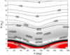 |
Fig. 1 Contour plot of the PES of the electronic state 1 2A′ as a function of R and θ. The energy is plotted in cm−1. |
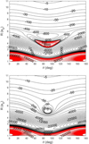 |
Fig. 2 Contour plots of the PESs of the electronic states 2 2A′ (upper panel) and 2 2A″ (lower panel) as functions of R and θ. The energy is plotted in cm−1 . |
3 Collisional problem
In the context of the close-coupling (CC) scheme, it is very difficult to generate comprehensive results for the depolarization and polarization transfer rates of the C2 molecule because of the numerous rotational levels, the spin characteristics, and the large number of possible k-values for each rotational level. To overcome this difficulty, we adopted the IOS approximation, which is appropriate for solar temperatures, to treat the collision problem, and we provide comprehensive data for all collisional rates. As we are interested in the solar context, where the temperature and the kinetic energies of collisions are sufficiently high, we expect that some simplification regarding the coupling effects should be invoked in order to obtain results with an acceptable accuracy in a reasonable calculation time.
We adopted the formalism developed by Corey & Alexander (1985), which is based on the decoupling of the rotational-orbital motion from the atomic and molecular spin angular momenta (see also Corey & McCourt 1983). This decoupling scheme offers an advantage in our attempt to express the tensorial cross sections in terms of the generalized IOS cross sections, especially for the case of C2(a3Πu) state, where the orbital angular momentum and the spin of the molecule are nonzero. In a collision between an open-shell molecule (e.g., C2 a3Πu) and an open-shell target (e.g., H2S), the PESs are dependent on the total spin of the composite atom-molecule system, and this dependence was taken into account in the PESs calculations. However, we neglected the effect of the spin of hydrogen in the collision dynamics, and we only considered the molecular spin, which is a further approximation necessary for expressing the tensorial cross sections factorized into products of terms involving the IOS cross sections. In these conditions, (see Equations (13a,b,c) of Corey & Alexander 1985)
 (1)
(1)
where ℛ is the rotational angular momentum of the diatomic C2 molecule and Sd is its spin; Sd = 0 for  and Sd = 1 for a3Πu. L is the electronic orbital momentum of the molecular state; L = 0 for
  and L = 1 for a3Πu. We note that N is the total rotational-orbital angular momentum, and j is the total momentum of the molecule, taking the spin into account.
In the framework of the coupling scheme given in Equation (1), by following a method similar to that explained in various works concerned with molecule–atom collisions, and by including the IOS approximation (e.g., Pack 1972, 1974; Alexander & Davis 1983; Alexander & Dagdigian 1983; Corey & Alexander 1985; Corey et al. 1986; Corey & Smith 1985; Werner et al. 1989; Follmeg et al. 1990; Green 1994; Dagdigian & Alexander 2009a,b,c; Paterson et al. 2009; McGurk et al. 2012), we show that
 (2)
(2)
where E is the kinetic energy, and  are the IOS polarization transfer cross sections from the level (ℛNj) to (ℛ′N′j′) within the electronic state el, and σ(el, 0 → K, E) are the generalized IOS cross sections. From the general formula in Equation (2), the limiting case can be recovered where Sd = L = 0 (see, e.g., Derouich 2006; Lique et al. 2007).
The depolarization cross section of the level (ℛNj) is given by
 (3)
(3)
where  (el, j → j, E) is obtained from Equation (2) with j = j′, ℛ = ℛ′, and N = N′.
To resolve the collision dynamics of the problem at hand under the IOS approximation, the PESs were introduced into the code MOLSCAT (e.g., Hutson & Green 1994). As a result, we obtained the generalized IOS cross sections σ(el, 0 → K, E) for energies 50 ≤ E (cm−1) ≤ 40 000 and 0 ≤ K ≤ 158 (K is even). The data giving σ(el, 0 → K, E) for all E and K values and for el = a3Πu and  , are made accessible on Zenodo. For each PES, we obtained the IOS cross sections σ(el, 0 → K, E), so that we obtained σ(1 2A′, 0 → K, E) for the PES corresponding to the 12A′ state resulting from C2
  and H(2S) interaction, that is,
 (4)
(4)
while σ(22 A′, 0 → K, E) and σ(22 A″, 0 → K, E) were obtained by solving the collision dynamics after introducing the PESs of the 22A′ and 2 2A″ states, respectively. 22A′ and 2 2A″ result from the interaction between C2(a3Πu) and H (2S) and have the same spin. Thus, the cross sections corresponding to the C2(a3Πu) + H (2S) are given by
 (5)
(5)
The  (el, j →j′, E) were then obtained by applying Equation (2). The depolarization rates
 (6)
(6)
of the level (ℛNj) due to elastic collisions and the polarization transfer rates Dk (el, j →j′, T) between the levels (ℛNj) and (ℛ′N′ j′) due to inelastic collisions were obtained by thermally averaging the respective IOS cross sections,
 (7)
(7)
for temperatures in the range 2000–15 000 K. Here, nH is the density of the incident hydrogen atoms, kB is the Boltzmann constant, and є = E/kBT.
In the case of homonuclear molecules such as C2, no collisional transitions between levels with even and odd j-values (or ℛ-values in the considered decoupling scheme) can occur (see, e.g., Flower 1990; Derouich 2006). This restriction is related to the symmetry of the interaction potential, where V(R, θ) = V(R, 180° − θ) (see Section 2). This clearly does not mean that the C2 molecule is immune to collisions. Collisional transitions with ∆ j (or ∆ℛ in our case) even are allowed, which constitute a possibility of a collisional contribution to the statistical equilibrium equations (SEE) given by
![Mathematical equation: $\eqalign{ & {\left( {{{{d^j}\rho _q^k} \over {dt}}} \right)_{coll{\rm{ }}}} = - \left[ {{D^k}(j,T)} \right. \cr & {\left. {\,\,\,\,\,\,\,\,\,\,\,\,\,\,\,\,\,\,\,\,\,\,\,\,\,\,\,\,\, + \sum\limits_{{j^\prime } \ne j} {\sqrt {{{2{j^\prime } + 1} \over {2j + 1}}} } {D^0}\left( {j \to {j^\prime },T} \right)} \right]^j}\rho _q^k \cr & \,\,\,\,\,\,\,\,\,\,\,\,\,\,\,\,\,\,\,\,\,\,\,\,\,\,\,\,\, + \sum\limits_{{j^\prime } \ne j} {{D^k}} {\left( {{j^\prime } \to j,T} \right)^{{j^\prime }}}\rho _q^k, \cr} $](/articles/aa/full_html/2025/02/aa50295-24/aa50295-24-eq26.png) (8)
(8)
where  are the density matrix elements expressed in the ten- sorial basis, which allow us to describe the internal states of the C2 molecule (e.g., Sahal-Bréchot 1977; Landi Degl’Innocenti & Landolfi 2004). The importance of the collisional effects is mainly associated with the value of nH and to a lesser extent, with T. In the case of isotropic collisions, the transfer of polarization rates obeys the detailed balance relation
 (9)
(9)
where Ej is the energy of the level (j).
4 Results
We have determined polarization transfer rates Dk (j → j′, T) and depolarization rates Dk(j, T) associated with rotational levels within the C2 electronic states  and a 3Πu. When possible, genetic programming (GP) fitting techniques were employed to express these rates as two-variable functions, with the variables being j, which varied from 0 to 60, and T, which extended from 2000 to 15 000 K. The GP fits can be expressed in the following general analytical form:
 (10)
(10)
where the GP coefficients  and
and  are provided in Tables A.1–A.6 of Appendix A. As representative examples, we provide Dk(j → j′, T) and Dk(j, T) for six cases. However, Equation (2) can be used to derive any other case by incorporating the quantum numbers of interest and summing over the generalized IOS cross sections σ(0 → K, E), which are conveniently accessible on Zenodo. When the cross sections are obtained, an average over the energies should be performed to obtain the rates (see Equation (7)). This enables nonspecialized readers to obtain cross sections or collisional rates for any C2 rotational level within the electronic states
  and a 3Πu.
4.1 Results for the X1Σ+ g-state
Figure 3 shows the variation in the collisional depolarization rates Dk(j, T) for the alignment (k = 2) and orientation (k = 1) as functions of j at T = 6000 K in the upper panel and as functions of T for the level Nj = 66 in the lower panel. The depolarization rates with tensorial order k = 2 are higher than those with tensorial order k = 1, as observed in Figure 3. As expected, the Dk (j, T) rates increase with temperature (for a given j) and decrease with increasing j (for a given T) (see, e.g., Derouich 2006). The  rates determined using Equation (10) and Table A.1 are shown as solid curves in Figure 3, demonstrating excellent agreement with the Dk(j, T) rates computed directly. The percentage error in the
  values is smaller than 5% for any j and T in the considered ranges.
In the upper panel of Figure 4, we set ∆ j = j′ − j = 2 and T = 6000 K, and we show the dependence of the excitation (i.e., Ej′ > Ej) transfer on the polarization rates Dk(j → j′, T) for k = 0, 1, and 2 as functions of j. The solid curves in the upper panel of Figure 4 agree very well for the directly calculated values and the GP fit values obtained using Equation (10) and Table A.2. The percentage difference between the real calculated values and the GP values is smaller than 5%. As shown in the upper panel of Figure 4, the Dk (j → j′ = j + 2, T) rates increase rapidly with j for low values of j and vary slowly for sufficiently large j. Thus, Dk(j→j′ = j + 2, T) can be considered practically constant for sufficiently high j values. In the lower panel of Figure 4, we illustrate that the rates Dk (j→j′, T) decrease quickly with increasing (j′− j) for the level Nj = 66 and T = 6000 K.
0 (open diamonds), k = 1 (open triangles), and k = 2 (open circles) is shown in the upper panel as functions of j for j′ − j = 2 and T = 6000 K, and as functions of (j′ − j) for the level Nj = 66 and T = 6000 K in the lower panel. The solid curves in the upper panel show the GP fit values obtained using Equation (10) and Table A.2.
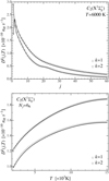 |
Fig. 3 Collisional depolarization rates, Dk(j, T), for C2 rotational levels within the electronic states |

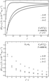 |
Fig. 4 Collisional transfer rates, Dk(j → j′, T), for C2 rotational levels within the electronic states |

4.2 Results for the a 3Πu-state
For the electronic state a3Πu, with a molecular spin Sd = 1, j can take values of N −1, N, or N +1. As illustrated in the upper panel of Figure 5, for j ≳ 5, the depolarization rates, Dk(j, T), decrease with increasing j at constant temperature. Additionally, the depolarization rates increase as T increases for constant j, as shown in the lower panel of Figure 5. We note that the depolarization rates with tensorial order k = 2 are higher than those with tensorial order k =1. This is also the case for the state  . Using the GP fitting techniques, we obtained analytical expressions for Dk(j, T) rates. These expressions are given by Equation (10) for the temperature range 2000–15 000 K and for total angular momentum j from 1 to 60. The GP coefficients are provided in Tables A.3, A.4 and A.5 for j = N − 1, j = N and j = N + 1, respectively. The percentage error in the GP rates
  is smaller than 5%.
Figure 6 shows the rates of polarization transfer associated with C2 rotational levels within the electronic states a 3Πu. The upper panel of Figure 6 illustrates a significant increase in the transfer rates Dk (j → j′ = j+2, T) as j increases for sufficiently small j. For j ≳ 20, the transfer rates continue to increase with increasing j, but at a slower rate. This result gives interesting insights into the differential effect of collisions when comparing the polarization of molecular lines with different j-values. For lines involving levels with sufficiently large j, the Dk(j → j′ = j + 2, T) can be considered practically constant, which greatly simplifies the modeling. This is also the case for the electronic state  .
.
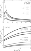 |
Fig. 5 Collisonal depolarization rates, Dk(j, T), for C2 rotational levels in electronic states a3Πu. The upper panel illustrates the rates for k = 1 (open markers) and k = 2 (solid markers) with respect to j at T = 6000 K, where j = N−1 (circles), j = N (rectangles), and j = N +1 (triangles) are displayed. The lower panel shows the temperature variation in the rates for k = 1 (open markers) and k = 2 (solid markers) with the different j values of the N = 13 multiplet. Both panels display the fit values (dotted, dashed, and solid curves) we obtained using Equation (10) and GP coefficients of Tables A.3, A.4, and A.5. |
5 Use of the IOS approach in collision dynamics
Unlike the CC methods, which are both time-intensive and require case-by-case calculations, the IOS approach allows us to derive comprehensive tables that contain generalized IOS cross sections. These tables facilitate the efficient generation of collisional rates for all transitions and tensorial orders k with good accuracy, in particular at solar temperatures (T ≳ 5000 K).
To assess the validity of the IOS approximation, we carried out a CC calculation of the cross sections using the PES of the interaction  for kinetic energies up to 5000 cm−1, which allowed us to calculate collisional rates for temperatures up to 1300 K with an accuracy better than a few percent. In Figure 7, we compare the IOS rate to the CC rate for the collisional rotation transition j = 6 → j′ = 4. The IOS collisional rate, which is lower at low temperatures, converges to the CC collisional rate as the temperature increases; the difference between the two rates becomes smaller than 5% for T = 1300 K (see Figure 7). For higher temperatures, in particular, for solar temperatures, the difference should be negligibly small. This is also expected to hold true for the PESs arising from interaction between C2(a3Πu) and H (2S).
We also compared our IOS collisional rotational deexcitation cross sections, obtained with our PES for  , to the corresponding coupled-state cross sections of Najar et al. (2014), which they calculated using their own PES. In particular, at an energy of approximately 350 cm−1, we find that
for the transition j = 2 → j′ = 0, our cross section is 1.53 Å2, while the cross section of Najar et al. (2014) is about 2 Å2, and
for j = 4 → j′ = 0, our cross section is 0.75 Å , while the cross section of Najar et al. (2014) is about 0.8 Å2.
The differences are smaller than 25% at these relatively low energies and are expected to become negligible for the higher energies that contribute to the rates at temperatures above 2000 K, which are the focus of this paper. Najar et al. (2014) did not consider energies above 350 cm−1, and therefore, a comparison at higher energies is not possible.
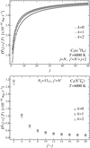 |
Fig. 6 Collisional transfer rates, Dk ( j → j′, T), for C2 rotational levels within the electronic states a 3Πu. The upper panel shows variation with j of the rates for k = 0 (open diamonds), k = 1 (open triangle), and k = 2 (open circles), where we have set j′ – j = 2 and T = 6000 K. The solid curves show the GP fit values obtained using Equation (10) and GP coefficients of Table A.6. The lower panel displays the variation in the rates with ( j′ - j) for k = 0 (open diamonds), k = 1 (open triangle), and k = 2 (open circles), where we set T = 6000 K, Nj = 1313, and j′ = N′. |
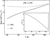 |
Fig. 7 Comparison between the IOS rate (solid curve) and the CC rate (dashed curve) for the collisional rotational deexcitation, j = 6 → j′ = 4 as functions of temperature. Additionally, the inset shows the percent-difference between the two rates. The percent-difference |

6 Solar implications
Observations of the second solar spectrum (SSS) revealed the existence of prominent linear polarization signals due to lines of the C2 molecule (e.g., Gandorfer 2000; Faurobert & Arnaud 2003; Gandorfer et al. 2004; Kleint et al. 2008). Furthermore, theoretical analyses pointed out the suitability of these lines for the application of the differential Hanle effect to study variations in the turbulent magnetic fields in the photosphere where the C2 line region forms around 5141 Å (e.g., Berdyugina & Fluri 2004; Kleint et al. 2010, 2011; Milić & Faurobert 2012). Nevertheless, these theoretical studies faced the problem of a total lack of collisional rates, which impacted the accuracy of their conclusions.
We considered the implication of our results for the molecular C2 lines of the Swan system (d3Πu–a3Πu). In particular, we selected the triplet R1(14), R2(13) and R3 (12) of the R-branch and the P-triplet P1(42), P2(41), P3(40), which are suitable for solar magnetic field diagnostics (see Kleint et al. 2010). To estimate the effect of isotropic collisions, we compared the collisional depolarization rates D2( j, T) of the lower state a3Πu for a typical photospheric hydrogen density (nH = 1015–1016 cm−3) to the inverse lifetime (1/tlife = BℓuI(λℓu)) of the lower levels of the R-triplet and P-triplet lines. Here, I(λℓu) denotes the intensity of light with a wavelength λℓu at the center of the solar disk incident on the C2 molecules, and  denotes the Einstein coefficient for absorption, with Auℓ being the transition probability per unit time for spontaneous emission, νuℓ is the line frequency, wu and wℓ are the statistical weights of upper and lower levels, h is the Planck constant, and c is the speed of light. We note that the rate of radiative relaxation from the electronic state a3Πu to the lower-energy electronic state
  is negligibly low (see, e.g., Wehres et al. 2010).
In Table 1, we show Bℓu I (λ) and the linear depolarization rates, Dk=2(jℓ), calculated at the effective photospheric temperature, Teff = 5778 K, and at typical values of the hydrogen density nH = 1015cm−3 and nH = 1016cm−3 in the photosphere. The values of the core relative intensity of the absorption lines were taken from the solar atlas of Delbouille et al. (1972), and the corresponding absolute continuum values were interpolated from the data given in Allen (1976). The values of the Einstein Auℓ coefficients were derived from Kleint et al. (2010).
In the case of the R-triplet, the linear depolarization rates Dk=2 are roughly  , which means that the lower levels of the R-triplet lines residing within the electronic state C2 a3Πu should be affected by the depolarizing collisions. On the other hand, for nH = 1016 cm−3, the linear depolarization rates Dk=2 of the lower levels for lines of the R- triplet are roughly 3 BℓuI(λℓu) , rendering the depolarizing effect of collisions stronger. Nevertheless, for both densities of the per- turbers, the depolarizing collisional rates are not sufficiently high to completely depolarize the lower levels of the R-triplet lines.
Similarly, for the P-triplet case in typical photospheric conditions, the lower levels for lines of the triplet cannot be completely depolarized by collisions because the collisional depolarization rates Dk=2 of these levels, which are relatively lower given the relatively higher j values (see the upper panel of Figure 5), are comparable to their inverse lifetimes, BℓuI(λℓu) (see Table 1).
It is clear that with typical photospheric densities, nH = 1015– 1016 cm–3 , collisions with hydrogen atoms partially depolarize the rotational levels of the lower electronic level of the C2 lines of the Swan system (d3Πu–a3Πu). Hence, the collisional depolarization rates must be incorporated when solving the SEE for the polarization of the observed lines.
The R-branch lines, R1(14), R2(13), and R3(12), are more significantly affected by collisions than the P-branch lines, P1(42), P2(41), and P3(40), because the latter have higher j values. As demonstrated in the previous section, the collisional effect decreases as j increases.
Comparison between the linear depolarization rates D2 of the C2 a3Πu state and its inverse lifetimes 1/tlife = BℓuI(λ).
7 Conclusion
This paper continues a series of investigations focused on the collisional depolarization of the spectral lines of solar molecules, such as MgH, CN, and C2 . We computed the quantum collisional depolarization and polarization transfer rates for C2 (X1Σ+𝑔, a3Πu) + H(2S1/2) isotropic collisions. The computation involved calculating the potential energy surfaces using the package MOLPRO, followed by solving the quantum dynamics with the code MOLSCAT. Sophisticated genetic programming techniques were employed to derive analytical expressions for the temperature and total molecular angular momentum dependences of the collisional depolarization and polarization transfer rates. The results showed that isotropic collisions with neutral hydrogen partially depolarize the lower state of the C2 lines, highlighting the limitations of neglecting lower-level polarization. Collisional depolarization and polarization transfer rates are fundamental for interpreting C2 polarization in terms of magnetic fields in the quiet regions of the Sun.
Data availability
The IOS cross-sections and PESs data can be found at https://doi.org/10.5281/zenodo.14598260.
Acknowledgements
This research work was funded by Institutional Fund Projects under grant no. (IFPIP:772-130-1443). The authors gratefully acknowledge technical and financial support provided by the Ministry of Education and King Abdulaziz University, DSR, Jeddah, Saudi Arabia. We thank François Lique for his insightful discussion on molecular collision physics.
Appendix A Different Tables giving the GP coefficients
GP coefficients corresponding to Equation (10) for Dk(j = N, T).
The GP coefficients corresponding to Equation (10) for Dk( j = N → j′ = N+2, T).
The GP coefficients corresponding to Equation (10) for Dk(j = N−1, T).
GP coefficients corresponding to Equation (10) for Dk(j = N, T).
GP coefficients corresponding to Equation (10) for Dk(j = N +1, T).
GP coefficients corresponding to Equation (10) for Dk(j = N → j′ = N′ = N+2, T).
References
- Alexander, M. H., & Dagdigian, P. J. 1983, J. Chem. Phys., 79, 302 [NASA ADS] [CrossRef] [Google Scholar]
- Alexander, M. H., & Davis, S. L. 1983, J. Chem. Phys., 79, 227 [CrossRef] [Google Scholar]
- Allen, C. W. 1976, Astrophysical Quantities, 3rd edn. (London: Athlone) [Google Scholar]
- Asensio Ramos, A., & Trujillo Bueno, J. 2005, ApJ, 635, L109 [NASA ADS] [CrossRef] [Google Scholar]
- Berdyugina, S. V., & Fluri, D. 2004, A&A, 417, 775 [NASA ADS] [CrossRef] [EDP Sciences] [Google Scholar]
- Berdyugina, S. V., Stenflo, J. O., & Gandorfer, A. 2002, A&A, 388, 1062 [NASA ADS] [CrossRef] [EDP Sciences] [Google Scholar]
- Corey, G. C. 1984, J. Chem. Phys., 81, 2678 [CrossRef] [Google Scholar]
- Corey, G. C., & Alexander, M. 1985, J. Chem. Phys., 83, 5060 [NASA ADS] [CrossRef] [Google Scholar]
- Corey, G. C., & McCourt, F. R. 1983, J. Phys. Chem., 87, 2723 [CrossRef] [Google Scholar]
- Corey, G. C., & Smith, A.D. 1985, J. Chem. Phys., 83, 5663 [NASA ADS] [CrossRef] [Google Scholar]
- Corey, G. C., Alexander, M., & Dagdigian, P. J. 1986, J. Chem. Phys., 84, 1547 [NASA ADS] [CrossRef] [Google Scholar]
- Dagdigian, P., & Alexander, M. 2009a, J. Chem. Phys., 130, 094303 [NASA ADS] [CrossRef] [Google Scholar]
- Dagdigian, P., & Alexander, M. 2009b, J. Chem. Phys., 130, 164315 [NASA ADS] [CrossRef] [Google Scholar]
- Dagdigian, P., & Alexander, M. 2009c, J. Chem. Phys., 130, 204304 [NASA ADS] [CrossRef] [Google Scholar]
- Davidson, E. R., & Silver, D. W. 1977, Chem. Phys. Lett., 52, 403 [NASA ADS] [CrossRef] [Google Scholar]
- Derouich, M. 2006, A&A, 449, 1 [NASA ADS] [CrossRef] [EDP Sciences] [Google Scholar]
- Derouich, M., Bommier, V., Malherbe, J. M., & Landi Degl’Innocenti, E. 2006, A&A, 457, 1047 [NASA ADS] [CrossRef] [EDP Sciences] [Google Scholar]
- Delbouille, L., Neven, L., & Roland, G. 1972, BASS2000 Solar Survey Archive, http://bass2000.obspm.fr/solar_spect.php [Google Scholar]
- Faurobert, M., & Arnaud, J. 2003, A&A, 412, 555 [NASA ADS] [CrossRef] [EDP Sciences] [Google Scholar]
- Flower, D. 1990, Molecular Collisions in the Interstellar Medium (Cambridge: Cambridge University Press) [Google Scholar]
- Follmeg, B., Rosmus, P., & Werner, H.-J. 1990, J. Chem. Phys., 93, 4687 [CrossRef] [Google Scholar]
- Gandorfer, A. 2000, The Second Solar Spectrum: A High Spectral Resolution Polarimetric Survey of Scattering Polarization at the Solar Limb in Graphical Representation, 1: 4625 Å to 6995 Å (Hochschulverlag AG an der ETH Zurich) [Google Scholar]
- Gandorfer, A. M., Steiner, H. P. P. P., Aebersold, F., et al., 2004, A&A, 422, 703 [NASA ADS] [CrossRef] [EDP Sciences] [Google Scholar]
- Green, S. 1994, ApJ, 434, 188 [NASA ADS] [CrossRef] [Google Scholar]
- Huber, K. P., & Herzberg, G. 1979, Molecular Spectra and Molecular Structure: Constants of Diatomic Molecules (New York: Van Nostrand Reinhold) [CrossRef] [Google Scholar]
- Hutson, J. M., & Green, S. 1994, MOLSCAT computer code, version 14, distributed by Collaborative Computational Project [Google Scholar]
- Kleint, L., Berdyugina, S., & Bianda, M. 2008, Eur. Solar Phys. Meet., 12, 2.71 [Google Scholar]
- Kleint, L., Berdyugina, S. V., Shapiro, A. I., & Bianda, M. 2010, A&A, 524, A37 [NASA ADS] [CrossRef] [EDP Sciences] [Google Scholar]
- Kleint, L., Shapiro, A. I., Berdyugina, S. V., et al. 2011, A&A, 536, A47 [NASA ADS] [CrossRef] [EDP Sciences] [Google Scholar]
- Landi Degl’Innocenti, E., & Landolfi, M. 2004, Polarization in Spectral Lines (Dordrecht: Kluwer) [Google Scholar]
- Langhoff, S. R., & Davidson, E. R. 1974, Int. J. Quant. Chem. 8, 61 [CrossRef] [Google Scholar]
- Lique, F., Spielfiedel, A., & Feautrier, N. 2007, J. Phys. B: At. Mol. Phys., 40, 787 [CrossRef] [Google Scholar]
- Martin, M. 1992, J. Photochem. Photobiol. A: Chem., 66, 263 [CrossRef] [Google Scholar]
- McGurk, S. J., McKendrick, K. G., Costen, M. L., et al. 2012, J. Chem. Phys., 136, 164306 [NASA ADS] [CrossRef] [Google Scholar]
- Milić, I., & Faurobert, M. 2012, A&A, 547, A38 [NASA ADS] [CrossRef] [EDP Sciences] [Google Scholar]
- Najar, F., Ben Abdallah, D., & Jaidane, N. 2014, Chem. Phys. Lett., 608, 17 [NASA ADS] [CrossRef] [Google Scholar]
- Pack, R. T. 1972, Chem. Phys. Lett., 14, 393 [NASA ADS] [CrossRef] [Google Scholar]
- Pack, R. T. 1974, J. Chem. Phys., 60, 633 [NASA ADS] [CrossRef] [Google Scholar]
- Paterson, G., Marinakis, S., Costen, M. L., & McKendrick, K. G. 2009, Phys. Scr., 80, 048111 [NASA ADS] [CrossRef] [Google Scholar]
- Qutub, S., Derouich, M., Kalugina, Y. N., Asiri, H., & Lique, F. 2020, MNRAS, 491, 1213 [CrossRef] [Google Scholar]
- Qutub, S., Kalugina, Y., & Derouich, M. 2021, ApJ, 915, 2 [CrossRef] [Google Scholar]
- Sahal-Bréchot, S. 1977, ApJ, 213, 887 [Google Scholar]
- Stenflo, J. 1994, Solar Magnetic Fields: Polarized Radiation Diagnostics, Astrophys. Space Sci. Lib. 189 (Berlin: Springer) [Google Scholar]
- Trujillo Bueno, J., Asensio Ramos, A., & Shchukina, N. 2006, Solar Polarization 4 ASP Conference Series, 358, eds. R. Casini, & B. W. Lites [Google Scholar]
- Wehres, N., Romanzin, C., Linnartz, H., et al. 2010, A&A, 518, A36 [NASA ADS] [CrossRef] [EDP Sciences] [Google Scholar]
- Wener H.-J., Knowles, P. J. 1988, J. Chem. Phys., 89, 5803 [NASA ADS] [CrossRef] [Google Scholar]
- Werner, H.-J., & Meyer, W. 1981, J. Chem. Phys. 74, 5802 [CrossRef] [Google Scholar]
- Werner, H.-J., Follmeg, B., Alexander, M. H., & Lemoine, D. 1989, J. Chem. Phys., 91, 5425 [CrossRef] [Google Scholar]
- Werner, H.-J., Knowles, P. J., Knizia, G., et al. 2010, MOLPRO, version 2010.1, a package of ab initio programs, see http://www.molpro.net [Google Scholar]
- Wiegelmann, T., Thalmann, J. K., & Solanki, S. K. 2014, Astron. Astrophys. Rev. 22, 78 [NASA ADS] [CrossRef] [Google Scholar]
- Wöger, F., Rimmele, T., Ferayorni, A., et al. 2021, Sol. Phys., 296, 145 [CrossRef] [Google Scholar]
All Tables
Comparison between the linear depolarization rates D2 of the C2 a3Πu state and its inverse lifetimes 1/tlife = BℓuI(λ).
The GP coefficients corresponding to Equation (10) for Dk( j = N → j′ = N+2, T).
GP coefficients corresponding to Equation (10) for Dk(j = N → j′ = N′ = N+2, T).
All Figures
|
Fig. 1 Contour plot of the PES of the electronic state 1 2A′ as a function of R and θ. The energy is plotted in cm−1. |
| In the text | |
|
Fig. 2 Contour plots of the PESs of the electronic states 2 2A′ (upper panel) and 2 2A″ (lower panel) as functions of R and θ. The energy is plotted in cm−1 . |
| In the text | |
|
Fig. 3 Collisional depolarization rates, Dk(j, T), for C2 rotational levels within the electronic states |
| In the text | |
|
Fig. 4 Collisional transfer rates, Dk(j → j′, T), for C2 rotational levels within the electronic states |
| In the text | |
|
Fig. 5 Collisonal depolarization rates, Dk(j, T), for C2 rotational levels in electronic states a3Πu. The upper panel illustrates the rates for k = 1 (open markers) and k = 2 (solid markers) with respect to j at T = 6000 K, where j = N−1 (circles), j = N (rectangles), and j = N +1 (triangles) are displayed. The lower panel shows the temperature variation in the rates for k = 1 (open markers) and k = 2 (solid markers) with the different j values of the N = 13 multiplet. Both panels display the fit values (dotted, dashed, and solid curves) we obtained using Equation (10) and GP coefficients of Tables A.3, A.4, and A.5. |
| In the text | |
|
Fig. 6 Collisional transfer rates, Dk ( j → j′, T), for C2 rotational levels within the electronic states a 3Πu. The upper panel shows variation with j of the rates for k = 0 (open diamonds), k = 1 (open triangle), and k = 2 (open circles), where we have set j′ – j = 2 and T = 6000 K. The solid curves show the GP fit values obtained using Equation (10) and GP coefficients of Table A.6. The lower panel displays the variation in the rates with ( j′ - j) for k = 0 (open diamonds), k = 1 (open triangle), and k = 2 (open circles), where we set T = 6000 K, Nj = 1313, and j′ = N′. |
| In the text | |
|
Fig. 7 Comparison between the IOS rate (solid curve) and the CC rate (dashed curve) for the collisional rotational deexcitation, j = 6 → j′ = 4 as functions of temperature. Additionally, the inset shows the percent-difference between the two rates. The percent-difference |
| In the text | |
Current usage metrics show cumulative count of Article Views (full-text article views including HTML views, PDF and ePub downloads, according to the available data) and Abstracts Views on Vision4Press platform.
Data correspond to usage on the plateform after 2015. The current usage metrics is available 48-96 hours after online publication and is updated daily on week days.
Initial download of the metrics may take a while.