| Issue |
A&A
Volume 694, February 2025
|
|
|---|---|---|
| Article Number | A40 | |
| Number of page(s) | 17 | |
| Section | The Sun and the Heliosphere | |
| DOI | https://doi.org/10.1051/0004-6361/202348632 | |
| Published online | 31 January 2025 | |
Magnetometry: Solving the fundamental ambiguity from line pair inversion
LIRA, Observatoire de Paris, Université PSL, Sorbonne Université, Université Paris Cité, CY Cergy Paris Université, CNRS, 5 place Jules Janssen, 92190 Meudon, France
⋆ Corresponding author; This email address is being protected from spambots. You need JavaScript enabled to view it.
Received:
16
November
2023
Accepted:
22
November
2024
Abstract
Context. All magnetic field vector measurements lead to ambiguous results.
Aims. We demonstrate that carrying out observations in two different lines belonging to the same multiplet, but with different absorption coefficients (and thus formed at two different depths, e.g., Fe I 6302.5 Å and 6301.5 Å) allow for the azimuth ambiguity remaining from the Zeeman signal interpretation to be resolved.
Methods. The measurement based on an interpretation of the Zeeman effect relates to the magnetic field, H, and not the divergence-free magnetic induction, B. We analyzed how the anisotropy of the photosphere, which is strongly stratified due to gravity and density at the star surface, affects the estimation of div H. We also considered how the ambiguity resolution ought to be performed in these conditions.
Results. We obtained two ambiguity-resolved field vector maps at two different, but nonetheless close altitudes. This allowed us to derive the current density full vector via curl H = J. The process revealed the horizontal component of the current density, which is generally found to be markedly larger than the better known vertical one. We observed some systematical trends and present some examples in this paper, such as circular currents wrapping spots clockwise about a positive polarity spot and counterclockwise about a negative polarity spot. We also detail the strong horizontal current components crossing active region neutral lines.
Conclusions. Finally, we remark that the Na I D1 and D2 lines form another such line pair. We propose them as a way to access the low chromosphere where they are formed. However, a better spatial resolution for both observations and analysis would likely be necessary in such a medium.
Key words: Sun: chromosphere / Sun: magnetic fields / Sun: photosphere / sunspots
© The Authors 2025
 Open Access article, published by EDP Sciences, under the terms of the Creative Commons Attribution License (https://creativecommons.org/licenses/by/4.0), which permits unrestricted use, distribution, and reproduction in any medium, provided the original work is properly cited.
This article is published in open access under the Subscribe to Open model. This email address is being protected from spambots. You need JavaScript enabled to view it. to support open access publication.
1. Introduction
In the solar atmosphere, magnetic field and electric currents are strongly coupled via Ampère’s circuital law. Moreover, and in brief, the presence of strong electric currents (e.g., taking the form of a current sheet) could play host to a potential eruptive event. Thus, knowledge of the electric current is essential for understanding the atmosphere stability and evolution for space weather purposes. However, the electric current vector components result from spatial derivatives of the magnetic field vector components via the Maxwell equation: curl H = J. This makes them particularly difficult to derive from the observations because this requires a good level of accuracy for the primitive quantity (in the mathematical sense) comprised by the magnetic field. This also requires the magnetic field vector to be fully known, with no ambiguity. The Zeeman effect observation is ambiguous in terms of magnetic field vector because two field vectors symmetrical with respect to the line of sight (i.e., which have the same longitudinal component but opposite transverse components) are responsible for the same polarization. Thus, they are not distinguishable at the spectropolarimetric data inversion step. This ambiguity is often referred to as the azimuth ambiguity (180° ambiguity or fundamental ambiguity).
The derivation of the electric current full vector requires for the ambiguity to be solved after the spectropolarimetric data inversion. A review of different methods can be found in Metcalf et al. (2006). However, sunspots offer the opportunity of an intuitive solution of the ambiguity in their penumbra from the spot magnetic polarity. For a negative spot, the penumbra field vectors point towards the spot center; whereas for a positive spot, the penumbra field vectors diverge from the spot center. Some authors took advantage of this opportunity to obtain current density vectors in spot penumbrae. Socas-Navarro (2005) applied the Stokes Inversion based on Response functions (SIR) code (Ruiz Cobo & del Toro Iniesta 1992) for the spectropolarimetric data inversion. This code uses several depth nodes, where the magnetic field is independently determined, which enables the derivation of the field variation along depth. The ambiguity intuitive solution was further introduced in the spot penumbra. Then, the full current density vector was derived for the spot. The same method was applied to SpectroPolarimeter of the Solar Optical Telescope of the Japanese Solar Satellite HINODE (HINODE/SOT/SP) data by Puschmann et al. (2010a). The quality of HINODE data permitted a coherence to be seen between the filamentary structure of the penumbra and the current density vector lines. Significant currents are seen to wrap around the hotter, more elevated regions with lower and more horizontal magnetic fields, which harbor strong upflows and radial outflows (the intraspines).
Indeed, the derivation of the three coordinates of the current density vector requires knowledge of the depth variations of the magnetic field, which is rarely achieved with current methods. In general, a single line has been observed, which is formed at a given depth. We can derive the magnetic field at this single depth and only the vertical component Jz of the current density can be derived, except in the case where the SIR code or a code of similar technique is applied. As a result, full vector current density determinations are still rare. Below, we present such determinations, which are not based on the SIR code application, but on two line observations and single-line Milne-Eddington inversions. The inversion method is described in Section 2. The depth difference in line formation altitude was previously directly derived from other HINODE/SOT/SP data (Faurobert et al. 2009). This enables the complete derivation of div H from the observations, which allows for the ambiguity resolution to be determined according to the method described in Section 4. In particular, we analyze how the anisotropy of the photosphere, which is strongly stratified due to gravity and density at the star surface, affects div H and how the ambiguity resolution ought to be performed in these conditions. We present our example results in Section 5. As in the study by Puschmann et al. (2010a), we find that the horizontal component of the current density vector is much stronger than the vertical one. The vertical component is the most frequently reported and discussed. The horizontal component remained generally unknown, which is much larger still. In this work, we discuss examples of the typical structures we derived for the horizontal component in sunspot penumbrae and across some neutral lines. Obviously, applying the SIR code inversion (Ruiz Cobo & del Toro Iniesta 1992) would provide more refined vertical variations for evaluating divergences and electric currents.
We tested our multiline ambiguity solution method on different spectral lines observed with Télescope Héliographique pour l’Étude du Magnétisme et des Instabilités Solaires (THÉMIS) operating in its new multislit mode. The two splitted beams enter the spectrograph by two parallel slits. As a result, we found that the pair of lines must belong to the same multiplet in order to have been formed in the same manner, but with different absorption coefficients. This is exemplified by the case of the Fe I 6301.5 Å and 6302.5 Å line pair. With these conditions, their depth formation difference remains rather constant as visible in the simulation by Khomenko & Collados (2007). This line pair is interestingly the one observed by HINODE/SOT/SP. In Sections 5.3 and 5.4, we present the magnetic field maps observed in a sunspot penumbra and above a neutral line.
We ought to recall here that what the measurement based on the interpretation of the Zeeman effect is the magnetic field, H, and not the magnetic induction, B (Bommier 2020). The magnetic induction, B, is divergence-free, whereas the magnetic field, H, is not. They are related via B = μ0(H + M), where M is the magnetization. However, in typical solar models, the reported electron density gives the modulus of M as very small, with respect to the modulus of H, which results in B ≈ μ0H; this also makes H appear rather divergence-free. In this respect, minimizing div H makes sense for solving the ambiguity. However, the Sun’s surface electron density could be much higher due to electron thermal escape in the solar interior, where the electron thermal velocity overpasses the star gravitation escape velocity by a factor of 14 and the proton escape velocity by a factor of 6, as remarked by Bommier (2020). The model electron density is, in fact, derived from ionization equilibria modelled from the spectrum; in addition, this is considered within the local electric neutrality hypothesis (Vernazza et al. 1973, Section V), which has to be questioned in the presence of the star gravitation field, as explained above. Thus, div H could be non-zero as observed (see the review by Balthasar 2018), but its minimization could be kept as a method for solving the fundamental ambiguity. The results presented in the present paper confirm this approach. In practice, we apply Gauss units to describe the magnetic field, although they are, in fact, the units for μ0H.
2. First step of the data analysis: Milne-Eddington inversion
We applied the Milne-Eddington inversion code known as the fitting of the Unno solution of the radiative transfer equation (UNNOFIT). Based on the Unno-Rachkovsky solution of the transfer equation for the radiation Stokes parameters of a spectral line, the code accounts for all the magneto-optical effects (Landolfi & Landi Degl’Innocenti 1982). The code applies the Levenberg-Marquardt algorithm to the theoretical profile to make it fit the observed profile. Eight parameters were entered in the algorithm, namely: the line center frequency, λ0, the Doppler width, ΔλD, η0, the three magnetic field coordinates, the Voigt parameter, a, and the ratio B1/B0 of the two parameters characterizing the Milne-Eddington atmosphere. This was the original code developed by Landolfi et al. (1984).
However, thanks to the pioneering work by Stenflo (1973), it is known that the atmosphere is permeated by unresolved magnetic structures, which can be roughly modelled with a magnetic filling factor α. Following a wish by Egidio Landi Degl’Innocenti, we introduced such a magnetic filling factor in his UNNOFIT code. We tested the code and validated it (Bommier et al. 2007), but we obtained that the unresolved magnetic field strength, H, and the magnetic filling factor α cannot be separately determined (see Fig. 4 of that paper). Here, H is here the modulus of the magnetic field vector, which is different from its longitudinal component. Only their product αH, which is the local average magnetic field strength, has been obtained as final result. This occurs when the field is not strong enough to well separate the Zeeman components with respect to the Doppler width (typically 1000 G at least). This is the effect of the larger number of parameters to be determined with respect to the number of independent parameters provided by the line observation. A line is characterized by a position, a width, a central depth, and three Stokes parameters, which enable the calculation of the three magnetic field components. This results in only six independent parameters. The Voigt a parameter characterizes the far wings and plays a specific role there. Thus, with the filling factor, the number of searched for parameters exceeds the number of available parameters. However, as shown by the tests, the local average magnetic field stregth αH can be well determined at last. Later on, a tenth parameter was introduced in the inversion, which is the velocity gradient along the line formation depth that depends on an additional observed parameter, namely, the line asymmetry (Molodij et al. 2011).
The inversion was performed in the four Stokes profiles simultaneously. The same weight of unity was given to the four Stokes parameters for the chi-square calculation because I plays an important role in the determination of the magnetic filling factor α (usually, I is less weighted). It is well-known that in weak fields the linear polarization Stokes parameters (Q, U) quadratically depend on the transverse magnetic field, whereas the circular polarization Stokes parameter, V, exhibits a linear dependence on the longitudinal magnetic field. As the chi-square of the four Stokes parameter are simply added in the algorithm, the longitudinal and transverse fields are simultaneously determined in a unique procedure. This results in quite comparable accuracies. We plotted the difference histograms for the cartesian components μ0Hx, μ0Hy, μ0Hz in the line of sight reference frame assumed to be at the disk center for the same test data as above. We obtained quite comparable widths (or an inaccuracy of just 15 G) for μ0Hx and μ0Hy, and 10 G for μ0Hz, for αμ0H > 10 G, from noised profiles at the 1.5 × 10⁻³ level for the polarimetric noise, which is not far from the HINODE/SOT/SP one that we evaluated at 1.2 × 10⁻³ in profile far wings (1.0 × 10⁻³ during our last THÉMIS campaigns described in this paper).
Although the inversion finally provides only the αμ0H product, it is important to take α into account during the inversion for a good determination of the field inclination (Leka et al. 2022). Due to the sensitivity difference between the longitudinal and transverse fields, forcing α = 1 (i.e., ignoring α) would lead to bad inclinations in regions where α is far from unity.
Landolfi et al. (1984) developed the light UNNOFIT version for the normal Zeeman triplet and the heavier UNNOFIT2 version specific for Zeeman multiplets. More details are given in Bommier (2013). Thus, we were able to treat any kind of line.
3. Warning about the aspect ratio applied for the ambiguity resolution
In the present paper, we present an ambiguity resolution method, where we apply a scaling based on the aspect ratio of the stratified atmosphere (see below Sect. 4.5). Our intuition is based on the non-zero value generally observed for the magnetic field divergence, with vertical magnetic field gradients on the order of 3 G/km, when the horizontal gradient is solely on the order of 0.3 G/km (see the review by Balthasar 2018). However, it is important to advertise that the determination of these gradients depends on two things: first, the in-depth analysis, which requires appropriate inversion codes such as the SIR code (Ruiz Cobo & del Toro Iniesta 1992) for the vertical gradient; second, a refined spatial resolution, for horizontal gradient. Moreover, these gradients may also depend on the studied solar structure.
In the present paper, we did not apply the SIR or similar inversion code. We applied rougher methods instead and, in addition, the spatial resolution of the observation is not the optimal one. For instance, Puschmann et al. (2010b) conducted a detailed study of a sunspot penumbra with a better spatial resolution and they obtained smaller gradient values, on the order of 0.25 G/km for the vertical gradient (see their Fig. 8). However, their horizontal gradient is about 0.05 G/km only, which remains significantly different from the vertical gradient. They applied the SIR inversion code. Buehler et al. (2015) use observation with similar spatial resolution as ours, and find then a vertical gradient similar to ours. They apply the Stokes-Profiles INversion-O-Routines (SPINOR) inversion code (Frutiger et al. 2000). They do not strictly find a magnetic flux conservation, but they can finally impose the magnetic flux conservation to their results. When done, the gradient of their inversion agrees with the thin-tube approximation (see the end of their Sect. 4.2). They interestingly distinguish between core and canopy pixels (see their Fig. 3), which have different signs for their vertical magnetic field gradients. This underlines the effect of the spatial resolution.
Below, we present a non-exhaustive list of some effects that have been neglected when considering the vertical magnetic field gradient in sunspot umbrae in our work:
-
The presence of velocity-temperature or magnetic field-temperature (or continuum intensity) correlations, which could be produced by, for instance, umbral dots at a spatial resolution below that of the observations;
-
Blending of the atomic spectral lines used to measure H in umbrae by molecular lines (often unidentified or with poor molecular data);
-
The effect of straylight from the penumbrae, from surrounding plage and from the quiet Sun. Straylight can play a major role in the umbra by affecting spectral lines significantly (it is not sufficient to model it via a simplistic filling factor, as we do);
-
Departure from a purely hydrostatic equilibrium (e.g., by including the J × B force in the force-balance), which can affect the line formation height;
-
The effect of a non-horizontal and corrugated τ = 1 surface, which is strongly inclined in most parts of the Sun, including in the umbra. This can falsify the horizontal gradients of the field deduced from observations with finite spatial resolution;
-
Non-LTE effects in spectral lines, which can also change their formation heights.
Consequently, as long as these and other effects have not been properly tested in realistic model atmospheres and with state-of-the-art radiative transfer computations, the scaling factor that we introduce below must be considered to be a purely empirical factor. This factor will depend on the quality of the data and of the inversion as well as on the solar feature being studied.
4. Data analysis second step: Azimuth ambiguity resolution
We applied a modification to the ME0 code (i.e. the Minimum Energy method) developed by Metcalf, Crouch, Barnes, & Leka and now available on the web1 (Leka et al. 2009). This code applies the “Minimum Energy” Method initially described by Metcalf (1994), which consists of searching for the field vector orientation that minimizes |div H| + λ|JZ|. In this approach, J is the current density vector, JZ is its vertical component, and λ is a positive weight parameter usually fixed at unity (with μ0H expressed in Gauss). Minimizing |div B| is a natural requirement imposed by Maxwell’s equations. As explained in the introduction, we extended this requirement to what is actually being measured, namely, |div H|. On the other hand, minimizing the current density minimizes the maximum allowed free magnetic energy (Metcalf 1994). The minimization is performed globally on the whole map by applying the “simulated annealing” algorithm. Its application to this minimization problem is described by Crouch et al. (2009). The method is then complemented by propagating the solution via the acute angle method below a certain field strength threshold (Leka et al. 2009) presently taken at 400 G. The acute angle method consists of selecting from two ambiguous solutions symmetrical with respect to the line of sight, the solution that makes an acute angle (in the transverse plane) with the vector to be compared. In the original ME0 method, one single map is used and the vertical derivatives of the magnetic field are derived from a current-free reconstruction of the magnetic field. Reconstructions based on less restrictive hypotheses were later on introduced by this method authors (Metcalf et al. 2006; Leka et al. 2009). As the field vector ambiguity concerns its transverse component in the line of sight coordinates (whereas the reconstruction is performed in the heliographic coordinates), the back and forth transformations have to be performed between these two systems of coordinates.
More precisely, div H is calculated in the heliographic reference frame in the original ME0 code because ∂Hz/∂z is evaluated in this frame by the reconstruction. Our approach avoids the vertical reconstruction of the field by the introduction of two maps recorded in two lines formed at two different depths. In our method we kept the minimization procedure of ME0 but we calculated div H in the line of sight coordinates instead, which was possible from our two-line observations. Accordingly, we modified the corresponding subroutine of ME0. We calculated the expression of div H adapted to the case of a line formation plane inclined with respect to the line of sight in order to develop a method able to treat maps of any location on the solar disk. Below (and in Appendix A), we describe this calculation. A different calculation, which also accounts for the case of a line of sight inclined with respect to the local vertical, was developed in Crouch et al. (2009) and Crouch (2013, 2015). We first have to introduce the various reference frames entering the calculation.
4.1. Reference frames
Our approach is in agreement with Gary & Hagyard (1990) in the limit of P = 0. In the following, we denote the line of sight (l.o.s.) reference frame as Oxyz and OXYZ is the heliographic one at the observed region location. The l.o.s. reference frame is defined by Oz, given the l.o.s. is itself oriented towards the observer, and with Oy parallel to the disk central meridian oriented towards the solar north. The heliographic reference frame has OX aligned with the local parallel solar west oriented, OY aligned with the local meridian that is oriented to the solar north, while OZ goes along the solar radius oriented from the Sun’s center and directed outward. We use R to denote the unit vector along the OZ axis of the heliographic reference frame, which is also the local solar radius. We used indexes (x, y, z) as the vector coordinates in the l.o.s. reference frame and (X, Y, Z) for those in the heliographic reference frame. Gary & Hagyard (1990) denote with the upper index, l, the vector coordinates in the l.o.s. reference frame, and h those in the heliographic reference frame. In the l.o.s. reference frame, the R coordinates are:
 (1)
(1)
where L and b are, respectively, the longitude and latitude of the center O of the observed region, Lc is the disk central meridian longitude, and b0 is the disk center latitude. The other unit vectors of the OXYZ heliographic reference frame are denoted as I along OX and K along OY, with
 (2)
(2)
and
 (3)
(3)
in the l.o.s. reference frame. These formulae are obtained by applying three rotations successively to transform the heliographic reference frame into the l.o.s. one; namely: (1) rotation of b about the OX axis; (2) rotation of −(L − Lc) about the new OY axis; (3) rotation of −b0 about the new Ox axis. Conversely, the coordinates of the l.o.s. basic unit vectors i, k and ℓ (l.o.s. vector) in the heliographic reference frame are
 (4)
(4)
and
 (5)
(5)
and
 (6)
(6)
The transformation from the coordinates (x,y,z) of a given vector in the l.o.s. reference frame into its coordinates (X,Y,Z) in the heliographic reference frame, can be written as
 (7)
(7)
and conversely
 (8)
(8)
4.2. Deprojection
A map is obtained from a scan of the spectrograph slit along the solar image. The map is reconstructed by positioning side by side all the slit outputs. The mapped quantities are then given on a rectangular system of pixels in the l.o.s. reference frame, the Δx pixel size along Ox being given by the scan step size, and the Δy pixel size along Oy being given by the camera pixel size. Thus, we generally have Δx ≠ Δy, which results in an anamorphosis of the map. Once the ambiguity is solved and a single magnetic field vector is obtained for each pixel, its coordinates may be transformed into the heliographic reference frame. The deprojection of the pixel array is a more complicated task because the meshes are no more rectangular overall, as described, for instance, in Gary & Hagyard (1990). In the present paper and related studies, we have roughly approximated a rectangular shape for the deprojected map, however, with pixel side sizes of ΔX = Δx/Ix and ΔY = Δy/Ky. This is exact when the map center is located on the solar equator and when b0 = 0. This departs from exactitude when the latitudes of the disk and/or map centers depart from 0. The cosine of the heliocentric angle θ is μ = Rz.
4.3. The quantity to be minimized
As stated above, we applied the “simulated annealing” algorithm to globally minimize |div H| + λ|JZ|. The parameter λ was taken as unity (with μ0H expressed in Gauss). Indeed, in his pioneering paper, Metcalf (1994) recommends to minimize the alternative quantity |div H| + λ‖J‖ as the physically meaningful quantity for “energy minimization”, with the full current vector and not only its Z-component. We first tried this minimization because we had also the transverse current component (within the ambiguity) from our two-line observations, but it did not converge correctly. On the contrary, we found that the algorithm successfully worked out when we instead minimized |div H| + λ|JZ| with λ = 1. We tried various λ values and also found λ = 1 to be the best choice, which leads to maps at most free of artificial defaults such as strong current lines delineating zones of different ambiguous solution choice by the algorithm or with minimal checkered zones, where the ambiguity resolution failed. The minimization of |div H| + λ|JZ| was later performed also by Metcalf’s team (Metcalf et al. 2006).
However, the map under study is typically not located at the disk center, which results in a certain inclination of the map formation plane with respect to the l.o.s. referred to by the heliocentric angle θ and its cosine μ = cos θ. The “map formation plane” refers to the heliographic horizontal plane, namely, the plane perpendicular to the local solar radius. The map results from the interpretation of polarization in spectral lines. As explained below in Sect. 4.4, the radiation received along the line of sight in a given spectral line comes essentially from a certain height in the solar atmosphere (i.e., the Eddington-Barbier approximation), which defines an heliographic horizontal plane that contains the location of the points where the magnetic field is measured by spectropolarimetry. This plane is not perpendicular to the line of sight, when the observed region is not located at the disk center.
However, the divergence has to be computed in a rectangular reference frame. To do so, there are two possibilities. Either the coordinates of the two ambiguous magnetic field vectors obtained in the line of sight reference frame and symmetrical with respect to the line of sight, which are of the H(l) type, are transformed into heliographic coordinates of the H(h) type of Gary & Hagyard (1990). The ambiguity is then resolved in the heliographic reference frame, where the measurements are all located in the horizontal plane perpendicular to the OZ axis. This is the method applied by Leka et al. (2009) in their ME0 code described above. As for our work, we resolved the ambiguity in the line of sight coordinates of the field as obtained from the measurements, which are of the H(l) type of Gary & Hagyard (1990). In this case, the measurements are located along a plane inclined with respect to the line of sight, which is the Oz axis. This inclination described below and in Fig. 1 is at the origin of balancing terms in the divergence and curl expressions in terms of the line of sight or H(l)-type magnetic field vector coordinates (derived as described in Appendix A).
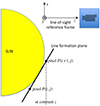 |
Fig. 1.
|

In Appendix A, we derive the expressions of div H, JZ and Jx, y as a function of the l.o.s. reference frame magnetic field coordinates, when the fields are measured along an inclined formation plane perpendicular to the local solar radius unit vector, R, of l.o.s. components Rx, y, z given in Eq. (1). We obtain
 (9)
(9)
We use H(m) to denote the vector measured along the inclined plane, where the line is formed. Oxyz is the l.o.s. reference frame and Oy is solar north oriented. Also,  and
and  are the difference of the measured component,
  or
or  , respectively, between two neighboring pixels in x or y direction. Then, Δx or Δy denotes the distance between the neighboring pixels in the “sky plane”, which is the plane perpendicular to the l.o.s. at the location of the observed region. The magnetic field may eventually be averaged between the two lines. If this average has to be performed before the ambiguity is solved, the acute angle method is applied between the two lines to select the ambiguous solutions to average. This is a reasonable approximation, which saves computation time in the simulated annealing. This corresponds to assume that the field lines do not twist so much. As for
  , it is the difference between the values obtained from the two lines with a difference in depth formation Δz along the l.o.s. Explicit definitions of all these quantities are given in Appendix A. The way to calculate these quantities is detailed at the beginning of the Appendix. When the map center is located on the solar equator and when b0 = 0, the above Eq. (9) is simplified to
 (10)
(10)
where θ is the heliocentric angle (positive for the western side of the central meridian and negative for the eastern side). The second line of these equations accounts for the z variation hidden in  and
and  , because H(m) is measured along the line formation plane, which is not perpendicular to Oz in the general case.
In other words, if we consider two neighboring pixels, referred to as P(i,j) and P(i+1,j), separated by the length Δx in the plane perpendicular to the line of sight, and if we also consider a quantity A measured via the same line at the two places (i.e., Ai, j and Ai + 1, j) the ratio (Ai + 1, j − Ai, j)/Δx = ΔxA/Δx is not an approximate value of the partial derivative ∂A/∂x. This is because ΔxA also involves a variation along the line of sight z together with the variation in x, when the observation is not performed at the disk center; namely, when the line formation plane is not perpendicular to the line of sight. From the definition, ∂A/∂x has to be evaluated at constant y and z. In the evaluation of ΔxA = Ai + 1, j − Ai, j, we have z[P(i+1,j)] ≠ z[P(i,j)], as it is visible in Fig. 1, when the line formation plane is inclined with respect to the line of sight, which is also the Oz axis. As a consequence, z is not kept constant in the partial derivative numerical evaluation, when the observation is done out of disk center. This was the reason to perform the Appendix A calculations.
For the numerical computation, the divergence was computed at the center of a pixel, by averaging between the variations along each side of the pixel. We used two lines formed at two different depths. This gives us
 (11)
(11)
 (12)
(12)
 (13)
(13)
where the indexes (1) and (2) correspond to “line 1” and “line 2”.
For the current density vector component, JZ, along the direction perpendicular to the inclined plane, we obtain (curl of the magnetic field):
![Mathematical equation: $$ \begin{aligned} J_{Z} &=R_{z}\left[ \frac{\Delta _{x}H_{y}^{(m)}}{\Delta x}-\frac{ \Delta _{y}H_{x}^{(m)}}{\Delta y}\right]\nonumber \\&\quad +R_{x}\frac{\Delta _{y}H_{z}^{(m)}}{\Delta y}-R_{y}\frac{\Delta _{x}H_{z}^{(m)}}{\Delta x}\cdot \end{aligned} $$](/articles/aa/full_html/2025/02/aa48632-23/aa48632-23-eq22.gif) (14)
(14)
It is possible to obtain analogously the two components of the current density vector in the plane perpendicular to the line of sight (see Appendix A):
![Mathematical equation: $$ \begin{aligned} J_{x}&=\left[ \frac{\Delta _{y}H_{z}^{(m)}}{\Delta y}-\frac{\Delta _{z}H_{y}^{(m)}}{\Delta z}\right] +\frac{R_{y}}{R_{z}}\frac{\Delta _{z}H_{z}^{(m)}}{\Delta z},\end{aligned} $$](/articles/aa/full_html/2025/02/aa48632-23/aa48632-23-eq23.gif) (15)
(15)
![Mathematical equation: $$ \begin{aligned} J_{y}&=\left[ \frac{\Delta _{z}H_{x}^{(m)}}{\Delta z}-\frac{\Delta _{x}H_{z}^{(m)}}{\Delta x}\right] -\frac{R_{x}}{R_{z}}\frac{\Delta _{z}H_{z}^{(m)}}{\Delta z}\cdot \end{aligned} $$](/articles/aa/full_html/2025/02/aa48632-23/aa48632-23-eq24.gif) (16)
(16)
From these relations and by applying Eq. (7), the z component of the current density vector in the line of sight reference frame can be derived, which is
 (17)
(17)
which can be reduced into
![Mathematical equation: $$ \begin{aligned} J_{z} &=\left[ \frac{\Delta _{x}H_{y}^{(m)}}{\Delta x}-\frac{\Delta _{y}H_{x}^{(m)}}{\Delta y}\right]\nonumber \\&\quad +\frac{R_{x}}{R_{z}}\frac{\Delta _{z}H_{y}^{(m)}}{\Delta z}-\frac{R_{y}}{ R_{z}}\frac{\Delta _{z}H_{x}^{(m)}}{\Delta z}\cdot \end{aligned} $$](/articles/aa/full_html/2025/02/aa48632-23/aa48632-23-eq26.gif) (18)
(18)
The second line of the formula accounts for the inclination of the line formation plane with respect to the line of sight. Then, JX and JY can be derived by applying Eq. (7) to Jx, Jy, and Jz.
In the following, we have plotted the heliographic reference frame components, JX, Y, Z, of the current density vector. For our plots, we derived the current density vector coordinates in the heliographic reference frame from the magnetic field unique vector (after disambiguation) rotated into the heliographic reference frame by applying Eq. (7).
Crouch et al. (2009) and Crouch (2013, 2015) developed a different calculation for also accounting for the departure from disk center, which implies that the line of sight is not perpendicular to the line formation plane. They also obtained that additional terms have to be introduced into the usual divergence expression. However, their formula given in Eqs. (4)–(5) of Crouch et al. (2009) and Crouch (2013, 2015) is different from our Eq. (9) because the corresponding reference frames are not the same. The divergence applied in Crouch et al. (2009) and Crouch (2013, 2015) uses spatial derivatives with respect to the heliographic X and Y and line of sight z coordinates, which do not form a rectangular reference frame; whereas our divergence uses spatial derivatives with respect to all the line of sight (x, y, z) reference frame coordinates. Our approach takes into consideration the fact that the observed lines are formed along inclined planes. Both approaches are different ways to treat the problem of the inclined line of sight.
4.4. The two-line formation depth difference
The quantity to be determined is the difference in the line of sight formation depth between the two lines. As it can be seen in Fig. 4 of Khomenko & Collados (2007), the two lines Fe I 6302.5 Å and 6301.5 Å are particularly interesting because their formation depths exhibit a strikingly parallel behavior. As also visible in Fig. 4 of Khomenko & Collados (2007), such a parallelism is not the case for the pair of Fe I 6302.5 and 5250.2 lines. This was the reason we discarded 5250.2, even though it is more sensitive to the magnetic field than 6301.5. Such a parallelism probably originates from the fact that the two lines 6302.5 and 6301.5 belong to the same multiplet n. 816 and have different gf values; these are, respectively, gf = 0.180 for 6301.5 and gf = 0.0627 for 6302.5 from the Kurucz data-basis. Since differential non-LTE effects within multiplets are thought to be very small, as proven by detailed, multi-level, non-LTE computations, this implies that the absorption coefficient of 6301.5 is three times larger than the absorption coefficient of 6302.5. There is then no doubt that 6301.5 forms higher than 6302.5. In other words, the optical depth of 6301.5 is almost 3, where the optical depth of 6302.5 is unity.
The two-iron-line formation difference in the quiet sun atmosphere was recently determined by a phase-shift analysis of HINODE observations by Faurobert et al. (2009). These authors obtained the observed value 63.2 ± 0.9 km, which is corroborated by the value of 69 km derived by the same phase-shift technique applied to theoretical profiles computed with the non-LTE Uitenbroek’s code (Grec et al. 2010).
However, it has to be remarked that the formation height varies along the line profile. The highest value, which is typically several hundreds of km, is reached at line center; whereas in the far wings, the formation height is nearly 0 km in the visible range. However, in the inversion algorithm, the mean squared difference between observed and theoretical profiles is computed over the whole profile. As the Zeeman effect is maximum around line center, this part of the profile is the most contributing to the field vector determination, so it it is quite natural to assign the line center formation height to this field value. For instance, it has been found that the value of 1/2arctanU/Q computed at the line center provides the field azimuth within a very good first approximation.
In addition, it has to be remarked that the formation depth has a certain thickness, which is aptly represented by the behavior of the contribution function. We have plotted the contribution functions in Fig. 2 at line center for the two iron lines. This figure has been obtained by applying a non-LTE polarized radiation transfer code (Landi Degl’Innocenti et al. 1990; Bommier et al. 1991) to the Fe I 6302.5 and 6301.5 line formation in the quiet sun reference model atmosphere of Maltby et al. (1986) and in the absence of a magnetic field. It can be seen in the figure that the formation depth of each line is characterized by a level of accuracy that is on the order of ±75 km, which is the halfwidth of the contribution function. However, the difference Δz = 66 km between the two lines remains clearly visible all along the profile of the contribution function. In Fig. 2, we have also indicated with arrows the height of τ = 1, which we consider as the line formation depth following the Eddington-Barbier approximation. It is well visible that this height correctly represents the mean line formation depth. In Fig. 4 of Khomenko & Collados (2007), we can also see that the formation depth difference remains on the order of Δz = 70 km in the quiet sun, whatever the actual formation depth is.
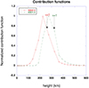 |
Fig. 2. Contribution functions of the two lines Fe I 6302.5 Å and 6301.5 Å as a function of the height above τ5000 = 1. The heights where τ = 1, which is the line formation height in the Eddington-Barbier approximation, are indicated by arrows. |
Finally, in Fig. 4 of Khomenko & Collados (2007), we can observe that the depth difference is larger in active regions than in quiet ones. We thus applied instead the depth difference of 98 km at the disk center for active regions. This is also the value determined with the non-LTE Uitenbroek’s code (Grec et al. 2010) in a previous approximation.
Finally, we derived the line formation depths from a model that we describe below. The temperature, electron pressure, and gas pressure were first taken from an atmospheric model. We used the Maltby et al. (1986) quiet sun photospheric reference model extrapolated downwards beyond −70 km to −450 km below the τ5000 = 1 level (courtesy of Instituto de Astrofísica de Canarias (IAC)). The continuum absorption coefficient was evaluated according to the MagnetoActive Fraunhofer LInes Stokes Parameters Profiles (MALIP) code of Landi Degl’Innocenti (1976). This was done, in particular, by including H− bound-free, H− free-free, neutral hydrogen atom opacity, Rayleigh scattering on H atoms, and Thompson scattering on free electrons. The line absorption coefficient was derived from the Boltzmann and Saha equilibrium laws, taking the two first ions of element into account. The atomic data were taken from Wiese or Moore and the partition functions from Wittmann. The iron abundance was assumed to be 7.60 and the sodium abundance 6.25 in the usual logarithmic scale, where the abundance of hydrogen is 12. A depth-independent microturbulent velocity field of 1 km/s was introduced. Finally, departures from LTE in the ionization equilibrium were simulated for layers above τ5000 = 0.1 by applying Saha’s law with a constant radiation temperature of 5100 K, instead of the electron temperature provided by the atmospheric model.
At final step, the line center optical depth grid was scaled to the continuum optical depth grid by applying the respective absorption coefficients. We used the continuum optical depth grid provided in the atmospheric model and the transfer equation was not explicitly solved again. The height of formation of the line center was then determined as follows. Once obtained the grid of line center optical depths, the height of formation of the line center was located where the optical depth along the line of sight is unity (Eddington-Barbier approximation); namely, where τ/μ = 1 and τ is the line center’s optical depth along the vertical and μ is the cosine of the heliocentric angle θ (here supposed to be 0). As seen in Fig. 5 of Bruls et al. (1991) and in Fig. 2 of the present paper, this conveniently represents the depth where the contribution function has its maximum.
We thus obtained quiet sun line center formation heights of 262 km for Fe I 6302.5 and 328 km for Fe I 6301.5 above the τ5000 = 1 level. This leads to a difference of 66 km in excellent agreement with the measurements described above, which validates our computation method.
4.5. The aspect ratio of the strongly stratified atmosphere
We were indeed confronted with the problem that the vertical gradient of the magnetic field, μ0∂Hz/∂z, was found to be on the order of 3 G/km in the spot umbrae, whereas the horizontal gradient μ0∂Hx/∂x + μ0∂Hy/∂y was only on the order of 0.3 G/km. This leads to a non-vanishing value of div H, whatever the signs would be. We then investigated the literature and found 15 references, which fully confirm these values provided by different instruments (ground-based as well as spaceborne), different inversion methods (SIR or others), and different spectral lines. The detailed description of these references can be found in Bommier (2013). An observation review was also presented by Balthasar (2018). All concluded to the above cited values. In other words, a loss of magnetic flux is observed with increasing height, which is not compensated for by an increase of the horizontal flux. In Bommier (2013, 2014), we showed that the lack of spatial resolution in both transverse and along the line of sight directions cannot be held responsible for the seemingly non-vanishing observed div H. This was based on mathematical study of the convolution procedure. It was shown that the divergence computed with averaged quantities is equal to the average of the local divergences. Accordingly, if the local divergence is zero, the divergence computed with averaged quantities should also be zero, within the noise level. The question arised to know if the observed value of div H is an effect of different spatial resolution along the different space directions. The effect of the spatial resolution (horizontal as well as vertical) is filtering. The mathematical demonstration that the filtered divergence is the divergence of the filtered quantity is given in Bommier (2013, 2014). Bommier (2014) included also a more straightforward demonstration in the spatial Fourier space. The same demonstration applies to the spatial averaging and the effect of the magnetic filling factor α. As explained in the previous section, we only know the “local average magnetic field”, αH, from the measurements, but the average divergence is the divergence of the averaged field. In addition, Bommier (2014) provides results of numerical tests devoted to investigate an eventual effect of the limited spatial resolution (eventually anisotropic). The numerical tests are all negative. They conclude with a zero divergence computed by finite differences, when the local divergence is zero. In our opinion, the negation of this logical proposition is that the non-zero observed value for the divergence indicates a non-zero local value. In Bommier (2015), we present a discussion about the necessity for div H to be zero. We argue that the existence of magnetic monopoles is not the only possibility for a non-zero div H. Following a discussion about the measurement noise level effect, we present below another possibility we have investigated.
In the THÉMIS measurements described in Bommier et al. (2007), which is the validation paper of the UNNOFIT inversion method, the polarimetric noise is assumed to be 1.5 × 10⁻³. As reported in Sect. 2, this results in an inaccuracy of 10 G for the longitudinal field and 15 G for the transverse field. The field difference observed between and from the two line 6301.5 and 6302.5 is about 300 G, when the difference in line formation height is about 100 km, close to the disk center. This results in an inaccuracy of 0.2 G/km for the vertical field gradient observed at the disk center. As for the transverse field, the typical THÉMIS pixel size is about 500 km (Bommier 2013), which results in an inaccuracy of less than 0.2 G/km for the horizontal field gradient observed at the disk center. The total inaccuracy on the observed div H value results in 0.4 G/km, to be compared to the non-vanishing value of 2.7 G/km, which results from the measurements reported in the literature. The non-vanishing value observed for div H is then markedly higher than the noise level.
We then investigated how the magnetic field is influenced by the plasma anisotropy due to the strong stratification due to the gravity and the density at the star surface, which is responsible for an “aspect ratio” between horizontal and vertical typical lengths, respectively denoted as lh and lv. In the case of the solar photosphere, by applying strongly stratified fluid mechanics laws following Brethouwer et al. (2007), we evaluated this aspect ratio to be on the order of lh/lv = 20 (Bommier 2013, 2014) in the quiet sun photosphere. In Bommier (2020), we showed that what is measured by Zeeman effect is the magnetic field H and not the magnetic induction B. The magnetic induction B is divergence-free, which implies that div H = −div M, where M is the magnetization. The magnetization is linked to the matter. Accordingly, it scales following the typical lengths introduced above. It reveals that once the inverse of the aspect ratio is applied to scale the different magnetic field components, the scaled div H vanishes, which enables the ambiguity resolution that we report in this paper. An example of this result in the case of NOAA 10808 observed with THÉMIS on September 13, 2005 is shown in Fig. 3 of Bommier (2013). Although we evaluated the theoretical value of the aspect ratio on the order of 20 in the quiet sun photosphere, this ratio may eventually be different in sunpots or plages or active regions, as in the case of the regions we treated. This is not so widely known and sometimes we continued to adjust the ratio (kept constant in the whole map) until the ambiguity resolution was consistent across the whole map. Here, the word “consistent” is meant to indicate that the resulting map does not show any artificial strong current line, which would delineate sharp azimuth change due to ambiguous solution selection change. The resulting map displays (at most) homogeneous field directions. We obtain that this inverse scaling is a necessity for a correct ambiguity resolution. The correctness is obtained by comparison with the intuitive ambiguity solution, which can be found in sunpot penumbrae as discussed in the following subsection. We applied the Maxwell law curl H = J for the current density derivation from the magnetic field vector in different regions reported in the following subsections.
4.6. Verification of the ambiguity resolution results
In this way, we treated 60 maps observed in Fe I 6301/6302 and 26 maps observed in Na I D with THÉMIS (in 2010–2013) and 23 HINODE/SOT/SP observations of active regions2. For the sunspots the correctness of the solution can be verified because the spot umbra polarity is known from circular polarization. This is true even near the limb, where the solar vertical field at spot center is nearly transverse with respect to the l.o.s. The ambiguity solution is good if it is in agreement with the polarity. It has to be remarked that for a sunspot observed anywhere on the disk there is always a place in it where the ambiguity solution can be derived from the spot polarity. This place is either in the penumbra, when the spot is observed near the disk center, or in the umbra, when the spot is observed near the limb. We consider such cases to be possibilities of observational proofs of our disambiguation method and we obtained successful proofs even in a spot at μ = 0.42, which is θ = 65° from the disk center.
4.7. Test of the method on theoretical data
Our method for taking the departure from disk center into account, which leads to additional terms in the divergence formula Eq. (9), has been tested on theoretical data. Divergence-free data were prepared by simulating two close sunspots forming a δ-spot and by applying the magnetic field model described by Eqs. (8)–(10) of Fan & Gibson (2004). Simulation results based on this model have been used to study δ-spots (as in Fig. 3 of Leka et al. 2005) and also to test various ambiguity resolution methods, as in Metcalf et al. (2006). The ambiguity of the transverse magnetic field in the line of sight reference frame was simulated and submitted to the ME0 ambiguity resolution code of Leka et al. (2009), which was modified by us for taking the vertical magnetic field gradient ∂Hz/∂z from two-line observations instead from extrapolation as described at the beginning of Sect. 4. The two-line observation had been simulated with theoretical results at two different depths separated by 70 km along the line of sight. The pixel sizes were assumed to be Δx = 1160 km and Δy = 581 km, as in our THÉMIS observations described in Bommier (2013). The δ-spot was assumed to be far from disk center and located at 30° from the central meridian in longitude and at 45° in latitude. The solar disk center latitude was assumed to be zero.
Performance metrics for the limited resolution case for our DIVB resolution algorithm applied to the test data of Leka et al. (2009) and Crouch (2013).
The test result is represented in Fig. 3, where the theoretical reference field is plotted in the top map. The result of the disambiguation when the usual divergence formula is applied, which is given by the first line of Eq. (9) only, is displayed in the middle map. The minimized quantity is in fact |div H| + λ|JZ| with λ = 1 as in our method. It can be seen that the amiguity resolution widely fails over the δ-spot. When the full Eq. (9) is applied instead, the obtained result is displayed in the bottom map of Fig. 3, which is in total agreement with the reference field. Thus, we confirm via numerical test that the second line of Eq. (9) is necessary to resolve the ambiguity by applying a two-line analysis to maps observed out of disk center as discussed after Eq. (10) and in Fig. 1.
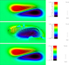 |
Fig. 3. Result of the ambiguity resolution test using our method applied to theoretical data. Top: Map of the input magnetic field vector. Middle: ambiguity resolution by applying the usual divergence formula (first line of Eq. (9) only) to these data, where the region is assumed to be out of disk center and where two lines formed at two different altitudes are supposed to be observed. Bottom: Ambiguity resolution by applying Eq. (9). |
4.8. Test of the resolution code on theoretical data
We tested our ambiguity resolution code DIVB2 (for: divergence of B) built on the method described above on the theoretical test data described in Leka et al. (2009). These data were used for testing various ambiguity resolution methods as in Leka et al. (2009). The methods by Crouch et al. (2009) and Crouch (2013, 2015) also used magnetic field data at two different heights, which were applied to the current test data. We used two series of these data.
The first series was the “flower” data, where the sunspots are simulated with form of flowers, as visible in Fig. 4 of Leka et al. (2009). These data were prepared to test the code robustness against lack of spatial resolution. The preparation of the theoretical data is described on p. 93 of Leka et al. (2009) and also on p. 111 of Crouch (2013). We used the theoretical data with averaged pixel sizes of 0.3″ and 0.9″. These theoretical data are provided at two heights separated by 0.18″. These data simulate location at the disk center, namely, the line of sight is assumed to be perpendicular to the line formation planes. For these data, we obtained the result metrics listed in Table 1. The metrics is given by the fraction of pixels with correct ambiguity resolution in the whole map, ℳarea, and the fraction of pixels with correct ambiguity resolution within the conditions of transverse field H⊥ stronger than 100 G and 500 G, respectively. As seen in Table 1, our code obtains excellent results for the two resolution cases.
The second series of data was the simulation represented in Fig. 1 of Leka et al. (2009). These data were artificially noised by adding them a theoretical photon noise, at the level of polarimetric accuracy of 10−3 for the low noise case and 10−2 for the high noise case, as described on p. 89 of Leka et al. (2009). The assumed pixel size was 0.5″. The case without any added noise was also treated. These data are available at two heights. We used data at two heights distant of 890 km along the l.o.s., whereas Crouch (2013) used data at two heights distant of the pixel size as described in p. 111 of Crouch (2013), which is 376 km only. For these data, we obtained the result metrics listed in Table 2. In this case also, our code obtains very good results. The results are perfect in the case without any noise. The highest noise level, which is 10−2 in polarization, is rather high and higher than the current observation polarization inaccuracies. In the case of this high level noise, we obtain nevertheless rather good results better than 80% correct for the high noise level and better than 95% correct for the low noise level. As visible in Table 2, our worst results locate in weak magnetic field regions.
Performance metrics for the noise-added case for our DIVB resolution algorithm applied to the test data provided by K.D. Leka’s courtesy.
This second series of data were assumed to be located out of disk center at latitude 9° South and longitude 36° East with respect to the central meridian. This leads to an heliocentric angle cosine μ = cos θ = 0.80, which is rather far from disk center. It has to be remarked that we obtain perfect ambiguity resolution result with our code in the no noise case as visible in the first line of Table 2. In our code, the disambiguation is performed in the l.o.s. reference frame and we applied Eq. (9) to account for departure from disk center in the case of lines formed along horizontal planes, which is done in the second line of Eq. (9). The success of our resolution of theoretical data again validates our Eq. (9) and, in particular, its second line in the case of lines formed along horizontal planes and observed out of disk center.
5. Results: Examples of vector maps
The results presented below were obtained from 86 maps observed with THÉ MIS and 23 maps observed by HINODE/SOT/SP, which are visible in V. Bommier’s personal page3. The magnetic field final values are also available on-line there. Four examples of HINODE data and two examples of THÉMIS data are included in Figs. 4–9 below. For accuracy reasons, the HINODE data pixels were two times binned two by two before the ambiguity resolution, which results in pixel sizes of Δx = 862 km and Δy = 928 km. The THÉMIS data pixel size was Δx = 794 km and Δy = 725 km, the binning was not performed.
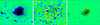 |
Fig. 4. Active region NOAA 11420 observed by HINODE/SOT/SP on February 18, 2012 between 11:08 and 12:04 UT. The ambiguity is resolved by our method. Left: Magnetic field vector, vertical component between −2040 and +2040, horizontal component maximum arrow length 1355 G. Middle: current density vector, vertical component between −64 and +64, horizontal component typical arrow length 5000 mA/m2. Right: Lorentz force vector, vertical component between −448 and +448, horizontal component typical arrow length 800 mN/m2. The spatial resolution was reduced by a factor 5 × 5 for paper file size purposes (color figure on-line). |
The plotted Lorentz force displays the correct direction of the force, but may not actually be the exact force strength. What is, in fact, plotted in the following figures is J × μ0H, when the Lorentz force is in fact J × B. The magnetic induction B, the magnetic field H and the magnetization M are all parallel, because
 (19)
(19)
where ne and ni are the electron and ion densities respectively, kB is the Boltzmann constant, and T is the temperature (Delcroix & Bers 1994). The minus sign implies that M is antiparallel to B, which is plasma diamagnetism. This can be also written as
 (20)
(20)
where βc is the plasma β, ratio of kinetic energy to magnetic energy, however, this is expressed in terms of the charged particle density
 (21)
(21)
In the usual photospheric electron and ion densities, μ0M remains negligible with respect to μ0H and B, which are then equal, and the following figures would display the full Lorentz force. However, if the electron density is higher, following the suggestion of interior electron thermal escape by Bommier (2020), μ0M can become non-negligible, so that the length of the Lorentz force vectors would not be exact in the following figures, even if the vector direction is correct.
5.1. HINODE data: Examples of a single regular spot
We systematically observe a strong circular horizontal current component, which wraps spots clockwise about a positive polarity spot and counterclockwise about a negative polarity spot. As a consequence, the Lorentz force vector is systematically found centripetal with respect to the spot center. Numerous examples can be found along the web page. We can cite in particular the active regions: NOAA 11420 observed by HINODE/SOT/SP on February 18, 2012 between 11:08 and 12:04 UT (negative polarity spot), which is represented in Fig. 4, and NOAA 11494 observed by HINODE/SOT/SP on June 7, 2012 between 14:15 and 15:05 UT (positive polarity spot), which is represented in Fig. 5. These examples can be found in the web page with a better spatial resolution. Similar examples can be found in the web page for HINODE/SOT/SP observations of single spots on December 12, 2006, September 7, 2011, February 1, 2012, May 1, 2012, and June 13, 2012.
 |
Fig. 5. Active region NOAA 11494 observed by HINODE/SOT/SP on June 7, 2012 between 14:15 and 15:05 UT. The ambiguity is resolved by our method. Left: magnetic field vector, vertical component between −2150 and +2150, horizontal component maximum arrow length 1743 G. Middle: Current density vector, vertical component between −219 and +219, horizontal component typical arrow length 5000 mA/m2. Right: Lorentz force vector, vertical component between −682 and +682, horizontal component typical arrow length 800 mN/m2. The spatial resolution was reduced by a factor 5 × 5 for paper file size purposes (color figure on-line). |
5.2. HINODE data: Examples of a neutral line
We often observe a strong horizontal current component, which crosses the neutral line. Two examples are presented in this paper, which can also be found in the web page: NOAA 11476 observed by HINODE/SOT/SP on May 12, 2012 between 02:38 and 03:11 UT, which is represented in Fig. 6, and NOAA 11429 observed by HINODE/SOT/SP on March 6, 2012 between 22:10 and 22:43, which is represented in Fig. 7. We can refer to the web page for a better spatial resolution. NOAA 11476, which is represented in Fig. 6, produced numerous C-class flares and NOAA 11429, which is represented in Fig. 7, produced an X-class flare followed by a CME. The example of September 7, 2011, which is visible in the web page, is also the case of an active region that produced an X-class flare. A strong horizontal current component is well visible across the neutral line.
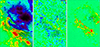 |
Fig. 6. Active region NOAA 11476 observed by HINODE/SOT/SP on May 12, 2012 between 02:38 and 03:11 UT. The ambiguity is resolved by our method. Left: Magnetic field vector, vertical component between −2450 and +2450, horizontal component maximum arrow length 2470 G. Middle: current density vector, vertical component between −218 and +218, and horizontal component typical arrow length 8000 mA/m2. Right: Lorentz force vector, vertical component between −1040 and +1040, and horizontal component typical arrow length 800 mN/m2. The spatial resolution was reduced by a factor 5 × 5 for paper file size purposes (color figure online). |
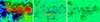 |
Fig. 7. Active region NOAA 11429 observed by HINODE/SOT/SP on March 6, 2012 between 22:10 and 22:43 UT. The ambiguity is resolved by our method. Left: Magnetic field vector, vertical component between −2480 and +2480, horizontal component maximum arrow length 2441 G. Middle: Current density vector, vertical component between −185 and +185, horizontal component typical arrow length 5000 mA/m2. Right: Lorentz force vector, vertical component between −1180 and +1180, and horizontal component typical arrow length 800 mN/m2. The spatial resolution was reduced by a factor 5 × 5 for paper file size purposes (color figure online). |
5.3. THÉMIS data: Example of a single regular spot
The example presented in this paper is the case of NOAA 11857 observed with THÉMIS on October 7, 2013, between 08:57 and 09:22 UT in Fe I 6301/6302. In the case of the photosphere, which is observed in Fe I 6301/6302 and represented in Fig. 8, we find again the current and Lorentz force characteristics described above; namely, circular current about the spot and centripetal Lorentz force. NOAA 11857 was observed with THÉ MIS on October 5, October 7 (two times, morning and afternoon), October 8, and October 9. All these examples are visible in the web page. The magnetic field is more rotating about the spot center at the chromospheric level than at the photospheric level, where it is more radial.
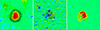 |
Fig. 8. Active region NOAA 11857 observed with THEMIS on October 7, 2013 between 08:57 and 09:22 UT, in the photospheric lines Fe I 6301/6302. The ambiguity is resolved by our method. Left: Magnetic field vector, vertical component between −1790 and +1790, and horizontal component maximum arrow length 1070 G. Middle: Current density vector, vertical component between −68 and +68, and horizontal component maximum arrow length 746 mA/m2. Right: Lorentz force vector, vertical component between −56 and +56, and horizontal component maximum arrow length 133 mN/m2 (color figure online). |
5.4. THÉMIS data: Example of a neutral line
The example presented in this paper is the case of NOAA 11865 observed with THÉMIS on October 11, 2013, between 09:39 and 09:59 UT in Fe I 6301/6302. Again, in the photosphere, which is represented in Fig. 9, we observe a strong horizontal current component across the neutral line.
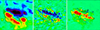 |
Fig. 9. Active region NOAA 11865 observed with THEMIS on October 11, 2013 between 09:39 and 09:59 UT, in the photospheric lines Fe I 6301/6302. The ambiguity is resolved by our method. Left: Magnetic field vector, vertical component between −1450 and +1450, and horizontal component maximum arrow length 1320 G. Middle: Current density vector, vertical component between −96 and +96, and horizontal component maximum arrow length 655 mA/m2. Right: Lorentz force vector, vertical component between −83 and +83, and horizontal component maximum arrow length 43 mN/m2 (color figure on-line). |
6. Conclusion
We have shown that observations in two different lines, which belong to the same multiplet but have different absorption coefficients and thus formed at two different depths (e.g., Fe I 6302.5 Å and 6301.5 Å) enable the resolution of the azimuth ambiguity that is left over from the Zeeman signal interpretation. The anisotropy of the strongly stratified plasma of the photosphere has also to be accounted for following Bommier (2013, 2014). As a consequence, two ambiguity-resolved field vector maps are obtained at two different but close altitudes, which enable the derivation of the current density full vector via curl H = J. This reveals the horizontal component of the current density, which is found markedly stronger than the better known vertical one, as already observed by Puschmann et al. (2010a) from HINODE/SOT/SP data. We observe some systematical trends, such as circular currents wrapping spots clockwise about a positive polarity spot and counterclockwise about a negative polarity spot and strong horizontal current components, which cross active region neutral lines. The wrapping direction with respect to the spot polarity is the same as the average one in Fig. 1 of Puschmann et al. (2010a), where completely different methods were used. As a result, the Lorentz force may be computed. It is found to be centripetal in sunspots. The sunspots are thus maintained by the force.
We found that the anisotropic scaling of the real solar data following the aspect ratio in the strongly stratified medium of the solar photosphere, suggested by Bommier (2013, 2014), has to be applied for a correct resolution of the ambiguity. The correctness can be established by comparison with the intuitive ambiguity solution, which can be derived in spot penumbrae from the spot polarity. The necessity of applying the aspect ratio for solving the ambiguity is another main result of the present work.
This can be done by applying an anisotropic scaling factor to the data before disambiguation. For instance, by artificially dividing by 10 the pixel sizes before submission to the Azimuthal Ambiguity Resolution (AMBIG2) code proposed by Crouch (2013) for two lines. This code also requires that the observed region be located close to disk center. Our disambiguation code is able to also disambiguate data of regions located out of the disk center.
Finally, we can remark that the Na I D1 and D2 lines form another favorable line pair, because they are also two lines of the same multiplet, but with different absorption coefficients. We evaluated their quiet sun line center formation heights at 533 km for Na I D1 and 604 km for Na I D2 above the τ5000 = 1 level. These lines are then located in the low chromosphere close to the temperature minimum and with a difference of 71 km. Observing this line pair would open access to the low chromosphere where they are formed. However, a better spatial resolution for both observations and analysis would probably be necessary in such a medium.
In the present analysis, the spatial resolution of both observations and analysis is very limited. The Stokes inversion was performed with average over the whole observed pixel. The presence of unresolved magnetic fields was however roughly accounted for by means of a magnetic filling factor α, which was introduced and determined in the inversion. However, active regions such as those studied here, which include sunspot umbræ and penumbræ, have a structure akin to dots that are smaller than the present pixel sizes. This concerns the horizontal spatial resolution, but the vertical spatial resolution of our study is limited also, because it is limited to the difference in line formation depth of two lines, which is found not so far from the vertical height scale. As a rough first approach, we assume a constant formation depth difference for the two lines under interest, although our images include various different structures, where this difference may vary. A better vertical spatial resolution would be attained by applying for instance the SIR inversion code (Ruiz Cobo & del Toro Iniesta 1992).
A series of other effects able to perturb the sunspot magnetic field measurements is detailed in the above Sect. 3, including: velocity or magnetic field-temperature correlations, blending by molecular lines, straylight from penumbra, departure from a purely hydrostatic equilibrium, non-horizontal and corrugated τ = 1 surface, and non-LTE effects in spectral lines. Consequently, as long as these and other effects have not been properly tested in realistic model atmospheres and with state-of-the-art radiative transfer computations, the scaling factor we introduce must be taken as a purely empirical factor.
Acknowledgments
The author is grateful to an anonymous referee for refined suggestions, reported in this paper. Some reported observations were made with the French-Italian telescope THÉMIS operated by the CNRS on the island of Tenerife in the Spanish Observatorio del Teide of the Instituto de Astrof ísica de Canarias. We are grateful to B. Lites for the level-1 HINODE/SOT/SP data. For the data inversion, this work was granted access to the HPC resources of MesoPSL financed by the Region Ile de France and the project Equip@Meso (reference ANR-10-EQPX-29-01) of the Investissements d’Avenir program supervised by the Agence Nationale pour la Recherche.
References
- Balthasar, H. 2018, Sol. Phys., 293, 120 [NASA ADS] [CrossRef] [Google Scholar]
- Bommier, V. 2013, Phys. Res. Int., 2013, 195403 [NASA ADS] [CrossRef] [Google Scholar]
- Bommier, V. 2014, C.R. Phys., 15, 430 [NASA ADS] [CrossRef] [Google Scholar]
- Bommier, V. 2015, in IAU Symposium, eds. K. N. Nagendra, S. Bagnulo, R. Centeno, & M. Jesús Martínez González, Polarimetry, 305, 28 [NASA ADS] [Google Scholar]
- Bommier, V. 2020, A&A, 634, A40 [NASA ADS] [CrossRef] [EDP Sciences] [Google Scholar]
- Bommier, V., Landi Degl’Innocenti, E., & Sahal-Bréchot, S. 1991, A&A, 244, 383 [NASA ADS] [Google Scholar]
- Bommier, V., Landi Degl’Innocenti, E., Landolfi, M., & Molodij, G. 2007, A&A, 464, 323 [NASA ADS] [CrossRef] [EDP Sciences] [Google Scholar]
- Brethouwer, G., Billant, P., Lindborg, E., & Chomaz, J. M. 2007, J. Fluid Mech., 585, 343 [NASA ADS] [CrossRef] [Google Scholar]
- Bruls, J. H. M. J., Lites, B. W., & Murphy, G. A. 1991, in Solar Polarimetry, Proceedings of the 11st National Solar Observatory/Sacramento Peak Summer Workshop, Sunspot, New Mexico, 27-31 August 1990, ed. L. J. November (National Solar Observatory), 444 [Google Scholar]
- Buehler, D., Lagg, A., Solanki, S. K., & van Noort, M. 2015, A&A, 576, A27 [NASA ADS] [CrossRef] [EDP Sciences] [Google Scholar]
- Crouch, A. D. 2013, Sol. Phys., 282, 107 [NASA ADS] [CrossRef] [Google Scholar]
- Crouch, A. D. 2015, Sol. Phys., 290, 2677 [NASA ADS] [CrossRef] [Google Scholar]
- Crouch, A. D., Barnes, G., & Leka, K. D. 2009, Sol. Phys., 260, 271 [NASA ADS] [CrossRef] [Google Scholar]
- Delcroix, J. L., & Bers, A. 1994, Physique des Plasmas (7, rue de l’Estrapade, 75005 Paris: InterÉditions/CNRS Éditions) [Google Scholar]
- Fan, Y., & Gibson, S. E. 2004, ApJ, 609, 1123 [NASA ADS] [CrossRef] [Google Scholar]
- Faurobert, M., Aime, C., Périni, C., et al. 2009, A&A, 507, L29 [NASA ADS] [CrossRef] [EDP Sciences] [Google Scholar]
- Frutiger, C., Solanki, S. K., Fligge, M., & Bruls, J. H. M. J. 2000, A&A, 358, 1109 [NASA ADS] [Google Scholar]
- Gary, G. A., & Hagyard, M. J. 1990, Sol. Phys., 126, 21 [Google Scholar]
- Grec, C., Uitenbroek, H., Faurobert, M., & Aime, C. 2010, A&A, 514, A91 [EDP Sciences] [Google Scholar]
- Khomenko, E., & Collados, M. 2007, ApJ, 659, 1726 [Google Scholar]
- Landi Degl’Innocenti, E. 1976, A&AS, 25, 379 [NASA ADS] [Google Scholar]
- Landi Degl’Innocenti, E., Bommier, V., & Sahal-Bréchot, S. 1990, A&A, 235, 459 [Google Scholar]
- Landolfi, M., & Landi Degl’Innocenti, E. 1982, Sol. Phys., 78, 355 [NASA ADS] [CrossRef] [Google Scholar]
- Landolfi, M., Landi Degl’Innocenti, E., & Arena, P. 1984, Sol. Phys., 93, 269 [NASA ADS] [CrossRef] [Google Scholar]
- Leka, K. D., Fan, Y., & Barnes, G. 2005, ApJ, 626, 1091 [NASA ADS] [CrossRef] [Google Scholar]
- Leka, K. D., Barnes, G., Crouch, A. D., et al. 2009, Sol. Phys., 260, 83 [Google Scholar]
- Leka, K. D., Wagner, E. L., Griñón-Marín, A. B., Bommier, V., & Higgins, R. E. L. 2022, Sol. Phys., 297, 121 [NASA ADS] [CrossRef] [Google Scholar]
- Maltby, P., Avrett, E. H., Carlsson, M., et al. 1986, ApJ, 306, 284 [Google Scholar]
- Metcalf, T. R. 1994, Sol. Phys., 155, 235 [Google Scholar]
- Metcalf, T. R., Leka, K. D., Barnes, G., et al. 2006, Sol. Phys., 237, 267 [Google Scholar]
- Molodij, G., Bommier, V., & Rayrole, J. 2011, A&A, 531, A139 [NASA ADS] [CrossRef] [EDP Sciences] [Google Scholar]
- Puschmann, K. G., Ruiz Cobo, B., & Martínez Pillet, V. 2010a, ApJ, 721, L58 [Google Scholar]
- Puschmann, K. G., Ruiz Cobo, B., & Martínez Pillet, V. 2010b, ApJ, 720, 1417 [Google Scholar]
- Ruiz Cobo, B., & del Toro Iniesta, J. C. 1992, ApJ, 398, 375 [Google Scholar]
- Socas-Navarro, H. 2005, ApJ, 633, L57 [Google Scholar]
- Stenflo, J. O. 1973, Sol. Phys., 32, 41 [NASA ADS] [CrossRef] [Google Scholar]
- Vernazza, J. E., Avrett, E. H., & Loeser, R. 1973, ApJ, 184, 605 [NASA ADS] [CrossRef] [Google Scholar]
Appendix A: Expressions of the divergence and curl when the quantities are measured along an inclined line formation plane
We describe below how divergence and curl have to be computed, when the measurements are made in pixels, and when the spectral line used for the measurements is formed at a certain depth in the stellar atmosphere. This depth defines a formation plane for the line. In the following we neglect an eventual thickness of this plane, which we consider as infinitely sharp. We consider the general case where this plane is inclined with respect to the line of sight for an observation performed out of disk center. The case of disk center observation is however possible as a particular case.
We denote the heliographic reference frame as OXYZ and the l.o.s. reference frame as Oxyz with Oy solar north oriented. The point O where divergence and curl are computed is taken at longitude-latitude (L, b). The solar radius unit vector, R, in O is perpendicular to the the line formation plane, which is tangent to the solar surface. The R coordinates in the l.o.s. reference frame are given in Eq. (1). In the l.o.s. reference frame, the line formation plane, which is perpendicular to R of coordinates (Rx, Ry, Rz), has then for general equation
 (A.1)
(A.1)
We use H(1) to denote the magnetic field vector measured as a function of x and y along the formation plane of the line number (1). H(1) depends on the following variables
 (A.2)
(A.2)
where the semicolon means “such as”. A similar law holds for the magnetic field vector H(2) measured with the second line number (2). In the l.o.s. reference frame Oxyz, we denote as Δx and Δy the distance between two neighboring pixels along the Ox and Oy axes respectively in the “sky plane”. Let’s denote as  the variation of
  between two neighboring pixels in x direction (i + 1, j) and (i, j) distant of Δx in the image
 (A.3)
(A.3)
and analogously
 (A.4)
(A.4)
For the second line one can similarly define  and
and  . The magnetic field may be averaged between the two lines, with the acute angle method when the ambiguity is not resolved, and in this case we denote the average as
  and
and  . As for the z variation, it involves the two lines as
 (A.5)
(A.5)
A.1. Calculation of the divergence
The mathematical expression of div H is frame-independent
 (A.6)
(A.6)
However, a problem arises when it is discretized in the above described system of line formation planes.  , which could a priori be considered as the ∂Hx/∂x contribution, includes also a variation of
  along the Oz axis because the magnetic field is measured along the line formation plane. As a consequence,
  cannot finally be considered as an approximation of ∂Hx/∂x because ∂Hx/∂x is the variation of Hx with x at constant y and z following the mathematical definition.
This appendix is devoted to accounting for this difficulty by applying the Ostrogradski’s theorem, which is that the volume integrated divergence equals the flux of the quantity through the surface that borders the volume. We applied this theorem to the small volume delineated by four neighboring pixels separated by Δx and Δy in the sky plane xOy, but located in the line formation plane, and the corresponding four other pixels for the second line formed in another formation plane separated from the first one by the distance Δz along the line of sight. In the following, we detail three different derivations from the simplest to the most complex. We first consider an observation located at the solar equator without inclination of the solar rotation axis (Sect. A.1.1). We then generalize this demonstration to the general case (Sect. A.1.2) and we add a more elegant derivation leading to the same result as a third part (Sect. A.1.3).
A.1.1. Case of a region located at solar equator
We first assume that O is located on solar equator and that the Sun rotation axis lies in the plane of the sky, i.e. that b0 = 0. The heliocentric angle is denoted as θ. A section of the small volume introduced above is represented in Fig. A.1. For each side of the volume, a unit vector perpendicular to the surface and pointing towards the exterior of the volume can be plotted. Three of these vectors are plotted in Fig. A.1, S, S′, and S″. One has to calculate the flux of the magnetic field through each elementary surface. Consider first the surface element associated to the S vector. This surface element is part of the formation plane of line number (1), whereas S′ and S″ join the two line formation planes. In the l.o.s. reference frame Oxyz, the S unit vector has the following coordinates:
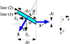 |
Fig. A.1. Reference frame for the divergence evaluation: case of an observation at the solar equator. The heliocentric θ angle is oriented by the Oy axis and is negative in the figure. The two formation planes corresponding to the two lines (1) and (2) are indicated by their respective number. The unit S vector is indeed the same as the unit R vector along the local solar radius. |
 (A.7)
(A.7)
As a consequence, the flux of the magnetic field through this surface per surface unit is
 (A.8)
(A.8)
As visible in Fig. A.1, the elementary surface value is ΔℓΔy, where
 (A.9)
(A.9)
The flux through this elementary surface is then finally
 (A.10)
The flux through the elementary surface associated to S′ is
 (A.11)
where the superscript (m) denotes the average between the two lines (1) and (2). Finally, the flux through the third elementary surface S″ is
 (A.12)
As the elementary volume is ΔℓΔyΔzcos θ = ΔxΔyΔz, one has finally in application of Ostrogradski’s theorem
![Mathematical equation: $$ \begin{aligned}&\mathrm{div}\boldsymbol{H}\ \Delta x\Delta y\Delta z \nonumber \\&= \left[ (H_{z}^{(1)}-H_{z}^{(2)})+(H_{x}^{(1)}-H_{x}^{(2)})\tan \theta \right] \ \Delta x\Delta y \\&+\left[ H_{x}^{(m)}(x+\Delta x,y)-H_{x}^{(m)}(x,y)\right] \ \Delta z\Delta y \nonumber \\&+\left[ H_{y}^{(m)}(x,y+\Delta y)-H_{y}^{(m)}(x,y)\right] \ \Delta x\Delta z\ , \nonumber \end{aligned} $$](/articles/aa/full_html/2025/02/aa48632-23/aa48632-23-eq75.gif) (A.13)
(A.13)
which results in Eq. (10) of the paper. The term in tanθ accounts for the line formation plane inclination with respect to the line of sight.
A.1.2. Generalization
One considers now a point O on the solar surface with longitude L and latitude b. The solar radius in O denoted as R is perpendicular to the line formation plane. The R coordinates in terms of (L, b) are given in Eq. (1). There is a common perpendicular to this radius R and to the l.o.s. Oz. We denote as Oy′ = OY this common perpendicular, which is represented in the left part of Fig. A.2. In this section, the OXYZ reference frame is different from the rest of the paper, because the common perpendicular OY is not necessarily the solar meridian. Oy′ is also different from the Oy axis of the l.o.s. reference frame, therefore we use a different notation. In the Ox′y′z reference frame the geometry is the same as in the equatorial case studied above, so that its final result may be applied
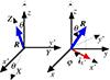 |
Fig. A.2. Reference frame for the divergence evaluation: General case. |
 (A.14)
where the Δ values are taken along each respective axis.
One has now to rotate this result into the l.o.s. reference frame represented in the right part of Fig. A.2. In this reference frame, the  unit vector along Ox′ has the following coordinates
 (A.15)
Accordingly,
 (A.16)
One has by rotational invariance
 (A.17)
so that finally
![Mathematical equation: $$ \begin{aligned} \mathrm{div}\boldsymbol{H}&= \frac{\Delta _{x}H_{x}^{(m)}}{\Delta x}+\frac{\Delta _{y}H_{y}^{(m)}}{\Delta y}+\frac{\Delta _{z}H_{z}^{(m)}}{\Delta z}+\frac{1}{ \cos \theta } \\&\times \left[ \frac{\Delta _{z}H_{x}^{(m)}}{\Delta z}\sin \theta \cos \varphi +\frac{\Delta _{z}H_{y}^{(m)}}{\Delta z}\sin \theta \sin \varphi \right] \ . \nonumber \end{aligned} $$](/articles/aa/full_html/2025/02/aa48632-23/aa48632-23-eq83.gif) (A.18)
(A.18)
The R vector coordinates can also be expressed as
 (A.19)
Accordingly, the above Eq. (A.18) simply results in Eq. (9) of the paper. The second line accounts for the line formation plane inclination with respect to the line of sight
A.1.3. General case
Let’s introduce the l.o.s. basic unit vectors i, k and ℓ (l.o.s. vector), and let’s consider their projections ip and kp along Oz onto the line formation plane perpendicular to the solar radius unit vector R (see Fig. A.3). ip and kp are not unit vectors and have to be evaluated as follows. Let’s denote by A the extremity of the i vector, and by A′ the extremity of the ip vector. A′ is the projection of A along Oz. The AA′ line of Fig. A.3 is defined by the intersection of the two planes of equations x = 1 and y = 0, respectively. A′ is the intersection of the AA′ line with the line formation plane perpendicular to R whose equation is given above in Eq. (A.1). The coordinates of ip are then
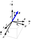 |
Fig. A.3. Projection of the unit vectors of the line of sight reference frame onto the line formation plane, which is perpendicular to the solar radius unit vector, R. |
 (A.20)
Analogously for the k and kp vectors, the BB′ line of Fig. A.3 is defined by the intersection of the two planes of equations x = 0 and y = 1, respectively, and the coordinates of kp are obtained by intersection with the line formation plane given in Eq. (A.1)
 (A.21)
We go on to apply the Ostrogradski’s theorem. The elementary volume is obtained by projecting the elementary surface ΔxΔy along Oz onto the map plane, and by giving it a Δz thickness along Oz. As visible in Fig. A.3, the surface of the projected ΔxΔy is ip Δx × kp Δy, which has for value ΔxΔy/Rz = ΔxΔy/cos θ, where θ is the heliocentric angle. The surfaces of the other sides of the elementary volume are respectively ΔxΔz and ΔyΔz (they are obtained by taking the product of ip or kp with ℓ, which is the unit vector along the l.o.s.). The divergence is then obtained as
![Mathematical equation: $$ \begin{aligned} \mathrm{div}\boldsymbol{H}\ \Delta x\Delta y\Delta z&= \left[ \boldsymbol{H}^{(m)}(z+\Delta z)-\boldsymbol{H}^{(m)}(z)\right] \nonumber \\&\cdot \left[ \boldsymbol{i}_{p}\ \Delta x\times \boldsymbol{k}_{p}\ \Delta y\right] \nonumber \\&+\left[ \boldsymbol{H}^{(m)}(x+\Delta x)-\boldsymbol{H}^{(m)}(x)\right] \nonumber \\&\cdot \left[ \boldsymbol{k}_{p}\ \Delta y\times \boldsymbol{\ell }\ \Delta z\right] \nonumber \\&+\left[ \boldsymbol{H}^{(m)}(y+\Delta y)-\boldsymbol{H}^{(m)}(y)\right] \nonumber \\&\cdot \left[ \boldsymbol{\ell }\ \Delta z\times \boldsymbol{i}_{p}\ \Delta x\right], \end{aligned} $$](/articles/aa/full_html/2025/02/aa48632-23/aa48632-23-eq107.gif) (A.22)
(A.22)
leading to the expression given in Eq. (9). For clarity, the repeated and unchanged indices have been omitted in H(m).
A.2. Calculation of the curl
The curl is similarly obtained by applying Stokes’ theorem, which is that the flux of the curl through an elementary surface equals the “circulation” or work of the vector under study along the frontier of the surface, which is oriented as the surface itself. The elementary surfaces are the different faces of the elementary volume introduced above for the divergence. Analogously to the divergence derivation, we present first below a detailed calculation in the particular case of solar equator (Sect. A.2.1) and then the general case (Sect. A.2.2).
A.2.1. Case of a region located at solar equator
We consider the calculation of JZ from the circulation of H along the oriented frontier of the elementary surface perpendicular to OZ. We have represented this elementary surface in Fig. A.4, which is another view of Fig. A.1. The circulation of H about the oriented surface is given by the scalar products
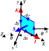 |
Fig. A.4. Elementary surface for the calculation of JZ by applying the Stokes theorem to the circulation of the magnetic field vector along the oriented frontier of the surface. This figure is another view of Fig. A.1. Accordingly, the heliocentric θ angle is oriented by the Oy axis and is negative in the figure. The unit S vector is indeed the same as the unit R vector along the local solar radius. |
![Mathematical equation: $$ \begin{aligned}&\left[ \boldsymbol{H}^{(m)}(y)-\boldsymbol{H}^{(m)}(y+\Delta y)\right] \cdot \boldsymbol{I} \Delta \ell \\&+\left[ \boldsymbol{H}^{(m)}(x+\Delta x)-\boldsymbol{H}^{(m)}(x)\right] \cdot \boldsymbol{K} \Delta y\ . \nonumber \end{aligned} $$](/articles/aa/full_html/2025/02/aa48632-23/aa48632-23-eq111.gif) (A.23)
(A.23)
For clarity, the repeated and unchanged indices have been omitted in H(m). The unit vector I along OX has the following coordinates in the l.o.s. reference frame Oxyz
 (A.24)
whereas K is
 (A.25)
As a consequence, the circulation of H is
![Mathematical equation: $$ \begin{aligned}&\left[ H_{x}^{(m)}(y)\cos \theta -H_{z}^{(m)}(y)\sin \theta \right] \Delta \ell \nonumber \\&+\left[ H_{y}^{(m)}(x+\Delta x)\right] \Delta y \\&-\left[ H_{x}^{(m)}(y+\Delta y)\cos \theta -H_{z}^{(m)}(y+\Delta y)\sin \theta \right] \Delta \ell \nonumber \\&-\left[ H_{y}^{(m)}(x)\right] \Delta y\ . \nonumber \end{aligned} $$](/articles/aa/full_html/2025/02/aa48632-23/aa48632-23-eq118.gif) (A.26)
(A.26)
This circulation equals the flux of J through the surface, which is JZ times the surface value, which is ΔℓΔy = ΔxΔy/cos θ following Eq. (A.9). This can be written as
![Mathematical equation: $$ \begin{aligned} J_{Z}&= \cos \theta \left[ \frac{\Delta _{x}H_{y}^{(m)}}{\Delta x}- \frac{\Delta _{y}H_{x}^{(m)}}{\Delta y}\right] \nonumber \\&+\sin \theta \frac{\Delta _{y}H_{x}^{(m)}}{\Delta y}\ , \end{aligned} $$](/articles/aa/full_html/2025/02/aa48632-23/aa48632-23-eq120.gif) (A.27)
(A.27)
which is Eq. (14) of the paper in the case of the surface located at equator, where the coordinates of the R vector are given by Eq. (A.19) with φ = 0.
A.2.2. General case
Referring now to Fig. A.3, the sides of the elementary volume are respectively ipΔx, kpΔy and ℓ Δz. The circulation of H is given by its scalar product with each of these elementary vectors, eventually reversed following the surface orientation. This leads to
![Mathematical equation: $$ \begin{aligned} J_{Z}\ \frac{\Delta x\Delta y}{R_{z}}&= \boldsymbol{J}\cdot \left[ \boldsymbol{i}_{p}\ \Delta x\times \boldsymbol{k}_{p}\ \Delta y\right] \\&= \left[ \boldsymbol{H}^{(m)}(y)-\boldsymbol{H}^{(m)}(y+\Delta y)\right] \cdot \boldsymbol{i} _{p}\ \Delta x \nonumber \\&+\left[ \boldsymbol{H}^{(m)}(x+\Delta x)-\boldsymbol{H}^{(m)}(x)\right] \cdot \boldsymbol{k} _{p}\ \Delta y \nonumber \end{aligned} $$](/articles/aa/full_html/2025/02/aa48632-23/aa48632-23-eq126.gif) (A.28)
(A.28)
which results in the expression given in Eq. (14). The flux through the two other faces, which are respectively perpendicular to the Ox and Oy of the line of sight reference frame, gives the current components along those axes
![Mathematical equation: $$ \begin{aligned} J_{y}\ \Delta x\Delta z\&= \boldsymbol{J}\cdot \left[ \boldsymbol{\ell }\ dz\times \boldsymbol{i}_{p}\ \Delta x\right] \\&= \left[ \boldsymbol{H}^{(m)}(z+\Delta z)-\boldsymbol{H}^{(m)}(z)\right] \cdot \boldsymbol{i} _{p}\ \Delta x \nonumber \\&+\left[ \boldsymbol{H}^{(m)}(x)-\boldsymbol{H}^{(m)}(x+\Delta x)\right] \cdot \boldsymbol{\ell } \ \Delta z \nonumber \end{aligned} $$](/articles/aa/full_html/2025/02/aa48632-23/aa48632-23-eq127.gif) (A.29)
(A.29)
and
![Mathematical equation: $$ \begin{aligned} J_{x}\ \Delta y\Delta z\&= \boldsymbol{J}\cdot \left[ \boldsymbol{k}_{p}\ \Delta y\times \boldsymbol{\ell }\ \Delta z\right] \\&= \left[ \boldsymbol{H}^{(m)}(z)-\boldsymbol{H}^{(m)}(z+\Delta z)\right] \cdot \boldsymbol{k} _{p}\ \Delta y \nonumber \\&+\left[ \boldsymbol{H}^{(m)}(y+\Delta y)-\boldsymbol{H}^{(m)}(y)\right] \cdot \boldsymbol{\ell } \ \Delta z\ . \nonumber \end{aligned} $$](/articles/aa/full_html/2025/02/aa48632-23/aa48632-23-eq128.gif) (A.30)
(A.30)
This results in the expressions given in Eqs. (15-16). Again, for clarity, the repeated and unchanged indices have been omitted in H(m). These three derived current density vector coordinates are not all taken in the same reference frame. The frame rotation is fully accounted for in Sect. 4.3, where all the coordinates of the current density vector are finally derived in both reference frames.
All Tables
Performance metrics for the limited resolution case for our DIVB resolution algorithm applied to the test data of Leka et al. (2009) and Crouch (2013).
Performance metrics for the noise-added case for our DIVB resolution algorithm applied to the test data provided by K.D. Leka’s courtesy.
All Figures
|
Fig. 1.
|
| In the text | |
|
Fig. 2. Contribution functions of the two lines Fe I 6302.5 Å and 6301.5 Å as a function of the height above τ5000 = 1. The heights where τ = 1, which is the line formation height in the Eddington-Barbier approximation, are indicated by arrows. |
| In the text | |
|
Fig. 3. Result of the ambiguity resolution test using our method applied to theoretical data. Top: Map of the input magnetic field vector. Middle: ambiguity resolution by applying the usual divergence formula (first line of Eq. (9) only) to these data, where the region is assumed to be out of disk center and where two lines formed at two different altitudes are supposed to be observed. Bottom: Ambiguity resolution by applying Eq. (9). |
| In the text | |
|
Fig. 4. Active region NOAA 11420 observed by HINODE/SOT/SP on February 18, 2012 between 11:08 and 12:04 UT. The ambiguity is resolved by our method. Left: Magnetic field vector, vertical component between −2040 and +2040, horizontal component maximum arrow length 1355 G. Middle: current density vector, vertical component between −64 and +64, horizontal component typical arrow length 5000 mA/m2. Right: Lorentz force vector, vertical component between −448 and +448, horizontal component typical arrow length 800 mN/m2. The spatial resolution was reduced by a factor 5 × 5 for paper file size purposes (color figure on-line). |
| In the text | |
|
Fig. 5. Active region NOAA 11494 observed by HINODE/SOT/SP on June 7, 2012 between 14:15 and 15:05 UT. The ambiguity is resolved by our method. Left: magnetic field vector, vertical component between −2150 and +2150, horizontal component maximum arrow length 1743 G. Middle: Current density vector, vertical component between −219 and +219, horizontal component typical arrow length 5000 mA/m2. Right: Lorentz force vector, vertical component between −682 and +682, horizontal component typical arrow length 800 mN/m2. The spatial resolution was reduced by a factor 5 × 5 for paper file size purposes (color figure on-line). |
| In the text | |
|
Fig. 6. Active region NOAA 11476 observed by HINODE/SOT/SP on May 12, 2012 between 02:38 and 03:11 UT. The ambiguity is resolved by our method. Left: Magnetic field vector, vertical component between −2450 and +2450, horizontal component maximum arrow length 2470 G. Middle: current density vector, vertical component between −218 and +218, and horizontal component typical arrow length 8000 mA/m2. Right: Lorentz force vector, vertical component between −1040 and +1040, and horizontal component typical arrow length 800 mN/m2. The spatial resolution was reduced by a factor 5 × 5 for paper file size purposes (color figure online). |
| In the text | |
|
Fig. 7. Active region NOAA 11429 observed by HINODE/SOT/SP on March 6, 2012 between 22:10 and 22:43 UT. The ambiguity is resolved by our method. Left: Magnetic field vector, vertical component between −2480 and +2480, horizontal component maximum arrow length 2441 G. Middle: Current density vector, vertical component between −185 and +185, horizontal component typical arrow length 5000 mA/m2. Right: Lorentz force vector, vertical component between −1180 and +1180, and horizontal component typical arrow length 800 mN/m2. The spatial resolution was reduced by a factor 5 × 5 for paper file size purposes (color figure online). |
| In the text | |
|
Fig. 8. Active region NOAA 11857 observed with THEMIS on October 7, 2013 between 08:57 and 09:22 UT, in the photospheric lines Fe I 6301/6302. The ambiguity is resolved by our method. Left: Magnetic field vector, vertical component between −1790 and +1790, and horizontal component maximum arrow length 1070 G. Middle: Current density vector, vertical component between −68 and +68, and horizontal component maximum arrow length 746 mA/m2. Right: Lorentz force vector, vertical component between −56 and +56, and horizontal component maximum arrow length 133 mN/m2 (color figure online). |
| In the text | |
|
Fig. 9. Active region NOAA 11865 observed with THEMIS on October 11, 2013 between 09:39 and 09:59 UT, in the photospheric lines Fe I 6301/6302. The ambiguity is resolved by our method. Left: Magnetic field vector, vertical component between −1450 and +1450, and horizontal component maximum arrow length 1320 G. Middle: Current density vector, vertical component between −96 and +96, and horizontal component maximum arrow length 655 mA/m2. Right: Lorentz force vector, vertical component between −83 and +83, and horizontal component maximum arrow length 43 mN/m2 (color figure on-line). |
| In the text | |
|
Fig. A.1. Reference frame for the divergence evaluation: case of an observation at the solar equator. The heliocentric θ angle is oriented by the Oy axis and is negative in the figure. The two formation planes corresponding to the two lines (1) and (2) are indicated by their respective number. The unit S vector is indeed the same as the unit R vector along the local solar radius. |
| In the text | |
|
Fig. A.2. Reference frame for the divergence evaluation: General case. |
| In the text | |
|
Fig. A.3. Projection of the unit vectors of the line of sight reference frame onto the line formation plane, which is perpendicular to the solar radius unit vector, R. |
| In the text | |
|
Fig. A.4. Elementary surface for the calculation of JZ by applying the Stokes theorem to the circulation of the magnetic field vector along the oriented frontier of the surface. This figure is another view of Fig. A.1. Accordingly, the heliocentric θ angle is oriented by the Oy axis and is negative in the figure. The unit S vector is indeed the same as the unit R vector along the local solar radius. |
| In the text | |
Current usage metrics show cumulative count of Article Views (full-text article views including HTML views, PDF and ePub downloads, according to the available data) and Abstracts Views on Vision4Press platform.
Data correspond to usage on the plateform after 2015. The current usage metrics is available 48-96 hours after online publication and is updated daily on week days.
Initial download of the metrics may take a while.