| Issue |
A&A
Volume 693, January 2025
|
|
|---|---|---|
| Article Number | A183 | |
| Number of page(s) | 6 | |
| Section | Celestial mechanics and astrometry | |
| DOI | https://doi.org/10.1051/0004-6361/202451385 | |
| Published online | 15 January 2025 | |
Asteroid detection polar equation calculation and graphical representation
1
Planetary Defence Office, ESA/ESOC,
Robert-Bosch-Straße 5,
64293
Darmstadt,
Germany
2
NEO Coordination Centre, Planetary Defence Office, ESA/ESRIN,
Largo Galileo Galilei, 1,
00044
Frascati,
Italy
3
Planetary Defence Office, ESA/ESAC, Camino bajo del Castillo, s/n,
28692
Villanueva de la Cañada,
Spain
4
Division for Medical Radiation Physics and Space Environment, Carl von Ossietzky Universität Oldenburg,
26111
Oldenburg,
Germany
★ Corresponding author; This email address is being protected from spambots. You need JavaScript enabled to view it.
Received:
4
July
2024
Accepted:
3
December
2024
Abstract
Context. The observability of an asteroid from the ground depends on the distance to the Sun and the observer, on the phase angle, on the object shape, and on its surface reflectivity properties. Several magnitude systems have been proposed in the past decades to model the visual magnitude of the object based on these parameters.
Aims. Independently of the magnitude system, there is a three-dimensional representation of the geometrical locus of equal visual magnitude when this value is constrained for a given asteroid. We called this the detection polar curve, or just, the detection polar. We derived a process in order to represent it graphically.
Methods. We analysed the shape of this geometrical locus for the H, G magnitude system and determined its applicability to the representation of the detectability of an asteroid in its trajectory. We thus calculated the asteroid detection polar equation, as well as the threshold values that change the type of asteroid detectability solution.
Results. The resulting detection polar is discussed, the synodic orbit visualisation tool is introduced, as are examples of how it can be used to analyse the graphical representation of an asteroid trajectory, and to represent the detection polar for a given limiting visual magnitude.
Key words: virtual observatory tools / celestial mechanics / minor planets, asteroids: general
© The Authors 2025
 Open Access article, published by EDP Sciences, under the terms of the Creative Commons Attribution License (https://creativecommons.org/licenses/by/4.0), which permits unrestricted use, distribution, and reproduction in any medium, provided the original work is properly cited.
This article is published in open access under the Subscribe to Open model. This email address is being protected from spambots. You need JavaScript enabled to view it. to support open access publication.
1 Introduction
The visual observability of an asteroid depends on the distance of the object to the Sun and to the observation point, on the asteroid phase angle, its shape and rotation state, and on the surface physical properties of the object. Several models were proposed in order to represent the visual magnitude as a function of these variables, examples of which are the H, G magnitude system proposed by Bowell et al. (1989), the H, G1, G2 and the H, G12 systems by Muinonen et al. (2010), and the ![Mathematical equation: $\[H, G_{12}^{*}\]$](/articles/aa/full_html/2025/01/aa51385-24/aa51385-24-eq1.png) system by Penttilä et al. (2016). The recent sHG1G2 model has been proposed to account for brightness changes caused by the spin orientation and polar oblateness (Carry et al. 2024). We analysed the observational geometrical 3D shape associated with the widely used H, G model in detail and assumed a limiting visual magnitude of the observational equipment as the constraint. These shapes were previously analysed by Cano & Bastante (2014) and Denneau (2015), but we provide a systematic and complete method for the calculation and representation of these shapes here.
system by Penttilä et al. (2016). The recent sHG1G2 model has been proposed to account for brightness changes caused by the spin orientation and polar oblateness (Carry et al. 2024). We analysed the observational geometrical 3D shape associated with the widely used H, G model in detail and assumed a limiting visual magnitude of the observational equipment as the constraint. These shapes were previously analysed by Cano & Bastante (2014) and Denneau (2015), but we provide a systematic and complete method for the calculation and representation of these shapes here.
The Planetary Defence Office (PDO) at the European Space Agency (ESA) has implemented the synodic orbit visualisation tool (SOVT) for the above purpose. This software tool allows the graphical representation of the described 3D shapes in addition to the representation of the motion of near-Earth objects (NEO) in space in a so-called co-rotational reference frame, which is a frame centred at the Sun and rotating following the translational motion of the Earth. The SOVT allows anyone to analyse in a very direct and intuitive way when and how an asteroid or a comet becomes observable from Earth by a given telescope.
2 Methods
2.1 Ecliptic projection of an NEO observability region
Without loss of generality, we assumed that an observer moves around the Sun on an Earth-like circular orbit with a radius of 1 au. We considered a Sun-centred reference system whose x-axis is oriented in the direction of the moving observer, the y-axis lies within the ecliptic plane, and the z-axis in the direction of the ecliptic north pole. In this rotating reference system, we can pursue the representation of the geometrical locus of points with an equal visual magnitude under a given asteroid photometric model.
We focused on achieving the representation of this geometrical locus as based on the H, G magnitude system and for given values of the limiting visual magnitude of the observer. In this context, we assumed an asteroid with an absolute magnitude H and a slope parameter G. When the object is located at a distance d from the Sun and at a distance Δ from the Earth, and has a phase angle α, the resulting visual magnitude can be computed as given in Bowell et al. (1989),
![Mathematical equation: $\[V(\alpha)=H-2.5 ~\log _{10} F(\alpha)+5 ~\log _{10}~(d \Delta),\]$](/articles/aa/full_html/2025/01/aa51385-24/aa51385-24-eq2.png) (1)
(1)
where
![Mathematical equation: $\[F(\alpha)=(1-G) \phi_{1}(\alpha)+G \phi_{2}(\alpha),\]$](/articles/aa/full_html/2025/01/aa51385-24/aa51385-24-eq3.png) (2)
(2)
and where the functions ϕi with i = 1, 2 are defined by
![Mathematical equation: $\[\phi_{i}(\alpha)=W(\alpha) \phi_{i S}(\alpha)+(1-W(\alpha)) \phi_{i L}(\alpha),\]$](/articles/aa/full_html/2025/01/aa51385-24/aa51385-24-eq4.png) (3)
(3)
![Mathematical equation: $\[W(\alpha)=\exp \left(-90.56 ~\tan ^{2} \frac{\alpha}{2}\right)\]$](/articles/aa/full_html/2025/01/aa51385-24/aa51385-24-eq5.png) (4)
(4)
![Mathematical equation: $\[\phi_{i S}(\alpha)=1-\frac{C_{i} ~\sin~ \alpha}{0.119+1.341 ~\sin~ \alpha-0.754 ~\sin ^{2} \alpha}\]$](/articles/aa/full_html/2025/01/aa51385-24/aa51385-24-eq6.png) (5)
(5)
![Mathematical equation: $\[\phi_{i L}(\alpha)=\exp \left(-A_{i}\left(\tan \frac{\alpha}{2}\right)^{B_{i}}\right)\]$](/articles/aa/full_html/2025/01/aa51385-24/aa51385-24-eq7.png) (6)
(6)
with the parameters A1 = 3.332, A2 = 1.862, B1 = 0.631, B2 = 1.218, C1 = 0.986, and C2 = 0.238.
When we fixed the value of Vlim as the one achievable by a given telescope, a solution for the distance product dΔ can be found as a function of α by computing the solution of this equation,
![Mathematical equation: $\[d \Delta=10^{\left(V_{l i m}-H+2.5 ~\log _{10} F(\alpha)\right) / 5}.\]$](/articles/aa/full_html/2025/01/aa51385-24/aa51385-24-eq8.png) (7)
(7)
The solution can be parametrised through a representation in polar coordinates from the mid-point between the observer and the Sun. However, another more graphical way to consider the solutions to the above equation is to observe that the geometrical locus of solutions can be derived by searching for the intersection of the curve of constant phase angle with the curve of constant value of the distance product derived from the previous equation. When we consider the first curve and a 2D representation, the geometrical locus of points that see the segment between the Sun and the observer with the same phase angle α is trivial and is formed by two arcs of a circle that pass by both the Sun and the observer, one on the positive side of the y-axis and a symmetric one on the negative side, as shown in Fig. 1 for different values of α and assuming the point in the middle of the segment joining both focal points as the origin.
Starting with a very small phase angle, the radius of the two circular arcs will be large. As the phase angle increases, the radius of the arcs will diminish. When the phase angle reaches 90°, the two arcs will form a perfect circumference passing by the Sun and the observer. As the phase angle continues to increase, the circular arcs will be smaller than half a circumference and will continue to increase in diameter. At the limit of 180°, the solution will have degenerated into a line segment that connects the observer and the Sun. It is noted that the geometrical solution to the iso-angle locus is symmetric with respect to the abscissa axis and with respect to a vertical line passing at half the distance between the Sun and the observer.
Regarding the geometrical locus of the points that have an equal product of the distances to the Sun and the observer, this is represented by the so-called Cassini ovals, as shown in Fig. 2 for different values of ρ, which is the square root of the distance product and the sizing parameter for the ovals.
The Cassini ovals have two types of solutions depending on the value of ![Mathematical equation: $\[e=\frac{\rho}{\delta}\]$](/articles/aa/full_html/2025/01/aa51385-24/aa51385-24-eq9.png) , where δ is the semi-distance between the two focal points, which in this case is δ = 0.5. When e < 1, the solutions are two disconnected ovals close to each of the two focal points, when e = 1, the solution is the lemniscate of Bernoulli, and when e > 1, the curve is a single connected loop enclosing the two focal points.
, where δ is the semi-distance between the two focal points, which in this case is δ = 0.5. When e < 1, the solutions are two disconnected ovals close to each of the two focal points, when e = 1, the solution is the lemniscate of Bernoulli, and when e > 1, the curve is a single connected loop enclosing the two focal points.
As in the previous case, the geometrical solution to the iso-product locus is symmetric with respect to the abscissa axis and with respect to a vertical line passing at half the distance between the Sun and the observer. Therefore, the solution that corresponds to the intersection of the iso-angle curves with the iso-product curves will also have the same symmetry properties. This also means that in general, the intersection of the two sets of curves will be a set of four points for each value of the phase angle.
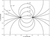 |
Fig. 1 Schematic representation of the geometrical locus of an equal phase angle for different values of α. The origin of the reference system is located at the mid-point between the focal points. |
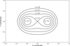 |
Fig. 2 Schematic representation of the geometrical locus of an equal product of the distance to the Sun and the distance to the observer for different values of ρ. The origin of the reference system is located at the mid-point between the focal points. |
2.2 The detection polar
When we consider all the above geometrical elements and given an asteroid with the mentioned values of H and G and an observational asset with a limiting visual magnitude Vlim, Eq. (7) allows us to obtain the resulting geometrical locus by varying the phase angle between 0° and 180°. We called this geometrical locus the detection polar. In the area within the detection polar, the object can be observed by the selected telescope. Outside of the area, the visual magnitude is fainter than the limiting value, and the object is therefore not observable. As previously commented, the solution is symmetrical with respect to the x-axis and with respect to a perpendicular line passing by the mid distance between the observer and the Sun. The solution is dependent on only two parameters: B = (Vlim − H), and G. In the following, we assume a value of G = 0.15 and vary the value of B. Further to the above, it is known that in the H − G model 120° in phase angle should not be exceeded, but we decided to extend the calculation of the detection polar up to 180° for completeness, but in the knowledge of this limitation.
Fig. 3 provides a series of plots with the 2D evolution of the detection polar for different values of the relative magnitude B starting from −2.0 and up to +4.0 in steps of one magnitude. Different to the previous plots, the Sun is now located at the origin, and the Earth lies at point (1, 0). An additional case is provided for a threshold value of Bthr = 1.66875, which corresponds to the transition from two independent separated regions to one overarching region. Starting with B = −2.0, two heart-like solutions are located at each of the focal points, and the tip of the heart points in the direction of the opposition effect, corresponding to a zero phase angle. As the value of the relative magnitude grows, the size of the two shapes increases accordingly. When B reaches the mentioned value of 1.66875, the two shapes make contact, and they transform into two other shapes; an external shape that continues to grow, and an internal shape that joins the two focal points and decreases in size as the relative magnitude grows. An example of the visible region is provided in grey in Fig. 4 for a value of B = 3.0.
At this point, no visibility constraints other than the mentioned magnitude system were applied in Figs. 3 and 4. However, it is expected that the derived solution close to the Sun is affected by a low solar elongation as seen from the Earth, thus limiting the possibilities of observing this part of the detection polar. This can easily be represented in these figures by defining the given limiting solar elongation and drawing the corresponding straight lines from the Earth in the semi-space at the side of the Sun, as observable in Fig. 5 for a 45° elongation cone. This shape would turn into a 3D cone when this representation were extended to three dimensions. Independently of this, it is also expected that some parts of the detection polar section close to the Sun become visible as the limiting visual magnitude of the telescope is increased. This is particularly obvious when the two shapes join to form the evolved detection polar shape above Bthr = 1.66875.
The mentioned transition value Bthr applies to a value of G = 0.15. For a more general derivation of Bthr, we need to find the solutions that allow the detection polar curves to reach the line equidistant to the focal points, which is a line passing by the point ![Mathematical equation: $\[(\frac{1}{2}, 0)\]$](/articles/aa/full_html/2025/01/aa51385-24/aa51385-24-eq10.png) . In this case, dΔ = ρ2, and together with Eq. (7), this leads to
. In this case, dΔ = ρ2, and together with Eq. (7), this leads to
![Mathematical equation: $\[\rho^{2}=10^{\left(B+2.5 \log _{10} F(\alpha)\right) / 5}.\]$](/articles/aa/full_html/2025/01/aa51385-24/aa51385-24-eq11.png) (8)
(8)
Eq. (8) can also be expressed as
![Mathematical equation: $\[\rho=F(\alpha)^{1 / 4} 10^{B / 10}.\]$](/articles/aa/full_html/2025/01/aa51385-24/aa51385-24-eq12.png) (9)
(9)
Then, taking the distance equation from a point in the equidistant line,
![Mathematical equation: $\[\rho ~\sin~ (\alpha / 2)=1 / 2,\]$](/articles/aa/full_html/2025/01/aa51385-24/aa51385-24-eq13.png) (10)
(10)
we can substitute the value of ρ from Eqs. (9) into (10) to find an expression relating the solution of B as function of the phase angle,
![Mathematical equation: $\[B=-10 ~\log _{10}\left(2 F(\alpha)^{1 / 4} ~\sin (\alpha / 2)\right).\]$](/articles/aa/full_html/2025/01/aa51385-24/aa51385-24-eq14.png) (11)
(11)
This function is defined in the whole range of phase angles and in a range of B ≥ Bthr. For B = Bthr, there is a single solution of α, whereas there are two solutions for B > Bthr. This can be observed in Fig. 6, where the resulting curves of the B parameter as a function of α are represented for values of G equal to 0.0, 0.15, and 0.30. The resulting values of Bthr for these examples are 2.10878, 1.66875, and 1.35619, respectively. This behaviour is compatible with the fact that when the polar sections coalesce and thus B > Bthr, there are two intersections with the central axis in the positive size of the abscissa semi-plane and another two symmetric in the negative semi-plane. From the previous discussion, we infer that the extension to 3D of the detection polar can be easily achievable, as there is cylindrical symmetry of the shape with respect to the x-axis.
 |
Fig. 3 Planar detection polars for values of the relative magnitude B between −2 and +1 (left) and B between +1.66875 and +4 (right), and for G = 0.15. |
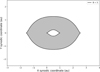 |
Fig. 4 Planar detection polar for a value of the relative magnitude of B = 3 and marking the observable region (in grey). |
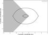 |
Fig. 5 Planar detection polar for a value of the relative magnitude of B = 3 and a 45° solar elongation exclusion cone (in grey). |
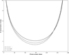 |
Fig. 6 Curves of the B parameter as a function of the phase angle for values of G of 0.0, 0.15, and 0.3. |
3 ESA synodic orbit visualisation tool
In an effort to allow independent users to generate the graphical representation of the co-rotating trajectory of an NEO in the mentioned synodic reference system and the representation of the proposed detection polar, ESA has developed the synodic orbit visualisation tool1. The SOVT is one of several utilities developed at the ESA NEO Coordination Centre and is included in the so-called NEO Toolkit2.
The NEO Toolkit is a public set of web-based tools designed to facilitate the computation of observational constraints and the graphical representation of several types of data, all focused on NEOs. Currently, the NEO Toolkit is composed of five independent tools:
The orbit visualisation tool (OVT),
the flyby visualisation tool (FVT),
the observation planning tool (OPT),
the sky chart visualisation tool (SCDT), and
the synodic orbit visualisation tool (SOVT).
Briefly, the OVT delivers a 3D graphical representation of the Solar System, displaying the Keplerian and perturbed orbits of NEOs, among other asteroid groups and families. The FVT zooms in the vicinity of the Earth to show the orbits or fly-bys of the NEOs that closely approach Earth within three lunar distances. The OPT provides high-precision ephemeris calculations for any NEO at any date and location of the globe. The SCDT works similarly to the OPT, but locates the objects in a virtual sky dome.
The SOVT, among other features, allows the users to display the synodic trajectory of an object and to represent the detection polar in the Sun-Earth reference system. As discussed in the previous section, in the H − G magnitude system, the detection polar can be computed after the user manually defines the limiting visual magnitude Vlim, that is the observational capability of a telescope on Earth. A snapshot of the detection polar for a case with B < Bthr, that is, with one part bound to Earth and the other bound to the Sun, is provided in Fig. 7. The selected object for this example is 1993 FA1, which has H = 25.991, an orbital period of 1.703 years, and a synodic period of 2.422 years, propagated for ten years. The limiting magnitude of the telescope was taken as Vlim = 26.0, and we thus achieve an almost null value of B. The solution bound to Earth intersects a portion of the object trajectory (in light blue), implying that the object might be observable in this particular period of time with a telescope of this capability. The tool also allows us to represent a cone with a limiting elongation from the Sun and the timely evolution of several ancillary variables, such as the distance to Earth, the phase angle, and the visual magnitude.
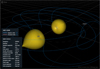 |
Fig. 7 Snapshot of the SOVT providing a ten-year Keplerian trajectory for 1993 FA1. The detection polar shapes are defined with Vlim = 26.0. |
4 Examples
4.1 Discovery of (99942) Apophis
Asteroid (99942) Apophis, probably the most famous NEO of the past decades, was first discovered as a low-elongation object from Kitt Peak (Arizona, USA) on 19 June 2004. Follow-up on the following night was sufficient to provide an indication of an NEO orbit, but the object was subsequently lost due to poor weather. A synodic plot shows that the early 2004 observing opportunity, while still challenging due to the low solar elongation and moderate faintness (V ~ 21), was indeed the first opportunity to easily observe the object since the late 1990s, when major NEO surveys began to operate. This is due to a synodic period of about eight years, which is a consequence of the orbital period of the object of about T = 324 days.
After it was lost in June 2004, Apophis was serendipitously rediscovered on 18 December 2004 from Siding Spring (Australia), as shown in Fig. 8. When combined with the June detections, the two datasets resulted in a significant impact chance with Earth in 2029, roughly three synodic periods (24 years) after discovery. The late 2004 apparition corresponded to a close approach of the object to our planet, and unusually easy observability circumstances, as again clearly shown in the synodic plot. This ensured an easy observability of the object in late 2004, and together with prediscovery observations from March 2004, this led to the exclusion of the possible impact in 2029 (Sansaturio & Arratia 2008).
However, impact solutions for later years remained even after the easy observability in 2005 and 2006. By early 2007, the object started to recede from Earth and head towards solar conjunction. The subsequent observability window occurred, as expected, roughly eight years later (one synodic period), in 2012–2013 (Farnocchia et al. 2013; Tholen et al. 2013). Despite excellent observational coverage, it was not yet possible to exclude all possible impact solutions over the next century by the time the observing window closed again. The final signal that all threat had passed for Apophis had to wait one more synodic cycle and only came in 2020 as the result of additional high-precision observations (Reddy et al. 2022).
The case of Apophis clearly exemplifies the importance of an early discovery for a possibly dangerous asteroid: In many cases, no observational opportunities are present, and critical objects may remain unobservable for many years between short observability windows. When this happens, valuable observations can only rarely be obtained, and it may be necessary to wait many decades (or many synodic periods) before the threat is clarified.
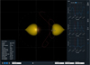 |
Fig. 8 Snapshot of the SOVT representing asteroid (99942) Apophis between 1 January 2004 and 31 December 2006 and with a telescope with Vlim = 19.0, which is close to the value at recovery in December 2004. It was recovered around the minimum visual magnitude in the period. |
4.2 The case of (367943) Duende
Asteroid (367943) Duende was discovered from Observatorio Astronómico de Mallorca (OAM) at La Sagra (Spain) on 23 February 2012 and was quickly determined to have a very close approach to Earth one year later, on 15 February 2013, which by chance was the same day as the Chelyabinsk asteroid impacted on Earth. The close-approach distance was 34048 km, which is smaller than the distance to the geostationary ring. This NEO has an absolute magnitude H = 24.05, and before the close approach to Earth in 2013, it was an Apollo asteroid with a perihelion distance q = 0.893 au, an aphelion distance Q = 1.110 au, a minimum orbit intersection distance (MOID) of 0.00035 au, and an orbital period of T = 366.25 days, which implied a very long synodic period that exceeded one century. The object was almost an Earth co-orbital, as shown in Fig. 9. During the discovery apparition, measurements were collected until 12 May 2012, when it had faded to magnitude 24. The detection polar represented in Fig. 9 corresponds to a limiting magnitude of 19, which is close to the magnitude at discovery.
The second observability period was opened with the recovery of the object on 9 January 2013 with the 6.5 m Magellan-Baade telescope at Las Campanas Observatory (Chile), again around visual magnitude 24, as the object entered the detection polar from the southern hemisphere at this limiting value. The observations ended after its closest approach to Earth, and the latest observations were collected on 21 February 2013. Because the distance at close approach was so small, this apparition included both optical and radar measurements. The close approach to Earth transformed the object into an Aten with q = 0.829 au and Q = 0.991 au, an MOID of 0.00040 au, and an orbital period of T = 317.16 days, resulting in a new synodic period of just 6.60 yr. Thus, the object lost its almost co-orbital motion with Earth in favour of a slightly eccentric orbit, with the aphelion close to 1 au. The next close approach to Earth will be on 15 February 2046 at 0.0149 au.
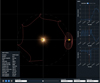 |
Fig. 9 Snapshot of the SOVT representing asteroid (367943) Duende between 1 January 2007 and 1 January 2018 and with a telescope with Vlim = 19.0. The trajectory transforms from a long synodic period Apollo orbit into a relatively short synodic period Aten orbit. |
4.3 The case of (614689) 2020 XL5, an Earth Trojan
Asteroid (614689) 2020 XL5 was discovered by the Pan-STARRS 1 telescope on 12 December 2020 and was determined to be an Earth Trojan a few months later (Santana-Ros et al. 2022; Hui et al. 2021). When its motion is displayed in a synodic plot as in Fig. 10, the Trojan nature of the object is immediately clear. It results in a bean-shaped nearly closed trajectory roughly centred around the L4 Lagrangian point of Earth. The plot is non-trivial, however, because it clearly shows that even Earth Trojan asteroids do not maintain a constant observability geometry when seen from Earth: Their libration around the L4 point is significant, resulting in a large variability in the geocentric distance and in the solar elongation of the object. An elongation cone with an angle of 60° from the Sun is represented in the figure by means of a shaded region. Because of these constraints, Trojan asteroids are often challenging to follow up, with short observational opportunities that last a few days or weeks every year. In the case of 2020 XL5, this visibility period typically occurs every year between November and February of the next year.
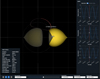 |
Fig. 10 Snapshot of the SOVT representing asteroid (614689) 2020 XL5 between 1 July 2019 and 1 July 2022 and with a telescope with Vlim = 21.6, close to the value at discovery. A solar elongation cone of 60° is represented in grey. The trajectory is only visible from Earth in a small part of its motion around the L4 Lagrangian point. |
4.4 The case of (469219) Kamo‘oalewa, an Earth co-orbital
Asteroid Kamo‘oalewa was discovered by Pan-STARRS 1 at Haleakala Observatory on 27 April 2016 and was determined to have an orbital period very close to that of Earth. After its discovery, precovery observations taken by the Sloan Digital Sky Survey (SDSS) in 2004 and by the discovery station between 2011 and 2016, among others, were identified. Its period, eccentricity, and inclination show that it is indeed on an Earth quasi-satellite orbit, as shown in Fig. 11. The object appears to be orbiting Earth in the synodic reference frame because the difference in the mean longitude of the asteroid and Earth librates around zero. However, (469219) Kamo‘oalewa is not gravitationally bound to Earth because it is well beyond its sphere of influence. The orbit was found to be stable in the last century and will be stable for the next centuries (de la Fuente Marcos & de la Fuente Marcos 2016; Fenucci & Novaković 2021).
The synodic orbit is located between Sun and Earth in its southern excursions and beyond Earth in its northern branches. This means that the orbit is typically observable by northern observatories recurrently between the months of March and May, whereas the southern part remains at low solar elongation angles. For an observatory with a limiting magnitude of 22, it is possible to clearly observe this observational pattern because the detection polar is typically intersected in the mentioned time interval.
5 Summary
Observability of asteroids from Earth is the result of the combination of the trajectory conditions with respect to our planet and the detection capabilities of the telescopes used on the ground. A proper graphical representation of how these visibility conditions map in space, which we called the detection polar, allows us to understand very straightforwardly which parts of the trajectory of an asteroid will be visible from a given observation point.
The characterisation of the 3D geometrical solution for detectability was the purpose of this work, together with the presentation of the ESA synodic orbit visualisation tool. This tool allows us, and any interested user, to gather the representation of asteroid trajectories in a synodic reference frame and to graphically render the detection polar for a given telescope.
Furthermore, we provided examples of relevant asteroid cases such as (99942) Apophis, (367943) Duende, (614689) 2020 XL5, and (469219) Kamo‘oalewa. It is expected that the SOVT will not only be a useful tool for the NEO observational community, either professional or amateur, but also for the science outreach community.
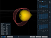 |
Fig. 11 Snapshot of the SOVT representing asteroid (469219) Kamo‘oalewa between 1 January 2010 and 1 January 2031 and with a telescope with Vlim = 22.0. The object is on a quasi-satellite orbit of Earth. |
Acknowledgements
The development of the SOVT has been funded and managed by ESA in an industry contract with Eversis Sp. z o.o. (Poland) and Deimos Space S.R.L. (Romania). The authors are grateful to the quality of the final product developed by both companies.
References
- Bowell, E., Hapke, B., Domingue, D., et al. 1989, in Asteroids II, eds. R. P. Binzel, T. Gehrels, & M. S. Matthews (Tucson: University of Arizona Press), 524 [Google Scholar]
- Cano, J. L., & Bastante, J. C. 2014, in Proceedings of the 24th International Symposium on Space Flight Dynamics [Google Scholar]
- Carry, B., Peloton, J., Montagner, R. L., Mahlke, M., & Berthier, J. 2024, A&A, 687, A38 [NASA ADS] [CrossRef] [EDP Sciences] [Google Scholar]
- de la Fuente Marcos, C., & de la Fuente Marcos, R. 2016, MNRAS, 462, 3441 [CrossRef] [Google Scholar]
- Denneau, L. 2015, IAU Symp., 318, 1 [NASA ADS] [Google Scholar]
- Farnocchia, D., Chesley, S. R., Chodas, P. W., et al. 2013, Icarus, 224, 192 [Google Scholar]
- Fenucci, M., & Novaković, B. 2021, AJ, 162, 227 [NASA ADS] [CrossRef] [Google Scholar]
- Hui, M.-T., Wiegert, P. A., Tholen, D. J., & Föhring, D. 2021, ApJ, 922, L25 [NASA ADS] [CrossRef] [Google Scholar]
- Muinonen, K., Belskaya, I. N., Cellino, A., et al. 2010, Icarus, 209, 542 [Google Scholar]
- Penttilä, A., Shevchenko, V., Wilkman, O., & Muinonen, K. 2016, Planet. Space Sci., 123, 117 [CrossRef] [Google Scholar]
- Reddy, V., Kelley, M. S., Dotson, J., et al. 2022, Planet. Sci. J., 3, 123 [NASA ADS] [CrossRef] [Google Scholar]
- Sansaturio, M. E., & Arratia, O. 2008, Earth Moon Planets, 102, 425 [NASA ADS] [CrossRef] [Google Scholar]
- Santana-Ros, T., Micheli, M., Faggioli, L., et al. 2022, Nat. Commun., 13, 447 [NASA ADS] [CrossRef] [Google Scholar]
- Tholen, D. J., Micheli, M., & Elliott, G. T. 2013, Acta Astron., 90, 56 [NASA ADS] [CrossRef] [Google Scholar]
All Figures
|
Fig. 1 Schematic representation of the geometrical locus of an equal phase angle for different values of α. The origin of the reference system is located at the mid-point between the focal points. |
| In the text | |
|
Fig. 2 Schematic representation of the geometrical locus of an equal product of the distance to the Sun and the distance to the observer for different values of ρ. The origin of the reference system is located at the mid-point between the focal points. |
| In the text | |
|
Fig. 3 Planar detection polars for values of the relative magnitude B between −2 and +1 (left) and B between +1.66875 and +4 (right), and for G = 0.15. |
| In the text | |
|
Fig. 4 Planar detection polar for a value of the relative magnitude of B = 3 and marking the observable region (in grey). |
| In the text | |
|
Fig. 5 Planar detection polar for a value of the relative magnitude of B = 3 and a 45° solar elongation exclusion cone (in grey). |
| In the text | |
|
Fig. 6 Curves of the B parameter as a function of the phase angle for values of G of 0.0, 0.15, and 0.3. |
| In the text | |
|
Fig. 7 Snapshot of the SOVT providing a ten-year Keplerian trajectory for 1993 FA1. The detection polar shapes are defined with Vlim = 26.0. |
| In the text | |
|
Fig. 8 Snapshot of the SOVT representing asteroid (99942) Apophis between 1 January 2004 and 31 December 2006 and with a telescope with Vlim = 19.0, which is close to the value at recovery in December 2004. It was recovered around the minimum visual magnitude in the period. |
| In the text | |
|
Fig. 9 Snapshot of the SOVT representing asteroid (367943) Duende between 1 January 2007 and 1 January 2018 and with a telescope with Vlim = 19.0. The trajectory transforms from a long synodic period Apollo orbit into a relatively short synodic period Aten orbit. |
| In the text | |
|
Fig. 10 Snapshot of the SOVT representing asteroid (614689) 2020 XL5 between 1 July 2019 and 1 July 2022 and with a telescope with Vlim = 21.6, close to the value at discovery. A solar elongation cone of 60° is represented in grey. The trajectory is only visible from Earth in a small part of its motion around the L4 Lagrangian point. |
| In the text | |
|
Fig. 11 Snapshot of the SOVT representing asteroid (469219) Kamo‘oalewa between 1 January 2010 and 1 January 2031 and with a telescope with Vlim = 22.0. The object is on a quasi-satellite orbit of Earth. |
| In the text | |
Current usage metrics show cumulative count of Article Views (full-text article views including HTML views, PDF and ePub downloads, according to the available data) and Abstracts Views on Vision4Press platform.
Data correspond to usage on the plateform after 2015. The current usage metrics is available 48-96 hours after online publication and is updated daily on week days.
Initial download of the metrics may take a while.