| Issue |
A&A
Volume 692, December 2024
|
|
|---|---|---|
| Article Number | A231 | |
| Number of page(s) | 10 | |
| Section | Catalogs and data | |
| DOI | https://doi.org/10.1051/0004-6361/202452075 | |
| Published online | 17 December 2024 | |
A new sample of super-slowly rotating Ap (ssrAp) stars from the Zwicky Transient Facility survey
1
Bundesdeutsche Arbeitsgemeinschaft für Veränderliche Sterne e.V. (BAV),
Munsterdamm 90,
12169
Berlin,
Germany
2
American Association of Variable Star Observers (AAVSO),
49 Bay State Rd,
Cambridge,
MA
02138,
USA
3
Faculty of Science, Masaryk University, Department of Theoretical Physics and Astrophysics,
Kotlářská 2,
611 37
Brno,
Czech Republic
★ Corresponding author; This email address is being protected from spambots. You need JavaScript enabled to view it.
Received:
31
August
2024
Accepted:
31
October
2024
Abstract
Context. The magnetic chemically peculiar Ap stars exhibit an extreme spread of rotational velocities, the cause of which is not clearly understood. Ap stars with rotation periods of 50 days or longer are know as super-slowly rotating Ap (ssrAp) stars. Photometrically variable Ap stars are commonly termed α2 Canum Venaticorum (ACV) variables.
Aims. Our study aims to enlarge the sample of known ssrAp stars using data from the Zwicky Transient Facility (ZTF) survey to enable more robust and significant statistical studies of these objects.
Methods. Using selection criteria based on the known characteristics of ACV variables, candidate stars were gleaned from the ZTF catalogues of periodic and suspected variable stars and from ZTF raw data. ssrAp stars were identified from this list via their characteristic photometric properties, Δa photometry, and spectral classification.
Results. The final sample consists of 70 new ssrAp stars, which mostly exhibit rotation periods of between 50 and 200 days. The object with the longest period has a rotation period of 2551.7 days. We present astrophysical parameters and a Hertzsprung-Russell diagram for the complete sample of known ssrAp stars. With very few exceptions, the ssrAp stars are grouped in the middle of the main sequence with ages in excess of 150 Myr. ZTF J021309.72+582827.7 was identified as a possible binary star harbouring an Ap star and a cool component, possibly shrouded in dust.
Conclusions. With our study, we enlarge the sample of known ssrAp stars by about 150%, paving the way for more in-depth statistical studies.
Key words: stars: chemically peculiar / stars: early-type / stars: rotation / stars: variables: general
© The Authors 2024
 Open Access article, published by EDP Sciences, under the terms of the Creative Commons Attribution License (https://creativecommons.org/licenses/by/4.0), which permits unrestricted use, distribution, and reproduction in any medium, provided the original work is properly cited.
This article is published in open access under the Subscribe to Open model. This email address is being protected from spambots. You need JavaScript enabled to view it. to support open access publication.
1 Introduction
Ap/CP2 stars are chemically peculiar (CP) stars of the upper main sequence (spectral types late-B to early-F) defined by the presence of peculiarly strong (or weak) absorption lines of certain elements such as Si, Fe, Cr, Sr, or Eu in their spectra (e.g. Preston 1974; Renson & Manfroid 2009).
They possess strong, globally organised magnetic fields (~300 G to several tens of kiloGauss; e.g. Babcock 1958; Borra & Landstreet 1980; Mathys 1991; Mathys et al. 1997; Romanyuk et al. 2014, 2015, 2016, 2017, 2018, 2020, 2022a,b, 2023; Bagnulo et al. 2015) and exhibit a non-uniform surface distribution of chemical elements, which leads to strictly periodic changes in the spectra and brightness of many Ap stars that are satisfactorily explained by the oblique rotator model (Stibbs 1950). The observed photometric variability results from a flux redistribution in the unevenly distributed surface abundance patches (‘chemical spots’) of certain elements (e.g. Wolff & Wolff 1971; Molnar 1973; Krtička et al. 2012). This leads to certain peculiarities, such as antiphase variations between different wavelength regions (e.g. Molnar 1973, 1975; Mikulášek et al. 2007; Gröbel et al. 2017) that can be utilised to identify this group of CP stars in the absence of spectroscopic data (Faltová et al. 2021; Bauer-Fasching et al. 2024).
Photometrically variable Ap stars are commonly termed α2 Canum Venaticorum (ACV) variables (Morgan 1933; Kukarkin et al. 1958; International Astronomical Union 1966; Samus et al. 2017). The number of ACV variables with an accurate rotation period determination has increased significantly in recent years through the exploitation of various time-domain photometric surveys. This includes both ground-based surveys (e.g. Bernhard et al. 2015a,b; Hümmerich et al. 2016; Bernhard et al. 2020; Faltová et al. 2021) and satellite missions (e.g. Paunzen & Maitzen 1998; Hümmerich et al. 2018; Sikora et al. 2019; Paunzen et al. 2021; Labadie-Bartz et al. 2023).
In comparison to chemically normal main-sequence stars of the same temperature, Ap stars are generally slow rotators. They are, in fact, quite unique in that respect because their rotation periods span five to six orders of magnitude (Mathys 2020). While the majority show periods of between 2 and 10 days (e.g. Netopil et al. 2017), some Ap stars have rotation periods as short as ~0.5 days (the current ‘record holder’ is HD 60431 with a rotation period of 0.4755 days; Mikulášek et al. 2022). At the other end of the distribution, there is a tail of very slowly rotating Ap stars, with rotation periods of years, decades, or even centuries (Netopil et al. 2017; Mathys et al. 2019; Mathys 2020; Mathys et al. 2020a,b, 2022, 2024).
It is not yet fully understood why stars of approximately the same evolutionary state show such an extreme spread of rotational velocities. During their main-sequence lifetime, evolutionary changes to the rotation periods of Ap stars are marginal and mainly caused by the conservation of angular momentum (e.g. Kochukhov & Bagnulo 2006; Hubrig et al. 2007). Thus, the differentiation in the observed periods is thought to have occurred at the pre-main-sequence stage (Mathys et al. 2022). Studies of the rotation period distribution of Ap stars, in particular with regard to the tail of very slow rotators, are expected to contribute to the understanding of the origin and evolution of rotation properties in this group of stars, as well as provide important input for theoretical studies.
Following Mathys (2020), we refer to Ap stars with rotation periods of 50 d or longer as ‘super-slowly rotating Ap’ (ssrAp) stars. Our study aims to enlarge the sample of known ssrAp stars using data from the Zwicky Transient Facility (ZTF) survey (Bellm et al. 2019) to enable more robust and significant statistical studies. Where appropriate, we compare the properties of the new ssrAp stars to the known ones listed in Mathys et al. (2024, Table 1), who present a census of the presently known ssrAp stars.
The employed data sources are described in Sect. 2. The methods used to identify, classify, and investigate our sample stars are detailed in Sect. 3. We present our results in Sect. 4 and conclude in Sect. 5.
2 Data sources
This section provides a short overview of the employed data sources.
2.1 The Zwicky Transient Facility survey
The ZTF is a photometric time-domain survey based at the Palomar Observatory that is regarded as the successor to the highly successful Palomar Transient Factory. It has been in operation since 2017 and conducts scans covering 3750 square degrees of sky per hour in three distinct passbands (𝑔, r, and i) to detect objects down to a limiting magnitude of 20.5 mag. To this end, the ZTF camera uses e2v CCD231-C6 devices and is installed on the Palomar 48-inch Samuel Oschin Schmidt Telescope.
The primary objective of the ZTF is the identification of young supernovae and various other types of transient celestial phenomena. Under its current approach, it collects nearly 300 observations annually for each object. Consequently, ZTF data are also exceptionally well-suited for investigations of variable stars, binary systems, active galactic nuclei, and asteroids. More information on the ZTF survey can be found in Bellm et al. (2019) and Masci et al. (2019).
2.2 The Large Sky Area Multi-Object Fiber Spectroscopic Telescope (LAMOST)
The Large Sky Area Multi-Object Fiber Spectroscopic Telescope (LAMOST), also referred to as the Guo Shou Jing telescope (Zhao et al. 2012; Cui et al. 2012), is a reflecting Schmidt telescope based at the Xinglong Observatory in Beijing, China. It boasts an effective aperture of 3.6–4.9 m and commands a field of view of about 5°. Due to its unique design, LAMOST is capable of collecting 4000 spectra in a single exposure down to a limiting magnitude of r ~ 19 mag, and is dedicated to a spectral survey of the entire available sky (about −10° < < +90°).
We employed LAMOST low-resolution spectra, which have a spectral resolution of R ~ 1800 and cover the wavelength range 3700–9000 Å. LAMOST spectra are released in consecutive data releases (DRs) and have been successfully employed in the study of CP stars in the past (Hou et al. 2015; Qin et al. 2019; Hümmerich et al. 2020; Paunzen et al. 2021; Shang et al. 2022; Hümmerich et al. 2022; Shi et al. 2023; Tian et al. 2023).
3 Methodology
This section details the methods used to identify, classify, and investigate the new sample of ssrAp stars.
3.1 Candidate selection
Chen et al. (2020) employed ZTF DR 2 to compile a catalogue of 781 602 periodic variable stars, which is hereafter referred to as the ‘ZTF catalogue of periodic variables’. They also compiled a catalogue of suspected variables stars (hereafter ‘ZTF catalogue of suspected variables’) that contains more than 1 300 000 entries but only lists basic data and no classifications.
The ZTF catalogue of periodic variables contains classi-ficatory information but lacks a specific category for ACV variables, which were consequently incorrectly listed underother categories. This was shown by Faltová et al. (2021) and Bauer-Fasching et al. (2024), who identified samples of ACV variables that were incorrectly assigned to the class of RS Canum Venaticorum (RS CVn) stars in the ZTF catalogue of periodic variables. RS CVn stars are rotational variables whose light curves are superficially similar to the light curves of ACV variables. They are, however, a very different group of objects that consists of close binary stars with a giant component, active chromospheres, and enhanced spot activity (e.g. Hall 1976). They can be easily distinguished from ACV variables by, for example, the use of a colour-magnitude or Hertzsprung-Russell diagram (HRD) and an investigation of the light curve, because ACVs show stable spot configurations (‘chemical spots’) whereas the spots on RS CVn stars are prone to change (classic ‘temperature spots’; Phillips et al. 2024).
To identify ACV candidates in the ZTF catalogue of periodic variables, Faltová et al. (2021) and Bauer-Fasching et al. (2024) used the following criteria, which are based on known characteristics of ACV variables (e.g. Netopil et al. 2017; Jagelka et al. 2019): (a) a variability period of between one and ten days; (b) an amplitude in the ZTF r band of less than 0.3 mag; (c) the presence of a single independent variability frequency and corresponding harmonics; (d) a stable or marginally changing light curve throughout the covered time span; and (e) an effective temperature between 6000 K and 25 000 K (Andrae et al. 2018). As the studies mentioned above only targeted stars with rotation periods of P ≤ 10 d (item (a)), any ACV variables with periods in excess of that limit – and, hence, any ssrAp stars (P ≥ 50 d) – will have been missed.
To search specifically for ssrAp stars, we therefore modified item (a) to ‘variability period in excess of 50 days’. This, however, precluded a search for candidates among the RS CVn stars because Chen et al. (2020) applied a period cut-off of P< 20d to this class of variable stars. For that reason, we had to search for an alternative starting point and chose to expand the search for new ACV variables in the ZTF catalogue of periodic variables to the class of semiregular (SR) variables. This class was chosen because the inclusion criteria of Chen et al. (2020, variability period in excess of 20 days, amplitude of less than 2 mag) do not include effective temperature or spectral type. We therefore expected that, if present, any ssrAp stars would have been assigned to this class. In addition, we also searched the ZTF catalogue of suspected variables for suitable candidates. For the effective temperature estimates, we opted to consult the more recent catalogue of Anders et al. (2022) instead of the compilation by Andrae et al. (2018) that was used by Faltová et al. (2021) and Bauer-Fasching et al. (2024).
In summary, the candidate search for new ACV variables in the Chen et al. (2020) catalogues was conducted using the following criteria: (a) a variability period >50 days; (b) an amplitude in the ZTF r band of less than 0.3 mag; (c) the presence of a single independent variability frequency and corresponding harmonics; (d) a stable or marginally changing light curve throughout the covered time span; (e) an effective temperature between 6000 and 25 000 K, taken from the newer compilation of Anders et al. (2022). Items (c), (d), and (e) are helpful in distinguishing ACV variables from classical semiregular stars, which are not strictly periodic and generally cool red or yellow giants. 450 stars satisfied these criteria, and they were then classified using photometric and spectroscopic properties, as detailed in the following sections.
3.2 Photometric classification
3.2.1 ACV photometric properties
The light curves of all candidates were downloaded from the ZTF website1 and visually inspected to search for the typical light curve shape and photometric peculiarities of ACV variables and sort out contaminating objects. In particular, we searched for the following properties that have been shown to be characteristic of ACV variables (Gröbel et al. 2017; Faltová et al. 2021; Bauer-Fasching et al. 2024): (i) the ZTF 𝑔 and r light curves are in antiphase; (ii) the amplitude in r is larger than the amplitude in 𝑔; and (iii) the amplitude in r is about the same as the amplitude in 𝑔. Only one of these criteria needs to be fulfilled for a given object to be considered an ACV variable.
In combination with the pre-selection process (items (a)–(e); cf. Sect. 3.1), these items allow for the reliable identification of ACV variables in the absence of spectroscopic data. Pulsating variables, for instance, are generally not strictly monoperiodic and will have been effectively excluded via candidate search item (c). Any remaining monoperiodic long-period pulsators, such as very long-period Cepheids, are sorted out via items (ii) and (iii) because pulsating variables are expected to show larger amplitudes at shorter wavelengths (e.g. Soszyński et al. 2024). The light curves of ellipsoidal variables may be particularly hard to tell apart from the light curves of ACV variables. However, only ellipsoidal variables with evolved components may exhibit periods in the targeted range. Any such objects – as well as any evolved rotational variables such as RS CVn stars – are easily identified by their outlying positions in the Hertzsprung-Russell diagram. In summary, no other known objects in the investigated temperature realm exhibit this particular combination of photometric properties and long-term stable monoperiodic variability (Gröbel et al. 2017; Faltová et al. 2021; Bauer-Fasching et al. 2024). In this way, 392 candidates were discarded because the variability was spurious or none of the items (i)–(iii) were applicable. The remaining 58 stars were retained.
In the same manner, an additional search for ssrAp stars was carried out in ZTF raw data, which was downloaded for 10 percent (0–36°) of the sky area captured by ZTF and analysed for significant periods using the Lomb-Scargle algorithm as implemented in the program package PER AN SO (Paunzen & Vanmunster 2016). Due to its extent, not all of the raw data could be processed. About 66 100 objects were analysed in this way, which resulted in the discovery of 12 additional ssrAp stars. In summary, a final sample of 70 ssrAp stars was obtained.
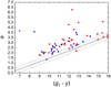 |
Fig. 1 a versus (𝑔1 – y) diagram for the 38 stars from our sample (red) and the 24 stars from the list of Mathys et al. (2024, blue) that have Gaia BP/RP spectra available. The normality line a = −2.16(8) + 0.363(8)(𝑔1 – y) is defined as in the classical ∆a photometric system. The dotted lines are the 95% prediction bands to select magnetic CP stars. |
3.2.2 ∆a photometry
∆a photometry is a powerful tool for investigating CP stars (Paunzen et al. 2005). It investigates the flux depression at 5200 Å, a spectral feature solely occurring in magnetic CP stars. The photometric system samples the depth of this feature by comparing the flux at the centre with those of the adjacent regions using bandwidths of 110–230 Å. The flux depression is caused by the line blanketing of Cr, Fe, and Si that is enhanced by a magnetic field (Kupka et al. 2003; Khan & Shulyak 2007). It is most significantly visible in magnetic CP stars. However, not all these objects show this flux depression, probably due to observational reasons (an unfavourable inclination) and the magnetic field characteristics (Paunzen et al. 2005). In addition, some (non- or only weakly magnetic) Am/CP1 and HgMn/CP3 stars also show detectable positive ∆a values but with much less significance.
We used the approach presented by Paunzen & Prišegen (2022), who used Gaia BP/RP spectra to synthesise ∆a photometry. They found a detection level of more than 85% for almost the entire investigated spectral range of the upper main sequence. 38 of our sample stars have BP/RP spectra available. According to Paunzen & Prišegen (2022), a ∆a value larger than 0.3 is significant. 31 sample stars fulfil this criterion (Table A.1), which is in line with the detection level of ~85% and is additional independent proof that these objects are bona fide magnetic CP stars. The remaining seven objects have no significant detectable flux depression at 5200 Å (which does not a priori exclude them from being Ap stars).
The ∆a values of our sample stars are listed in Table A.1, together with ∆a values for the 24 known ssrAp stars from Table 1 of Mathys et al. (2024) that also have BP/RP spectra available. The a versus (𝑔1 – y) diagram for all these objects is shown in Fig. 1. The ∆a values for the Mathys et al. (2024) stars were determined in the same way as described above.
3.3 Spectral classification
All available low-resolution spectra for our sample stars were downloaded from the LAMOST spectral archive2. Only spectra of sufficient signal-to-noise ratios (SNRs ≥ 20) were considered. As a result, spectra were downloaded for five sample stars.
Spectral classification was performed in the framework of the refined MK classification system following Gray & Garrison (1987, 1989a,b), Garrison & Gray (1994), and Gray & Corbally (2009). To derive a precise classification and identify peculiarities, the blue-violet (3800–4600 Å) spectral region was compared visually to, and overlaid with, MK standard star spectra, which were taken from the llbr18 collections available from R. O. Gray’s MKCLASS website3. Where appropriate, spectral types based on the Ca II K line strength (the k-line type) and the hydrogen-line profile (the h-line type) were determined (Osawa 1965; Gray & Corbally 2009). As the metallic lines of most Ap stars are so peculiar that they cannot be used for luminosity classification, luminosity types were based on the wings of the hydrogen lines (Gray & Corbally 2009).
An example of this process is illustrated in Fig. 2. All stars classified in this way turned out to be bona fide Ap stars, which is again independent proof of the effectiveness of the sample selection process. In addition, all spectra showed the characteristic 5200 Å depression.
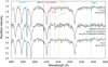 |
Fig. 2 Blue-violet region of the LAMOST spectrum of the Ap star Gala DR3 456836605925448448 = LAMOST J021027.46+551700.6 (middle spectrum), compared with two standard star spectra taken from the librl8_225 collection. Some prominent lines and blends relevant to the classification of Ap stars are identified. We note the peculiarly strong Cr II, Sr II, and Eu II features and the weak Ca II K line in the Ap star. |
4 Results
4.1 Basic parameters
Basic parameters of the final sample of 70 ssrAp stars identified in this study are listed in Table A.2. Positional information and magnitude in the G band were taken from Gala DR3 (Gaia Collaboration 2016, 2023; Babusiaux et al. 2023). All periods were derived using the Lomb-Scargle algorithm from PERANSO (Paunzen & Vanmunster 2016). Also indicated are the data sources the stars were retrieved from and remarks concerning the main photometric property the star was selected for.
Figure 3 presents the distribution of G magnitudes for our sample stars and the sample of ssrAp stars from Mathys et al. (2024), who present a census of the presently known ssrAp stars based on accurately determined period values or established period lower limits. The magnitude distribution of our sample stars has a broad maximum at G ~ 15 mag (mean magnitude G = 15.05 mag). Our work, therefore, extends the sample of known ssrAp stars to significantly lower magnitudes.
Figure 4 shows the distribution of rotation periods for the ssrAp stars from our sample and the sample of Mathys et al. (2024). For clarity, objects with period lower limits from the latter source are not included in the plot. It is obvious that our stars are situated at the shorter period end of the period distribution of ssrAp stars that shows a long tail petering out towards rotation periods of thousands of days and more. 42 of our sample stars have periods of 50 ≤ Prot ≤ 100 days; another 22 stars show periods of 100 < Prot ≤ 200 days. Only six stars show longer periods, with the longest-period object (Gaia DRЗ 456836605925448448) exhibiting a rotation period of Prot = 2551.7 days. This is to be expected: due to the limited time coverage, ZTF data are not well suited for the discovery of ssrAp stars with very long periods.
The phase plots for all our sample stars are provided in Fig. B.1, which is available on Zenodo4.
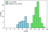 |
Fig. 3 Distribution of G magnitude brightness among our target star sample (green) and the sample of known ssrAp stars from Mathys et al. (2024, blue). |
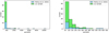 |
Fig. 4 Distribution of rotation periods among our target star sample (green) and the sample of known ssrAp stars from Mathys et al. (2024) (blue). The right panel provides a zoom-in on the period range from 50 to 650 days. |
4.2 Astrophysicаl parameters and Hertzsprung-Russell diagram
To locate the target stars in the HRD, we calibrated effective temperature (Teff) and surface gravity (log 𝑔) using the calibration published by Paunzen (2024). The latter is based on astrophysical parameters automatically determined by four independent methods using photometric and spectroscopic data. The paper presents a statistical analysis comparing the Teff and log 𝑔 from high-resolution spectroscopy and the sources correcting for offsets.
Table A.1 presents the mean values and their errors. The mean standard deviation of all Teff values is 10.4%, whereas it is 2.2% for log 𝑔, respectively. Figure 5 shows the HRD together with PARSEC isochrones (Bressan et al. 2012) for solar metallicity [Z] = 0.02 dex. As reported before (Hümmerich et al. 2020; Paunzen et al. 2021), the target stars are, with very few exceptions, grouped in the middle of the main sequence with ages older than 150 Myr.
Two stars are conspicuous by their outlying positions in the HRD and deserve special mention. HD 59435 is a well-established ssrAp star from the list of Mathys et al. (2024). It is a non-eclipsing double-lined spectroscopic binary (SB2) system consisting of a G8/K0 primary star and a cool SrCrEu (ssr)Ap secondary star (Wade et al. 1996). The presence of the giant star explains its outlying position in the HRD and is also clearly visible in the SED plot (Fig. 6, upper panel), which was created with the VO SED Analyzer (VOSA; Bayo et al. 2008), a browser-based online tool.
ZTF J021309.72+582827.7, on the other hand, is a ssrAp star from the new sample. Assuming that it is a main-sequence object, the derived temperature of ~6000 K would put this star at around a spectral type of F9, which is much too late for a classical Ap star. At this temperature, convection is expected to mix the stellar atmosphere, which effectively prevents the establishment of surface chemical peculiarities. Therefore, for main-sequence stars later than about F5, the typical Ap star peculiarities are not observed (Gray & Corbally 2009). There are, however, clear indications that ZTF J021309.72+582827.7 is indeed a chemically peculiar object. First, the ∆a value of 1.923 mag is a clear detection. Second, the amplitude of the photometric variations in r is much larger than the amplitude in 𝑔: while the star shows a ‘healthy’ amplitude of about 0.2 mag in the r band, the variations in the 𝑔 band are hardly noticeable with an amplitude of only about 0.05 mag. There are also slight indications of an antiphase pattern– when the star is brighter in r, it is fainter in 𝑔, and vice versa (cf. Fig. B.1 on Zenodo). The SED plot (Fig. 6, lower panel) indicates a strong infrared (IR) excess. Perhaps ZTF J021309.72+582827.7 is a binary star harbouring an Ap star and a cool component, possibly shrouded in dust. The strong IR excess could also point to a young stellar object; there is, however, no indication that the star is situated in a region of the sky with ongoing star formation. Only further spectroscopic investigations will be able to shed more light on this interesting object’s true nature.
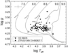 |
Fig. 5 HRD for our targets stars together with the PARSEC isochrones (Bressan et al. 2012) for the listed logarithmic ages and solar metallicity [Z] = 0.02 dex. In the left corner are the mean errors for the individual data shown. The two outliers (HD 59435 and ZTFJ021309.72+582827.7) are discussed in the text. |
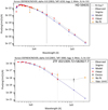 |
Fig. 6 SED plots for HD 59435 (upper panel) and ZTF J021309.72+582827.7 (lower panel), which were created with the VOSA tool. |
5 Conclusion
We have carried out a search for new ssrAp stars using data from the ZTF survey. Using suitable selection criteria based on known astrophysical and light curve properties of this group of stars and, where available, ∆a photometry and LAMOST spectra, we identified 70 new ssrAp stars. With a mean magnitude of G ~ 15 mag, we extend the sample of known ssrAp stars to significantly lower magnitudes. Our sample stars mostly exhibit rotation periods of between 50 and 200 days, with the longest period object having a period of Prot = 2551.7 days (Gala DR3 456836605925448448). We stress that because of the limited time span of the ZTF data, only Ap stars with rotation periods of up to about 3000 d could be unambiguously identified in our study which, therefore, is not suited for detecting Ap stars with very long rotation periods.
We have presented astrophysical parameters and a HRD for the sample of new ssrAp stars and the sample of known ssrAp stars with period determinations from Mathys et al. (2024). With only a few exceptions, all ssrAp stars are grouped in the middle of the main sequence with ages older than 150 Myr. Furthermore, ZTF J021309.72+582827.7 was identified as a possible binary star harbouring an Ap star and a cool component, possibly shrouded in dust, thus being a prime candidate for further detailed investigations.
With our work, we enlarge the sample of known ssrAp stars by about 150%, thereby paving the way for more in-depth statistical studies. Further investigations of our sample stars should include spectroscopic observations and magnetic field measurements.
Data availability
The phase plots for all our sample stars are made available under a Creative Commons Attribution license on Zenodo: doi:10.5281/zenodo.14225385.
Acknowledgements
We thank the referee, Dr. Gautier Mathys, for his valuable comments that improved the paper. We also thank Prof. Dr. Nikolay N. Samus for his help to identify the references pertaining to the initial denomination of the class of ACV variables. This study is based on observations obtained with the Samuel Oschin 48-inch Telescope at the Palomar Observatory as part of the Zwlcky Transient Facility project, which is supported by the National Science Foundation under Grant No. AST-1440341 and a collaboration including Caltech, IPAC, the Weizmann Institute for Science, the Oskar Klein Center at Stockholm University, the University of Maryland, the University of Washington, Deutsches Elektronen-Synchrotron and Humboldt University, Los Alamos National Laboratories, the TANGO Consortium of Taiwan, the University of Wisconsin at Milwaukee, and Lawrence Berkeley National Laboratories. Operations are conducted by COO, IPAC, and UW. This work also uses data from the Guoshoujing Telescope (the Large Sky Area Multi-Object Fiber Spectroscopic Telescope LAMOST), which is a National Major Scientific Project built by the Chinese Academy of Sciences. Funding for the project has been provided by the National Development and Reform Commission. LAMOST is operated and managed by the National Astronomical Observatories, Chinese Academy of Sciences. In addition, this work has made use of data from the European Space Agency (ESA) mission Gaia (https://www.cosmos.esa.int/gaia), processed by the Gaia Data Processing and Analysis Consortium (DPAC, https://www.cosmos.esa.int/web/gaia/dpac/consortium). Funding for the DPAC has been provided by national institutions, in particular the institutions participating in the Gaia Multilateral Agreement.
Appendix A Tables
Astrophysical parameters and synthetic Δa photometry for the merged samples of ssrAp stars and candidates.
Basic parameters for the newly identified sample of ssrAp stars and candidates.
References
- Anders, F., Khalatyan, A., Queiroz, A. B. A., et al. 2022, A&A, 658, A91 [NASA ADS] [CrossRef] [EDP Sciences] [Google Scholar]
- Andrae, R., Fouesneau, M., Creevey, O., et al. 2018, A&A, 616, A8 [NASA ADS] [CrossRef] [EDP Sciences] [Google Scholar]
- Babcock, H. W. 1958, ApJS, 3, 141 [Google Scholar]
- Babusiaux, C., Fabricius, C., Khanna, S., et al. 2023, A&A, 674, A32 [NASA ADS] [CrossRef] [EDP Sciences] [Google Scholar]
- Bagnulo, S., Fossati, L., Landstreet, J. D., & Izzo, C. 2015, A&A, 583, A115 [NASA ADS] [CrossRef] [EDP Sciences] [Google Scholar]
- Bauer-Fasching, B., Bernhard, K., Brändli, E., et al. 2024, A&A, 687, A211 [NASA ADS] [CrossRef] [EDP Sciences] [Google Scholar]
- Bayo, A., Rodrigo, C., Barrado Y Navascués, D., et al. 2008, A&A, 492, 277 [NASA ADS] [CrossRef] [EDP Sciences] [Google Scholar]
- Bellm, E. C., Kulkarni, S. R., Graham, M. J., et al. 2019, PASP, 131, 018002 [Google Scholar]
- Bernhard, K., Hümmerich, S., Otero, S., & Paunzen, E. 2015a, A&A, 581, A138 [NASA ADS] [CrossRef] [EDP Sciences] [Google Scholar]
- Bernhard, K., Hümmerich, S., & Paunzen, E. 2015b, Astron. Nachr., 336, 981 [NASA ADS] [CrossRef] [Google Scholar]
- Bernhard, K., Hümmerich, S., & Paunzen, E. 2020, MNRAS, 493, 3293 [NASA ADS] [CrossRef] [Google Scholar]
- Borra, E. F., & Landstreet, J. D. 1980, ApJS, 42, 421 [Google Scholar]
- Bressan, A., Marigo, P., Girardi, L., et al. 2012, MNRAS, 427, 127 [NASA ADS] [CrossRef] [Google Scholar]
- Chen, X., Wang, S., Deng, L., et al. 2020, ApJS, 249, 18 [NASA ADS] [CrossRef] [Google Scholar]
- Cui, X.-Q., Zhao, Y.-H., Chu, Y.-Q., et al. 2012, Res. Astron. Astrophys., 12, 1197 [Google Scholar]
- Faltová, N., Kallová, K., Prišegen, M., et al. 2021, A&A, 656, A125 [NASA ADS] [CrossRef] [EDP Sciences] [Google Scholar]
- Gaia Collaboration (Prusti, T., et al.) 2016, A&A, 595, A1 [NASA ADS] [CrossRef] [EDP Sciences] [Google Scholar]
- Gaia Collaboration (Vallenari, A., et al.) 2023, A&A, 674, A1 [NASA ADS] [CrossRef] [EDP Sciences] [Google Scholar]
- Garrison, R. F., & Gray, R. O. 1994, AJ, 107, 1556 [NASA ADS] [CrossRef] [Google Scholar]
- Gray, R. O., & Corbally, J., C. 2009, Stellar Spectral Classification (Princeton: Princeton University Press) [Google Scholar]
- Gray, R. O., & Garrison, R. F. 1987, ApJS, 65, 581 [NASA ADS] [CrossRef] [Google Scholar]
- Gray, R. O., & Garrison, R. F. 1989a, ApJS, 69, 301 [Google Scholar]
- Gray, R. O., & Garrison, R. F. 1989b, ApJS, 70, 623 [NASA ADS] [CrossRef] [Google Scholar]
- Gröbel, R., Hümmerich, S., Paunzen, E., & Bernhard, K. 2017, New A, 50, 104 [CrossRef] [Google Scholar]
- Hall, D. S. 1976, IAU Colloq., 29, 287 [NASA ADS] [Google Scholar]
- Hou, W., Luo, A., Yang, H., et al. 2015, MNRAS, 449, 1401 [CrossRef] [Google Scholar]
- Hubrig, S., North, P., & Schöller, M. 2007, Astron. Nachr., 328, 475 [NASA ADS] [CrossRef] [Google Scholar]
- Hümmerich, S., Paunzen, E., & Bernhard, K. 2016, AJ, 152, 104 [CrossRef] [Google Scholar]
- Hümmerich, S., Mikulášek, Z., Paunzen, E., et al. 2018, A&A, 619, A98 [NASA ADS] [CrossRef] [EDP Sciences] [Google Scholar]
- Hümmerich, S., Paunzen, E., & Bernhard, K. 2020, A&A, 640, A40 [NASA ADS] [CrossRef] [EDP Sciences] [Google Scholar]
- Hümmerich, S., Paunzen, E., & Bernhard, K. 2022, MNRAS, 517, 4229 [CrossRef] [Google Scholar]
- International Astronomical Union (Pecker, J.-C., et al.) 1966, Transactions of the International Astronomical Union, Volume XIIB, Proceedings of the Twelfth General Assembly, 12, 269 [Google Scholar]
- Jagelka, M., Mikulášek, Z., Hümmerich, S., & Paunzen, E. 2019, A&A, 622, A199 [NASA ADS] [CrossRef] [EDP Sciences] [Google Scholar]
- Khan, S. A., & Shulyak, D. V. 2007, A&A, 469, 1083 [NASA ADS] [CrossRef] [EDP Sciences] [Google Scholar]
- Kochukhov, O., & Bagnulo, S. 2006, A&A, 450, 763 [NASA ADS] [CrossRef] [EDP Sciences] [Google Scholar]
- Krtička, J., Mikulášek, Z., Lüftinger, T., et al. 2012, A&A, 537, A14 [NASA ADS] [CrossRef] [EDP Sciences] [Google Scholar]
- Kukarkin, B. V., Parenago, P. P., Efremow, Y. I., & Kholopov, P. N. 1958, General Catalogue of Variable Stars, 2nd edn. (Moscow: Academy of Sciences Publishing House), I & II [Google Scholar]
- Kupka, F., Paunzen, E., & Maitzen, H. M. 2003, MNRAS, 341, 849 [NASA ADS] [CrossRef] [Google Scholar]
- Labadie-Bartz, J., Hümmerich, S., Bernhard, K., Paunzen, E., & Shultz, M. E. 2023, A&A, 676, A55 [NASA ADS] [CrossRef] [EDP Sciences] [Google Scholar]
- Masci, F. J., Laher, R. R., Rusholme, B., et al. 2019, PASP, 131, 018003 [Google Scholar]
- Mathys, G. 1991, A&AS, 89, 121 [NASA ADS] [Google Scholar]
- Mathys, G. 2020, in Stellar Magnetism: A Workshop in Honour of the Career and Contributions of John D. Landstreet, eds. G. Wade, E. Alecian, D. Bohlender, & A. Sigut, 11, 35 [NASA ADS] [Google Scholar]
- Mathys, G., Hubrig, S., Landstreet, J. D., Lanz, T., & Manfroid, J. 1997, A&AS, 123, 353 [NASA ADS] [CrossRef] [EDP Sciences] [Google Scholar]
- Mathys, G., Romanyuk, I.I., Hubrig, S., et al. 2019, A&A, 624, A32 [NASA ADS] [CrossRef] [EDP Sciences] [Google Scholar]
- Mathys, G., Khalack, V., & Landstreet, J. D. 2020a, A&A, 636, A6 [Google Scholar]
- Mathys, G., Kurtz, D. W., & Holdsworth, D. L. 2020b, A&A, 639, A31 [NASA ADS] [CrossRef] [EDP Sciences] [Google Scholar]
- Mathys, G., Kurtz, D. W., & Holdsworth, D. L. 2022, A&A, 660, A70 [NASA ADS] [CrossRef] [EDP Sciences] [Google Scholar]
- Mathys, G., Holdsworth, D. L., & Kurtz, D. W. 2024, A&A, 683, A227 [NASA ADS] [CrossRef] [EDP Sciences] [Google Scholar]
- Mikulášek, M., Zverko, J., Krticka, J., et al. 2007, in Physics of Magnetic Stars, eds. I. I. Romanyuk, D. O. Kudryavtsev, O. M. Neizvestnaya, & V. M. Shapoval (USA: ASP Books), 300 [Google Scholar]
- Mikulášek, Z., Semenko, E., Paunzen, E., et al. 2022, A&A, 668, A159 [NASA ADS] [CrossRef] [EDP Sciences] [Google Scholar]
- Molnar, M. R. 1973, ApJ, 179, 527 [NASA ADS] [CrossRef] [Google Scholar]
- Molnar, M. R. 1975, AJ, 80, 137 [NASA ADS] [CrossRef] [Google Scholar]
- Morgan, W. W. 1933, ApJ, 77, 330 [NASA ADS] [CrossRef] [Google Scholar]
- Netopil, M., Paunzen, E., Hümmerich, S., & Bernhard, K. 2017, MNRAS, 468, 2745 [NASA ADS] [CrossRef] [Google Scholar]
- Osawa, K. 1965, Ann. Tokyo Astron. Observ., 9, 121 [Google Scholar]
- Paunzen, E. 2024, A&A, 683, L7 [NASA ADS] [CrossRef] [EDP Sciences] [Google Scholar]
- Paunzen, E., & Maitzen, H. M. 1998, A&AS, 133, 1 [NASA ADS] [CrossRef] [EDP Sciences] [Google Scholar]
- Paunzen, E., & Prišegen, M. 2022, A&A, 667, L10 [NASA ADS] [CrossRef] [EDP Sciences] [Google Scholar]
- Paunzen, E., & Vanmunster, T. 2016, Astron. Nachr., 337, 239 [NASA ADS] [CrossRef] [Google Scholar]
- Paunzen, E., Stütz, C., & Maitzen, H. M. 2005, A&A, 441, 631 [NASA ADS] [CrossRef] [EDP Sciences] [Google Scholar]
- Paunzen, E., Supíková, J., Bernhard, K., Hümmerich, S., & Prišegen, M. 2021, MNRAS, 504, 3758 [NASA ADS] [CrossRef] [Google Scholar]
- Phillips, A., Kochanek, C. S., Jayasinghe, T., et al. 2024, MNRAS, 527, 5588 [Google Scholar]
- Preston, G. W. 1974, ARA&A, 12, 257 [Google Scholar]
- Qin, L., Luo, A. L., Hou, W., et al. 2019, ApJS, 242, 13 [NASA ADS] [CrossRef] [Google Scholar]
- Renson, P., & Manfroid, J. 2009, A&A, 498, 961 [NASA ADS] [CrossRef] [EDP Sciences] [Google Scholar]
- Romanyuk, I. I., Semenko, E. A., & Kudryavtsev, D. O. 2014, Astrophys. Bull., 69, 427 [NASA ADS] [CrossRef] [Google Scholar]
- Romanyuk, I. I., Semenko, E. A., & Kudryavtsev, D. O. 2015, Astrophys. Bull., 70, 444 [NASA ADS] [CrossRef] [Google Scholar]
- Romanyuk, I. I., Semenko, E. A., Kudryavtsev, D. O., & Moiseevaa, A. V. 2016, Astrophys. Bull., 71, 302 [NASA ADS] [CrossRef] [Google Scholar]
- Romanyuk, I. I., Semenko, E. A., Kudryavtsev, D. O., Moiseeva, A. V., & Yakunin, I. A. 2017, Astrophys. Bull., 72, 391 [NASA ADS] [CrossRef] [Google Scholar]
- Romanyuk, I. I., Semenko, E. A., Moiseeva, A. V., Kudryavtsev, D. O., & Yakunin, I. A. 2018, Astrophys. Bull., 73, 178 [NASA ADS] [CrossRef] [Google Scholar]
- Romanyuk, I. I., Moiseeva, A. V., Semenko, E. A., Kudryavtsev, D. O., & Yakunin, I. A. 2020, Astrophys. Bull., 75, 294 [NASA ADS] [CrossRef] [Google Scholar]
- Romanyuk, I. I., Moiseeva, A. V., Semenko, E. A., Kudryavtsev, D. O., & Yakunin, I. A. 2022a, Astrophys. Bull., 77, 94 [NASA ADS] [CrossRef] [Google Scholar]
- Romanyuk, I. I., Moiseeva, A. V., Semenko, E. A., Yakunin, I. A., & Kudryavtsev, D. O. 2022b, Astrophys. Bull., 77, 271 [NASA ADS] [CrossRef] [Google Scholar]
- Romanyuk, I. I., Moiseeva, A. V., Semenko, E. A., Yakunin, I. A., & Kudryavtsev, D. O. 2023, Astrophys. Bull., 78, 567 [NASA ADS] [CrossRef] [Google Scholar]
- Samus, N. N., Kazarovets, E. V., Durlevich, O. V., Kireeva, N. N., & Pastukhova, E. N. 2017, Astron. Rep., 61, 80 [Google Scholar]
- Shang, L.-H., Luo, A. L., Wang, L., et al. 2022, ApJS, 259, 63 [NASA ADS] [CrossRef] [Google Scholar]
- Shi, F., Zhang, H., Fu, J., Kurtz, D., & Xiang, M. 2023, ApJ, 943, 147 [NASA ADS] [CrossRef] [Google Scholar]
- Sikora, J., David-Uraz, A., Chowdhury, S., et al. 2019, MNRAS, 487, 4695 [Google Scholar]
- Soszyński, I., Skowron, D. M., Udalski, A., et al. 2024, ApJ, 965, L17 [CrossRef] [Google Scholar]
- Stibbs, D. W. N. 1950, MNRAS, 110, 395 [Google Scholar]
- Tian, X.-m., Wang, Z.-h., Zhu, L.-y., & Yang, X.-L. 2023, ApJS, 266, 14 [NASA ADS] [CrossRef] [Google Scholar]
- Wade, G. A., North, P., Mathys, G., & Hubrig, S. 1996, A&A, 314, 491 [NASA ADS] [Google Scholar]
- Wolff, S. C., & Wolff, R. J. 1971, AJ, 76, 422 [NASA ADS] [CrossRef] [Google Scholar]
- Zhao, G., Zhao, Y.-H., Chu, Y.-Q., Jing, Y.-P., & Deng, L.-C. 2012, Res. Astron. Astrophys., 12, 723 [NASA ADS] [CrossRef] [Google Scholar]
All Tables
Astrophysical parameters and synthetic Δa photometry for the merged samples of ssrAp stars and candidates.
Basic parameters for the newly identified sample of ssrAp stars and candidates.
All Figures
|
Fig. 1 a versus (𝑔1 – y) diagram for the 38 stars from our sample (red) and the 24 stars from the list of Mathys et al. (2024, blue) that have Gaia BP/RP spectra available. The normality line a = −2.16(8) + 0.363(8)(𝑔1 – y) is defined as in the classical ∆a photometric system. The dotted lines are the 95% prediction bands to select magnetic CP stars. |
| In the text | |
|
Fig. 2 Blue-violet region of the LAMOST spectrum of the Ap star Gala DR3 456836605925448448 = LAMOST J021027.46+551700.6 (middle spectrum), compared with two standard star spectra taken from the librl8_225 collection. Some prominent lines and blends relevant to the classification of Ap stars are identified. We note the peculiarly strong Cr II, Sr II, and Eu II features and the weak Ca II K line in the Ap star. |
| In the text | |
|
Fig. 3 Distribution of G magnitude brightness among our target star sample (green) and the sample of known ssrAp stars from Mathys et al. (2024, blue). |
| In the text | |
|
Fig. 4 Distribution of rotation periods among our target star sample (green) and the sample of known ssrAp stars from Mathys et al. (2024) (blue). The right panel provides a zoom-in on the period range from 50 to 650 days. |
| In the text | |
|
Fig. 5 HRD for our targets stars together with the PARSEC isochrones (Bressan et al. 2012) for the listed logarithmic ages and solar metallicity [Z] = 0.02 dex. In the left corner are the mean errors for the individual data shown. The two outliers (HD 59435 and ZTFJ021309.72+582827.7) are discussed in the text. |
| In the text | |
|
Fig. 6 SED plots for HD 59435 (upper panel) and ZTF J021309.72+582827.7 (lower panel), which were created with the VOSA tool. |
| In the text | |
Current usage metrics show cumulative count of Article Views (full-text article views including HTML views, PDF and ePub downloads, according to the available data) and Abstracts Views on Vision4Press platform.
Data correspond to usage on the plateform after 2015. The current usage metrics is available 48-96 hours after online publication and is updated daily on week days.
Initial download of the metrics may take a while.