| Issue |
A&A
Volume 692, December 2024
|
|
|---|---|---|
| Article Number | A62 | |
| Number of page(s) | 11 | |
| Section | Planets, planetary systems, and small bodies | |
| DOI | https://doi.org/10.1051/0004-6361/202451407 | |
| Published online | 03 December 2024 | |
Surface dynamics of small fast-rotating asteroids: Analysis of possible regolith on asteroid 2016 HO3
1
Research Centre for Deep Space Explorations | Department of Land Surveying and Geo-Informatics, The Hong Kong Polytechnic University,
Hung Hom,
Kowloon,
Hong Kong
2
Department of Earth and Planetary Sciences, The University of Texas at Austin,
2305 Speedway Stop C1160,
Austin,
TX
78712-1692,
USA
3
Oden Institute for Computational Engineering and Sciences, The University of Texas at Austin,
201 E 24th St.,
Austin,
TX
78712,
USA
★ Corresponding author; This email address is being protected from spambots. You need JavaScript enabled to view it.
Received:
6
July
2024
Accepted:
23
October
2024
Abstract
The Chinese Tianwen-2 mission is planned to explore and sample the near-Earth asteroid 2016 HO3, also named 469219 Kamo’oalewa. This paper intends to answer the question of whether 2016 HO3 has any regolith. A 3D model of an irregular shape was reconstructed from light curve data of 2016 HO3, with simulated impact craters embedded on its surface. We used numerical simulations to calculate the acceleration from gravity, fast rotation, and the van der Waals cohesive force. We found that the poles have a higher chance of hosting regolith, and the regolith may also rest on the walls of craters that face toward the rotation axis, making them potential sample collection sites. On the surface of 2016 HO3, the van der Waals force is strong enough to hold particles smaller than several centimeters against centrifugal force. Furthermore, we compare a pair of transient processes: thermal fatigue, which generates small particles, and micro-impacts, which remove the surface mass. Thermal fatigue is at least comparable to, and perhaps more efficient than, micro-impacts for 2016 HO3. Therefore, it is highly possible that regolith exists on the surface of 2016 HO3.
Key words: minor planets, asteroids: general / minor planets, asteroids: individual: 469219 Kamo’oalewa / minor planets, asteroids: individual: 2016 HO3
© The Authors 2024
 Open Access article, published by EDP Sciences, under the terms of the Creative Commons Attribution License (https://creativecommons.org/licenses/by/4.0), which permits unrestricted use, distribution, and reproduction in any medium, provided the original work is properly cited.
This article is published in open access under the Subscribe to Open model. This email address is being protected from spambots. You need JavaScript enabled to view it. to support open access publication.
1 Introduction
Asteroids are valuable sources of information about the evolution of the Solar System and may contain clues to help reveal the formation of terrestrial planets and the origins of life. Meanwhile, the term asteroid has been used to describe a wide range of small bodies, from the 2 m near-Earth asteroid (NEA) 2015 TC25 (Reddy et al. 2016) to the differentiated asteroid 4 Vesta with a mean diameter of 525 km (Russell et al. 2012). Here we focus on small fast-rotating asteroids (SFRAs), with the example of 2016 HO3 (also named 469219 Kamo’oalewa) (de la Fuente Marcos & de la Fuente Marcos 2016). 2016 HO3 is one of the most stable of the seven quasi-satellites of the Earth (Reddy et al. 2017). Recently, spectrum and orbital dynamics studies have suggested that 2016 HO3 was formed from lunar ejecta (Sharkey et al. 2021; Castro-Cisneros et al. 2023). 2016 HO3 was selected as the first target for exploration and sampling by China’s Tianwen-2 mission, which is scheduled to be launched in 2025 (Li et al. 2024). Thus, 2016 HO3 will be the first SFRA and the smallest asteroid that has ever been studied by space missions (Veverka et al. 2001; Yano et al. 2006; Russell et al. 2012; Sierks et al. 2015; Park et al. 2016; Müller et al. 2017; Walsh et al. 2019). The basic information of 2016 HO3 is listed with some other explored asteroids in Table 1.
2016 HO3 spins with a period of 0.467 ± 0.008 h (Warner et al. 2021), which means that the centrifugal acceleration is stronger than the gravitational acceleration at most areas except the poles (Harris 1996; Pravec & Harris 2000). If a bulk density of 2700 kg/m3 is assumed, the rotation period threshold to bond materials gravitationally is about 2.0 h. In the present work, we define the term small fast-rotating asteroid (SFRA) as an asteroid with a size of ~300 m (Persson & Biele 2022) that rotates faster than the gravitational bonding threshold (fission failure) corresponding to its density. An internal coherent force is required for SFRAs to hold together, and the extremely fast-spinning small asteroids have even been considered bare rocks (Whiteley et al. 2002). Statistically, over two-thirds of the asteroids with absolute magnitude H > 20 (roughly equivalent to diameter < 100 m) rotate with periods significantly shorter than 2.0 h, and among all the larger asteroids, all but three rotate slower than 2.0 h per round (Hergenrother & Whiteley 2011). In addition to its unique orbit and origin of composition, the fast-spin feature also makes 2016 HO3 an interesting object to study by space mission, which will help in understanding the origin of SFRAs and the distinct difference in rotation period between asteroids smaller or larger than ~300 m. On the other hand, the fast-spin feature also raises challenges to the mission, in terms of attaching and sampling.
The question that we want to answer is whether 2016 HO3 has regolith. Although regolith has been found on 25143 Itokawa (Miyamoto et al. 2007; Tsuchiyama et al. 2011), 162173 Ryugu (Morota et al. 2020) and Bennu (DellaGiustina et al. 2019), there are no direct observations to support or rule out the existence of regolith on SFRAs. Fast rotators have been described as monolithic and regolithless (Whiteley et al. 2002). Some recent studies on 2016 HO3 (Li et al. 2023; Zhang et al. 2021) also suggested that its surface particles are likely to escape eventually. However, the effects of surface forces other than gravity and centrifugal force were not considered in those studies. For a typical SFRA, the outward accelerations of subcentimeter-sized grains can be balanced by van der Waals cohesive forces (Sánchez & Scheeres 2020; Scheeres et al. 2010). Li & Scheeres (2021) investigated possible regolith on the surface of 2016 HO3 with an ellipsoid model. They suggested that a layer of millimeter-sized to centimeter-sized grains can exist on the surface of 2016 HO3, and the required cohesion to bond such particles is less than 0.2 Pa. For reference, the considered “near-zero” cohesion on the subsurface of Bennu is approximately 0.2–20 Pa (Walsh et al. 2022) or <0.001 Pa (Lauretta et al. 2022), derived from numerical simulation or empirical relationships, respectively. While the surface dynamical environment of 2016 HO3 was presented in those studies, essential transient processes to generate and remove regoliths, such as thermal fatigue (Delbo et al. 2014) and impacts, have not been investigated for the SFRA scenario.
In this paper we present a dynamical model of 2016 HO3 considering gravity, rotation, and van der Waals forces with a shape model reconstructed from light curves and added crater features. Upon the shape and surface dynamical environment models, we further include the two most important transient processes, micro-impacts and thermal fatigue, which are generally destructive and constructive to the regolith, respectively. The motivation of the present work is twofold: to provide useful information for the upcoming missions and to develop a relatively unbiased theoretical model to compare with the future SFRAs’ observations. The paper is organized as follows. In Sect. 2 we describe our prediction of the shape of 2016 HO3 based on current observations and then analyze the stability and distribution of regolith on its surface for the general steady status. In Sect. 3 we compute and compare the regolith removal rate from micro-impacts and the production rate from thermal fatigue. Finally, the influence of assumptions, uncertainties, and implications for regolith existence on 2016 HO3 are discussed in Sect. 4.
Basic information of some asteroids and their moonlets as targets of space missions.
2 Shape and surface dynamical environment models of 2016 HO3
2.1 Shape model
2.1.1 Shape modeling of asteroid 2016 HO3 from light curves
By measuring the asteroid’s brightness (or magnitude) corresponding to its observed time, the light curves of the asteroid can be generated. The idea of deriving a 3D shape model of an asteroid from light-curve inversion is to find a shape model that generates light curves that closely match the observed light curves based on mathematic functions such as L = A𝑔, where L is the vector of the observed brightnesses, 𝑔 defines the facets of a convex polyhedron approximating the 3D shape model of the asteroid, and A is the reflectance that combines the light scattering on all the facets at an estimated surface albedo. By giving a set of light-curve observations, the optimal 3D shape model of the asteroid can be estimated through a least-squares solution (Kaasalainen et al. 2001).
Figure 1 shows examples of the light curves (top four rows) used to estimate the 3D shape model of asteroid 2016 HO3. In total, 15 light curves were used to derive a 3D shape model for 2016 HO3 (bottom row in Fig. 1). The root mean square error (RMSE) between the observed light curves and the model-derived light curves is 0.17, which indicates a relatively low precision for shape modeling from light-curve inversion. However, it should be noted that this is the shape modeling result from the available light curves for 2016 HO3. It may not represent the real shape model of 2016 HO3, but it can be used as a basis for the simulation analysis in this study.
To demonstrate the effect of different geometry, we built two models (shown in Fig. 2): a polyhedral approximated ellipsoid (Model A) and a reconstructed model based on our interpretation of available light curves (Model B) of 2016 HO3. The dimensions of Model B are 100 m × 81 m × 46 m. Figure 2c shows the bottom view of Model B. We assumed the asteroid rotates around the Z-axis. The lengths of the three axes of Model A were determined with the ratio a/b/c=1/0.4786/0.4786 (model I in Li & Scheeres 2021) to make its total volume equal to Model B. Numerically, we only needed to mesh the surface of models: 4483 vertices and 8963 triangles were used for Model A, and 2521 vertices and 5038 triangles were used for Model B.
2.1.2 Adding craters on the 3D shape model of 2016 HO3
Since large boulders on SFRAs are likely to escape (see explanation in Sect. 2.2), craters are the only type of additional features we added to the asteroid. We mainly focused on two features for crater simulation. Crater size-frequency distribution describes the relationship between the size and the amount that is commonly defined in the form N = cD−β, where N is the number of craters with size ≥ D, β mainly contributes to size distribution and varies depending on asteroids, and c determines the final amounts. Since we did not have close observations of asteroids as small as this size, we referenced the statistical results of asteroid (433) Eros (Ballouz et al. 2024) and Gaspra (Bottke et al. 2020) to decide these parameters. The shapes of craters, particularly depth to diameter ratio (d/D) were considered according to previous findings as well (Noguchi et al. 2021; Robinson et al. 2002).
We used self-developed in-house software to generate craters that satisfy the required parameters. By adjusting the physical properties of craters, we can customize the desired and appropriate shape models. Therefore, we imported the 3D shape model of 2016 HO3 derived from light curves as an initial input and determine physical parameters including c = 2× 10⁻⁴, β = −2.6, and d/D = 0.15 to mimic realistic crater distribution and morphological features. Figure 2 gives examples of the corresponding simulated shape models under different observing views. There are 12 craters ranging from 5 to 20 m and randomly distributed on the surface, including equatorial and polar regions. The areas of the triangle faces of Model A range from 1.4 to 3.9 m2, while Model B has a more uneven distribution of face areas, from 0.03 to 7.6 m2. This synthetic 3D shape model of 2016 HO3 is used for further analysis in this study.
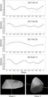 |
Fig. 1 Shape model of 2016 HO3 derived from light-curve inversion. Top four rows: examples of light curves (red dots) and the corresponding fits (solid lines) for estimating the shape of 2016 HO3. Bottom row: estimated 3D shape model of 2016 HO3. |
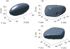 |
Fig. 2 Shape models, (a) Model A. (b) Top view of Model B. (c) Bottom view of Model B. |
2.2 Surface dynamical environment model
The gravitational and centrifugal accelerations are both proportional to the radius if we assume the asteroid is spherical and homogeneous in density. The net outward acceleration from gravity and rotation normal to the body surface is (Scheeres et al. 2010)
 (1)
(1)
where ω is the rotation speed, φ is the latitude, G is the gravitational constant, ρ is the bulk density, and R is the radius of the asteroid. In other words, if the shape ratio and density are fixed, the fission limit rotation period has the same value no matter how large the body is.
2.2.1 Gravitation
A nonspherical shape will make the direction of gravity acceleration not always point to its centroid, and the normal vector of the surface plane is not always parallel with the displacement from the centroid to the surface point of interest. Thus, a more irregular shape will distort Eq. (1) at certain locations, but the overall proportional relation to the asteroid size still stands. Equation (1) also shows how the limiting rotation period is determined and how it decreases proportional to the square root of the bulk density.
We adopted the method developed in Werner & Scheeres (1996) to calculate gravitational potential and acceleration, and we followed the modification in Yu & Baoyin (2015) to solve the singularity problem that happens when the field points are on the asteroid’s surface or interior. An asteroid with an irregular shape is approximated to a polyhedron with triangular faces. The basic idea of this method is to convert the volume-integral of gravity or gravitational potential to a surface integral, and further to line integrals plus surface integrals with analytical expressions via the Gauss divergence theorem. Written in the same form as in Yu & Baoyin (2015), the gravitational potential and its vectorial first-order gradient, gravitational acceleration, are
 (2)
(2)
 (3)
(3)
where re and rf are vectors from the interested field point to arbitrary points belonging to edge e and face f, respectively. Both Model A and Model B are regarded as a whole polyhedron with numerous faces in this work. In practice, we go over every face and edge on the model’s surface and pick a vertex point for each of them (e.g., restored in the first column) to calculate vectors re and rf. The edge dyad is defined as  , and the face dyad is defined as Ff = nfnf, where nf is the normal vector of plane f; nA, nB are unit normal vectors of two faces connected by edge e; and
  are the unit normal vectors of edge e, which lies in the face plane A and B, respectively. An instructive diagram of these vectors can be found in Fig. 7 in Werner & Scheeres (1996). Le and ωf are scalar integrals that can be expressed analytically:
 (4)
(4)
 (5)
(5)
Here a, b are the distances from the field point to the ends of the edge and el is the length of the edge; ri and ri (i = 1,2,3) are the vectors and distances from the field point to the vertices of the triangular face f. The indices of the vertices should be labeled in a way that the direction of the loop (1–2–3–1) points outward, defined by the right-hand rule.
As stated in the title of Werner & Scheeres (1996), the method originally applies only to “exterior” gravitation. Yu & Baoyin (2015) solved the singularity on the surface and interior of the polyhedron and rewrote Eqs. (2) and (3) as
 (6)
(6)
 (7)
(7)
where r is field point vector, and
 (8)
(8)
 (9)
(9)
Practically, we define field points on all centroids of triangle faces and implement Eq. (9) by setting Qf(r) = 0 to the corresponding face.
Adopting the above method, we investigated the surface environment of both the ellipsoid and the reconstructed model of 2016 HO3. First, the gravitational potential fields U and the vectorial gravitational accelerations ∇U at all centroids of the triangle faces were calculated. The calculation of gravitational fields runs relatively fast in a matrix format. It only took about 31 seconds to solve models A and B with a personal computer. The magnitudes of gravitational accelerations at the surface are shown in Fig. 3. The magnitudes of the two shapes are similar, from 2.0 to 2.6 µG. For Model A, because of the elongated shape, gravity is strongest around the rotation axis (Z-axis) and weakest at the endpoint of the max axis (X). This pattern also works for Model B, generally. Escape velocities υe are shown in Fig. 4. In the section of micro-impacts, all ejecta with υ > υe escapes the object.
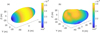 |
Fig. 3 Magnitudes of gravitational accelerations. |
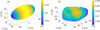 |
Fig. 4 Escape velocities |

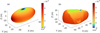 |
Fig. 5 Net gravitational and centrifugal acceleration normal to the surface faces, with measured rotation period of 0.467 h. Outward is defined as the positive direction. For both Model A and B, outward accelerations are shown in the warm color scale (yellow to red) and inward accelerations are shown in the cold color scale (green to blue). |
2.2.2 Rotation and simple friction
The magnitude of the centrifugal acceleration is calculated as
 (10)
(10)
where rx and ry are the x-axis and y-axis component of r, respectively. The direction of acen(r) is the projection of r on the plane normal to the Z-axis. The expression of the net acceleration of gravity and rotation in the numerical model is
 (11)
(11)
To determine whether a surface particle will be thrown out (fission failure), we calculated the normal component of the net acceleration, anet0 · nf, with the measured rotation period of 0.467 h (Warner et al. 2021); it is shown in Fig. 5. The net acceleration is dominated by rotation, and the result of Model A shows that the normal acceleration is only inward near the polar region, which is consistent with previous studies (Li et al. 2023; Li & Scheeres 2021; Zhang et al. 2021). However, Model B demonstrates some very interesting features about the craters. The strongest inward acceleration appears at the crater to the right of the north pole, with some distance. When the normal vector of a crater face, nf, generally points toward the rotation axis, the normal component of the centrifugal force presses the particle onto the surface instead of throwing the particle out. If the slope of the crater is steeper than the friction angle at that location, the regolith is able to rest in that area of the crater even without considering the normal component of cohesive forces. Therefore, in addition to polar regions, the inward faces of craters are also potential sites for sample collection, and the regolith there might be more stable against small disturbances since the normal force is enhanced by rotation.
Here we set the friction to µ = 1. The fission region, landslide region, and stable region are plotted in Fig. 6 in blue, green, and yellow, respectively. The particles in landslide regions are pushed toward the equator by the tangential part of centrifugal force and subsequently enter the fission region. The edges in Model A are not as regular because, in our numerical model, the field variables are assigned to every triangle face. The small disconnected yellow region in Model B again shows the role of craters in surface dynamics. Several faces in a crater in the southern hemisphere also form a stable region, which are not shown in Fig. 6.
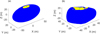 |
Fig. 6 Different dynamic regions resulting from the effects of gravity, centrifugal acceleration, and friction (coefficient µ = 1). The fission failure regions (where anet0 > 0) are labeled in blue, the landslide regions are in yellow, and the stable regions are in green.) |
2.2.3 van der Waals cohesive force
In addition to gravity and rotation, Scheeres et al. (2010) compared the effects of Coulomb friction, interior pressures, self-gravity, electrostatic forces, solar radiation pressure forces, and van der Waals forces. These forces have different dependent relations on the particle size, and the van der Waals force is the dominant force for particles smaller than 1 mm to 1 cm. The attractive van der Waals force (Castellanos 2005; Perko et al. 2001; Rognon et al. 2008) is computed as
 (12)
(12)
where A is the Hamaker coefficient in units of work (joules), t is the minimum interparticle distance between surfaces, d is the distance between particle surfaces, and r = rarb׀ (ra + rb) is defined as the reduced radius of the system. If we assign ra to 2016 HO3 and rb to a surface particle, we have r ≅ rb because ra ≫ rb. Following Scheeres et al. (2010) we set the distance term d to 0, and the force is only considered to be active when the bodies are in contact. By adopting Eq. (12), we assume all particles are perfect spheres with ideally smooth surfaces. Another possibility, that cohesive force is independent of particle size because of roughness (Persson & Biele 2022), is discussed in Sect 4.1. Our model only considers a scenario where a layer of separated particles rests directly on the surface of the polyhedral asteroid. As a result, the direction of the van der Waals forces on particles is normal to the faces and inward. The aim of this study is to analyze the dynamical environment of 2016 HO3’s surface and the existence of its regolith. Other properties and behaviors such as thickness and shear strength of the regolith are not included, but will be interesting topics once the existence of regolith on SFRAs is confirmed.
The effect of the van der Waals force is more important in the environment of space because in such an extreme environment the minimum distance between the materials, t, can be much closer than possible on Earth where atmospheric gases, water vapor, and relatively low temperatures allow the significant contamination of surfaces (Scheeres et al. 2010). Surface cleanliness, a nondimensional parameter, describes the level of such contamination,
 (13)
(13)
where Ω is the interparticle distance for lunar regolith and has the value of 1.5 × 10⁻¹⁰ m (Perko et al. 2001). Substituting Eq. (13),  and d = 0 into Eq. (12), we have
 (14)
(14)
where the Hamaker coefficient A = 4.3 × 10⁻²⁰ J (Perko et al. 2001). The value of the Hamaker coefficient is computed for lunar soil and might change on the surface of 2016 HO3 with different mineral assemblage and adsorbed medium. Now we have two free parameters, S and r. The surface cleanliness in the vacuum chamber (10−7 Pa) was estimated to be 0.58–0.77, from 294 K to 394 K (Perko et al. 2001), which was examined by both simulated lunar soil experiments (Nelson 1967; Nelson & Vey 1968) and actual lunar soil. The cohesive force Fc is proportional to the particle radius r, so that the cohesive acceleration follows the inverse square proportion: ac ∝ S2r−2. The net gravitational and centrifugal acceleration anet0 is independent of the particle’s size, while ac is independent of the asteroid’s size as long as ra ≫ rb. Therefore, with a fixed rotation speed, the van der Waals force becomes more important with the decrease in the asteroids’ size.
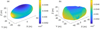 |
Fig. 7 Net outward normal acceleration from gravity, centrifugal force, and van der Waals forces. Under the choice of surface parameters, S = 0.1 and r = 1 mm, the van der Waals force dominates the surface dynamical environment. |
2.2.4 Distributions of surface particles
Now the van der Waals cohesive force is included. We first consider a modest surface cleanliness of S = 0.1, and assume the surface is covered with identical spherical grains with radii of 1 mm and the same densities as the asteroid. Hence, the cohesive acceleration ac is also a constant in this case, with a value of 0.0352 m s−2. Figure 7 shows the result of the combination of gravity, rotation, and the van der Waals force. To be consistent, outward is still the positive direction of acceleration. The cohesive force is the dominant effect this time. Dividing the net acceleration by the cohesive acceleration ac, the range of normalized acceleration is 0.98 to 1.00 for Model A and 0.98 to 1.01 for Model B. In Fig. 8, we keep the surface cleanliness to 0.1 and calculate the maximum radius that allows the particle to have a net inward normal acceleration. For the landslide and stable region shown in Fig. 6, this radius could be arbitrarily large to avoid fission failure, so we label those areas in red in Fig. 8. For both shape models, the maximum radius is smaller than several decimeters. Because ac ∝ S2r−2, the theoretical upper limit of particle radii is ten times larger than the result shown in Fig. 8, when S reaches its theoretical upper limit of 1.
For the calculation of landslide failure, several additional assumptions were made. Movements on the surface were considered quasi-static, which means we neglected the particles’ relative velocity to the surface. We also assumed a friction coefficient µ = 1 at all locations, giving a friction angle of 45°, and that the surface cleanliness was constant all over the surface.
Stable regions from the gravity and rotation results are special regions where the radii of particles are not limited. In practice, even in these special regions, the particle radius should still be smaller than the size of these regions themselves. At all the other regions, if a particle is not large enough to take off, but also not small enough to resist tangential acceleration, it will slide along the tangential direction that always points away from the rotation axis. Unless sliding into a proper crater, when a particle begins to slide, it is not likely to stop, and will finally end up flying into space because the tangential force increases with the rotation radius  . Figure 9 shows the maximum radii of stable particles with uniform surface cleanliness S = 0.1; we note that a stable particle is not related to the stable area. The special regions not applied maximum radii are labeled in red. For the other regions, the maximum stable radii are smaller than the maximum radii to avoid fission failure (see Fig. 8). It is interesting to note that in Model B, craters located close to the poles and/or having walls approximately facing toward the rotation axis can hold larger boulders up to about 1 m across.
To better understand the combined effects of different parameters, we further explored the space of the cleanliness, the grain size, and the coefficient of friction. For grains with a radius of 10 cm, 2016 HO3 could not be covered with such particles even if the cleanliness S = 1 everywhere, but down to 10s µm, the cohesive force is strong enough to retain such particles, even with a surface cleanliness as low as 0.001 if there is no other disturbance. Figure 10 shows the cumulative area fractions distributions regarding the maximum diameter of the stable particles for Model A (panel a) and Model B (panel b). For a certain small surface area, if the net effect of gravity, centrifugal force, and van der Waals force allows grains with a certain size to be stable at this area, then this area is added to the cumulative allowable area. It is not necessary that the area is actually covered by grains of such size. For a given area fraction between 0 and 1, the allowable grain size decreases proportionally with the decrease in cleanliness S, which is consistent with our previous analysis that cohesive acceleration is a function of S/r. A smaller µ also decreases the upper limit of grain size. Among cleanliness, the coefficient of friction, and shape models, cleanliness is the most important in order to determine the distribution of maximum possible grain size; the coefficient of friction also makes a difference. In terms of overall distribution, the effect of the shape model is negligible. However, as shown before, craters are important to dynamic environments locally and might be interesting spots for the upcoming space mission. The information of possible particle sizes on the surface of 2016 HO3 is important to the processes that generate and remove regolith (see next section).
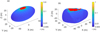 |
Fig. 8 Maximum particle radii to avoid fission failure when S = 0.1. Red shows both landslide and stable regions that are not applied to this non-fission maximum radius calculation. |
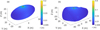 |
Fig. 9 Maximum radii of stable particles that will not slide under the coefficient of friction of µ = 1 and the cleanliness S = 0.1. |
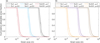 |
Fig. 10 Cumulative area distribution for the maximum grain diameters to avoid both landslide and fission failures. Panel a shows the results for shape Model A, and panel b shows the results for shape Model B. For each model, distributions for different parameter combinations, cleanliness S ∊ {1, 0.1, 0.01), and coefficient of friction µ ∊ {1, 0.5) are calculated. |
3 Transient processes
Thermal fatigue and meteoroid impacts are considered to be the two major regolith production and loss mechanisms (Li & Scheeres 2021; Hsu et al. 2022). Since impact ejecta velocities (Housen et al. 1979; Housen & Holsapple 2011) are typically much greater than the escape velocities of small asteroids, thermal fatigue (Delbo et al. 2014) is considered to be the dominant fragmentation process. Hsu et al. (2022) set the nominal thermal fragmentation rate of exposed rocks on airless bodies at 1 AU to be 5 × 10⁻¹¹ kg m−2 s−1, which is 100 times lower than the terrestrial value. To estimate the ejecta generation rate due to micro-impacts, Hsu et al. (2022) adopted interplanetary dust particle (IDP) density, impactor size of 100 µm, and an average impact speed of 17.9 km/s at 1 AU (Grün et al. 1985). With a mass ratio of ejecta to impactor (also called ejecta mass yield) of 1000 (Bernardoni et al. 2021), the calculated ejecta generation rate, 1–9 × 10⁻¹² kg m−2 s−1, matches the measured value around the Moon (Horányi et al. 2015). Considering the extremely low escape of 2016 HO3, υ ≈ 0.4 m/s, all ejecta will escape (see below). Therefore, a high-speed micro-impact is a purely destructive process for the surface mass of the asteroid. The question arises of whether it is enough to say that regolith production is faster than regolith loss in 2016 HO3. Due to its fast rotation and small size, this question is worth examining, as described below.
Mass loss rates per unit cross section of four different types of micro-impacts.
3.1 Micro-impacts
Micro-craters have been observed in returned asteroid samples. The surfaces of regolith returned from 25143 Itokawa contain craters with diameters of 100–200 nm and adhered objects (Nakamura et al. 2011). A large number of micro-craters and impact melt splashes have also been observed in particles from 162173 Ryugu (Matsumoto et al. 2024), and one investigated crater has a diameter of about 5 µm. However, the observed size of micro-craters might be biased by the relatively small size of particles we collected. Therefore, in this section we investigate the properties of micro-impactors and a single impact event for a typical NEA.
Constrained by Infrared Astronomical Satellite (IRAS) observations of thermal emission, about 90% of the observed mid-infrared emission is produced by particles from Jupiter-family comets (JFCs), and the present mass of the inner zodiacal cloud at <5 AU is mainly in D = 100–200 µm (Nesvorný et al. 2010). Thus, it is worth noting that the micro-impacts considered in this section are much smaller in scale than the impacts that create the craters on Model B in Sect. 2. For a particle in the zodiacal cloud, its average intrinsic impact probability on a circular cross section of radius 1 km per year for a typical NEA is p0 = 9.5 × 10⁻¹⁸ (Delbo et al. 2014). The next step is to find the total mass (number of meteoroids) of the zodiacal cloud. Nesvorný et al. (2010) estimated that with ρ = 2 g cm−3 and D = 200 µm, the total mass of the zodiacal cloud (mZODY) is 5.2 × 10¹⁶ kg. The total mass estimation also contains uncertainties from particle size and density; for example, if ρ = 1 g cm−3 or D = 100 µm, they calculated that mZODY = 2.6 × 10¹⁶ kg. We assume 1 g cm−3 for JFCs, so that mZODY = 1.3× 10¹⁶ kg for D = 100 µm, and mZODY = 2.6 × 10¹⁶ kg for D = 200 µm.
Next, we move to a single impact event. We adopted a point-source scaling model from Housen & Holsapple (2011). Such high-speed impacts to low-gravity targets belong to the strength regime, so we selected two patterns, C2 and C8 in Housen & Holsapple (2011). The results are shown in Fig. 11. In all four ejecta velocity distributions, the lowest velocities already exceed the escape velocity of 2016 HO3. Two solid curves show cases of rock target (black) and sand target (red) with impactor of D = 100 µm. Two dashed curves show cases with impactors of D = 200 µm. The diameters of craters range from 1.8 to 6.4 mm. Because all ejecta mass escapes, the mass loss per impact is doubled in D = 200 µm cases compared to D = 100 µm cases, with respect to the same target materials.
Combining the impact probability, number of meteoroids, mZODY, and ejecta distributions, the mass loss rates per square meter per second are computed and shown in Table 2. Those four values generally cover a range of mass loss rates due to micro-impacts, 1.46–7.58 × 10⁻¹² kg m−2 s−1. This range is close to the range of 1–9 × 10⁻¹² kg m−2 s−1 given in Hsu et al. (2022), though the physical aspects are different in these two scenarios.
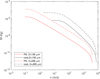 |
Fig. 11 Mass of ejecta with velocities > υ for four individual micro-impact events, and the impact velocity is always 15 km/s. The two red lines show impacts on perlite–sand mixture (PS) with high porosity (ϕ = 0.6), and the black lines show impacts on rock. Spherical impactors with diameters of 100 µm and 200 µm are shown as solid and dashed lines, respectively. |
3.2 Thermal fatigue
Thermal fatigue is considered a purely constructive process to produce regolith with no subsequent ejection (Delbo et al. 2014; Hsu et al. 2022), but also as a driving mechanism for in situ disaggregation and exfoliation on Bennu (Molaro et al. 2020). The short rotation period of 2016 HO3 of 0.467 h is also an important characteristic in terms of thermal fatigue. Compared with slower rotators, 2016 HO3 should have smaller diurnal temperature excursion, but also experience more thermal cycles. These two differences act against each other. In this section we adopt the methodology of Delbo et al. (2014) to analyze the regolith production on the surface of 2016 HO3 due to thermal fatigue. The method is briefly introduced in three parts: 1) thermal model, 2) macroscopic stress field, and 3) macroscopic stress field and fatigue crack growth.
First, we also adopted the same thermal model (Spencer et al. 1989) as Delbo et al. (2014) did to solve a one-dimensional heat diffusion problem, and we calculated the temperature profile for 16 skin depths (penetration depth of the diurnal thermal wave) from the surface. The skin depth is  , where κ is thermal conductivity, ρ is the density, c is the heat capacity, and ω is the rotation speed. Meanwhile, the amplitude and the lag of diurnal thermal wave is controlled by thermal inertia,
  . For example, ls = 1.27 cm and Γ = 640 J m−2 s−0.5 K−1 for carbonaceous chondrite (CC). Since ls is much smaller than the size of 2016 HO3, a 1D plane is not a bad approximation, but spherical or more general geometry simulations are expected in future work to investigate heat diffusion in angular directions. We simplified the perihelion distance of 2016 HO3 to be 1 AU, and the resulting temperature excursion for carbonaceous chondrite is 33.5 °C, lower than the value for asteroids with a longer rotation period presented in Delbo et al. (2014). The sub-solar temperature is 393.5 K, and the constant bottom boundary temperature is 295.0 K.
Next, to compute the required macroscopic stress field, we used the analytical solution (Capek & Vokrouhlický 2010), which was also adopted in Delbo et al. (2014). The thermal stress fields of three sizes of spherical particles were calculated, with diameters d = 1 cm, d = 2 cm, and d = 5 cm. Here we faced a problem of inconsistency in boundary conditions. With our best knowledge of the analytical solution (Capek & Vokrouhlický 2010), the result begins to diverge when the radius of the particle is much greater than the skin depth ls. Thus, we could not directly calculate the whole stress field of 2016 HO3 as an intact body with the analytical solution. Under this limit, the bottom boundary of a small particle is not the corresponding Dirichlet boundary in the 1D model, but the lower hemisphere is considered to directly radiate to the ambient space. Though this will introduce a system error, its final effect on the survival time of rocks is still limited.
Finally, we come to the microscopic stress field of inclusions and the fatigue crack growth mode. Recent spectrum and orbital dynamic studies suggested the lunar origin of 2016 HO3 (Sharkey et al. 2021; Castro-Cisneros et al. 2023), and a more recent orbital dynamic study (Jiao et al. 2024) even located the source at the Giordano Bruno crater. Therefore, in addition to calculating the survival time for carbonaceous and ordinary chondrite (OC) with the properties listed in Delbo et al. (2014), we also chose norite as a simulant of lunar crust material for the thermal fatigue model. Table 3 shows the properties of the norite used in the model. Unlike CC and OC, the microscopic stress field is not considered for norite. Thus, the time required to break norite is likely to be overestimated in the present study. For the geometric parameters in the crack growth model, we adopted the parameter set of disks (Glinka & Shen 1991) as an approximation of spheres. The times required to break CC, OC, and norite particles in diameters of 1 cm, 2 cm, and 5 cm are shown in Fig. 12. The error bars show that the uncertainties stem from 30% variations of thermal conductivity and bulk and shear moduli. The survival times of CC and OC particles are relatively close to Fig. 1 in Delbo et al. (2014), which is consistent with our previous qualitative analysis of smaller temperature excursion but more cycles.
Default values of physical properties of noгite.
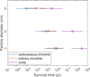 |
Fig. 12 Time required to break rocks on 2016 HO3. Blue: carbonaceous chondrite; orange: ordinary chondrite; and purple: norite. The symbols for ordinary chondrite have been manually shifted slightly upward to show the uncertainty bars more clearly. |
3.3 Combined results
In this section we give a final analysis of the existence of regolith on the surface of 2016 HO3 with the combination of our result on its dynamical environment and the two transient processes. First, we estimate that the cross section for impact is 0.25 times the total area of Model B, Across = 0.25 × AModel B = 4496 m2, so the impact probability of one meteoroid on the cross section of 2016 HO3 is  . Multiplying the mass loss rate per unit area in Table 2, the mass loss rate due to micro-impacts has a range of 0.21–1.1 kg/yr.
Then we consider the thermal fatigue of a layer of particles on the surface with diameters of 1, 2, and 5 cm. According to the distribution analysis in Sect. 2.2.4, this assumption of sizes is feasible when the cleanliness S ≥ 0.1. The regolith production rates are calculated by the mass of the one-particle layers divided by the break-up time computed in Sect. 3.2. The question arises of why we assume that regolith exists on the surface as an initial condition. First, the breakup times of the three cases are the first-order approximations of regolith production on any actual surface conditions of 2016 HO3. The range of possible scenarios could be from a bare rock without any regolith to a layered regolith of mixed particles with different sizes. Second, these cases also represent a potential transient or balanced state of the grain distribution of the surface since the initial condition of regolith thickness and particle size distribution of the surface is currently unavailable. Since the thermal fatigue process is not significantly affected by the gravity of the object, we decouple the value of the density from Sect. 2 and choose the density of CC, OC, and norite along with other physical properties. The result of the regolith production rate from thermal fatigue compared to the mass loss rate from micro-impacts is shown in Fig. 13. The error bars also show 30% relative uncertainty in the values of thermal conductivity and moduli. Compared with the regolith loss rate of ~0.2–1 kg/yr, the regolith production rate disperses more widely with regard to different materials and particle diameters. For CC and OC, thermal fatigue is more powerful in all cases except in 1 cm CC, which also lies inside the range of mass loss rate. In Fig. 13c, the regolith production rate of the norite surface is lower than the regolith loss for particle diameters of 1 and 2 cm, but higher when d = 5 cm. The production rate of norite regolith might be underestimated by not including the effect of its inclusion structure. To summarize, we predict that regolith is highly likely to exist on the surface of 2016 HO3, with considerations of a variety of possibilities of dynamic environment, types of micro-impacts, and surface materials.
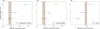 |
Fig. 13 Comparison of the regolith loss rate from micro-impacts (brown shaded area) and the regolith production rate from thermal fatigue. Surface materials are set to be (a) carbonaceous chondrite, (b) ordinary chondrite, and (c) norite. |
4 Discussion
4.1 Simplifications and assumptions
For simplicity, we used a constant density and assumed zero porosity for the whole body of 2016 HO3, which we describe in Sect. 2. However, it is worth noting that although short rotation periods are indicative of intrinsic strength in asteroids, it does not necessarily rule out the porosity of small fast-rotating asteroids. As Whiteley et al. (2002) hypothesized, SFRAs are representative of the building blocks of the rubble pile asteroids and also derived from fragmentation of already previous generation of rubble piles. Cohesive forces could form in previous generations of rubble piles and act as intrinsic strength to counter the centrifugal force later in SFRAs. Moreover, if all SFRAs with sizes up to ~300 m are monoliths, high-density monoliths with similar sizes should be included in rubble-pile asteroids such as Itokawa, Ryugu, and Bennu, but there is not any direct observational support for that yet. Adding bulk porosity decreases the strength of the gravity field, but also provides pores to trap regolith from thermal fatigue or impact shock. Moreover, because thermal conductivity decreases exponentially with the increase in porosity (Henke et al. 2012), both skin depth and thermal inertia decrease with the increase in porosity, and consequently the effect of thermal fatigue penetrates to a shallower level, but is also stronger within its effective depth.
In Sect. 2.2, we assume that all surface particles are perfect spheres, and the surfaces of 2016 HO3 and all particles are smooth. However, recent studies showed that both shape (Sanchez et al. 2023) and surface roughness (Persson & Biele 2022) affect the magnitude of the van der Waals force between an asteroid’s surface and particles. Persson & Biele (2022) suggested that surface roughness results in an interaction force that is independent of the size of the particles, in contrast to the linear size dependency in Eq. (12). They estimated van der Waals pull-off forces for meteorite particles of order 0.3–2 nN. In Fig. 14 we show the distribution of maximum radii of stable particles, with cohesive force F = 1 nN and the coefficient of friction µ = 1. Although the van der Waals force is independent of the particle size in this case, the outward centrifugal force is still dependent on it. Compared with Fig. 9, the maximum particle sizes decrease ~100 times. Neither of the relationships based on perfect spheres (Perko et al. 2001) or surface roughness (Persson & Biele 2022) has been directly tested by experiments, so the Tianwen-2 mission will also be a good opportunity to test which relationship better describes the reality, with the consideration of other important processes.
Another important simplification is that we neglect orbital characteristics, such as eccentricity and inclination, obliquity, and latitude differences. In Sect. 3.2 the survival time is only calculated for the equator area, and the sunlight is always perpendicular to the surface. These assumptions generally overestimate the growth of regolith by thermal fatigue. However, it is still useful to the sample collection on areas that experienced the strongest thermal fatigue.
All micro-impacts considered in Sect. 3.1 are also normal impacts (impact angle γ = 90°). Yamamoto et al. (2005) showed that for the regolith target, the total volume of high-velocity ejecta (υ > 97 m/s) increases with a decrease in γ. However, most of the escaped ejecta on 2016 HO3 is in the low-velocity regime, and Housen & Holsapple (2011) concluded that lower-velocity ejecta may scale just as a normal impact. Nevertheless, there is still a wide range of uncertainty of regolith loss from impacts that are not shown in Fig. 13. For example, the impact probability of a single meteorite could be improved by a specific orbital dynamical simulation of 2016 HO3. In addition to micro-impacts, a large-scale impact may totally reform the regolith distribution. The most critical concern is that a micro-impact might lose the contact of regolith in a wider region outside its crater rim. The strength of the van der Waals force decreases dramatically with the increase in distance between a regolith particle and its attached body. As a result, regolith particles might escape under centrifugal acceleration even if they are not considered as ejecta. The discussion of some other important simplifications is included in the next part.
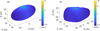 |
Fig. 14 Maximum radii of stable (no-slide) particles, when the van der Waals force applied on all particles is F = 1 nN due to surface roughness (Persson & Biele 2022), and the coefficient of friction is µ = 1. |
4.2 Interaction and potential balance between regolith production and loss
If we consider a bare rock surface of 2016 HO3, thermal fatigue should also be able to generate regolith, though the efficiency will be different from single particle layer situations in Sect. 3.2. Another simplification is that initial cracks of 30 µm are assumed in all surface particles (Delbo et al. 2014). Initial cracks are required to trigger the growth in the current model. Therefore, the generation of initial cracks and their length also control the production rate of regolith. In terms of the generation of cracks on a bare surface, both micro-impacts and thermal fatigue play constructive roles. High-velocity-impact-induced crack growth has been measured in OC and CC meteorites (Michikami et al. 2019, 2023). Layer(s) of regolith will increase porosity, decrease thermal conductivity, and therefore decrease skin depth. As a result, if there is a relatively thick layer of regolith, then the bedrock is protected from thermal fatigue. On the other hand, if there is no regolith, the bedrock is exposed to diurnal temperature excursion and cracks will grow due to both transient processes. Therefore, no matter the relative efficiency between micro-impacts and thermal fatigue, it is highly improbable that 2016 HO3 has a strong bare surface without cracks. Even if there is no regolith, it is still easier to knock off some particles from a surface with cracks than conduct on a huge bare rock.
Taking one step further, if we want to estimate the time required to reach a balance between micro-impacts and thermal fatigue and the equilibrated regolith distribution, the model at least needs to include porosity dependence of conductivity. Meanwhile, other second-order mechanisms, including electrostatic lofting (Hsu et al. 2022), solar radiation pressure, and self-gravity (Scheeres et al. 2010), might be important to determine where the equilibrium will end up. The present study does not include these second-order mechanisms or porosity and temperature dependence of physical properties evolving with diurnal thermal waves. Adding some of them would be an interesting direction for future study.
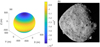 |
Fig. 15 Estimation of the surface dynamic environment of Bennu. (a) Summation of gravitational and centrifugal acceleration on a simplified shape model of asteroid Bennu, with a bulk density of 1.19 kg/m3 (Scheeres et al. 2019). (b) Real surface image of asteroid Bennu showing more particles and boulders at the poles as compared with the equator region, which is consistent with the simulation results indicated in (a). Image credit to NASA/Goddard/University of Arizona, by the OSIRIS-REx spacecraft. |
4.3 Comparison with other asteroids
The escape velocities of Itokawa, Ryugu, and Bennu are 0.2 m/s (Fujiwara et al. 2006), 0.37 m/s (Okawa et al. 2022), and 0.2 m/s (Perry et al. 2022; Scheeres et al. 2019), respectively. Compared with Fig. 11, the velocity of a significant portion of ejecta exceeds the escape velocities of all three asteroids in all four micro-impact scenarios. Figure 15a shows the net gravitational and centrifugal acceleration on the surface of Bennu as an example of comparison. There is no fission failure region on Bennu, but Bennu will still lose almost all ejecta after micro-impacts. Therefore, the direct result of micro-impacts should be similar between 2016 HO3 and other larger and slower-spin asteroids. The following effects and processes in 2016 HO3, such as disturbance by the impact shock and migration on the surface, might deviate from those visited asteroids because of 2016 HO3’s relatively low gravitational acceleration compared to centrifugal acceleration. In addition, the close observation and sampling of 2016 HO3 will be a potential opportunity to better understand the mechanism of cohesion of regolith on the asteroid’s surface, and thus resolve the discrepancy of cohesive strength mentioned above (Walsh et al. 2019; Lauretta et al. 2022).
5 Conclusions
In this paper a 3D shape model was established for 2016 HO3 based on its available light curves, with simulated impact craters embedded on its surface. To investigate the existence of possible regolith, the influence of cleanliness, coefficient of friction, and shape of the asteroid on the particle size distribution was analyzed with the surface dynamic environment model. The surface cleanliness was the most important to host regolith owing to the van der Waals cohesive force, but local topography was also important for the regolith to rest, for instance, on the walls of craters that face toward the rotation axis. The results of regolith change rates from the micro-impact and thermal fatigue model suggest that it is highly possible that regolith exists on the surface of 2016 HO3. Even if we consider other disturbances that significantly weaken the van der Waals force and remove all the regolith, the existence of cracks on the surface is highly possible.
This work represents one of the endeavors to study the surface dynamics of small fast-rotating asteroids. The developed methods and derived results will be useful in helping to design exploration and sampling strategies for 2016 HO3 by the Tianwen-2 mission, and for other similar asteroids in future missions.
Acknowledgements
This work was supported by grants from the Research Grants Council of Hong Kong (RIF Project No.: R5043-19; Project No.: 15219821; Project No.: 15210520). We appreciate Dr. David Čapek and Dr. David Vokrouhlický for their help and sharing of their code for the thermal stress model. The authors would like to acknowledge the constructive review by the anonymous reviewer.
References
- Ballouz, R.-I., Ernst, C., Barnouin, O. S., et al. 2024, Nature Astronomy, in press [Google Scholar]
- Barnouin, O. S., Daly, M. G., Palmer, E. E., et al. 2019, Nat. Geosci., 12, 247 [Google Scholar]
- Bernardoni, E., Horányi, M., & Szalay, J. 2021, Planet. Sci. Jo., 2, 67 [NASA ADS] [CrossRef] [Google Scholar]
- Bottke, W. F., Vokrouhlický, D., Ballouz, R.-L., et al. 2020, AJ, 160, 14 [NASA ADS] [CrossRef] [Google Scholar]
- Capek, D., & Vokrouhlický, D. 2010, A&A, 519, A75 [NASA ADS] [CrossRef] [EDP Sciences] [Google Scholar]
- Castellanos, A. 2005, Adv. Phys., 54, 263 [NASA ADS] [CrossRef] [Google Scholar]
- Castro-Cisneros, J. D., Malhotra, R., & Rosengren, A. J. 2023, Commun. Earth Environ., 4, 1 [NASA ADS] [CrossRef] [Google Scholar]
- Daly, R. T., Ernst, C. M., Barnouin, O. S., et al. 2023, Nature, 616, 443 [CrossRef] [Google Scholar]
- de la Fuente Marcos, C., & de la Fuente Marcos, R. 2016, MNRAS, 462, 3441 [CrossRef] [Google Scholar]
- Delbo, M., Libourel, G., Wilkerson, J., et al. 2014, Nature, 508, 233 [Google Scholar]
- DellaGiustina, D. N., Emery, J. P., Golish, D. R., et al. 2019, Nat. Astron., 3, 341 [Google Scholar]
- Fujiwara, A., Kawaguchi, J., Yeomans, D., et al. 2006, Science, 312, 1330 [NASA ADS] [CrossRef] [Google Scholar]
- Glinka, G., & Shen, G. 1991, Eng. Fract. Mech., 40, 1135 [CrossRef] [Google Scholar]
- Grün, E., Zook, H. A., Fechtig, H., & Giese, R. H. 1985, Icarus, 62, 244 [NASA ADS] [CrossRef] [Google Scholar]
- Harris, A. W. 1996, in Lunar and Planetary Science, 27, 493 [NASA ADS] [Google Scholar]
- Henke, S., Gail, H.-P., Trieloff, M., Schwarz, W. H., & Kleine, T. 2012, A&A, 537, A45 [NASA ADS] [CrossRef] [EDP Sciences] [Google Scholar]
- Hergenrother, C. W., & Whiteley, R. J. 2011, Icarus, 214, 194 [NASA ADS] [CrossRef] [Google Scholar]
- Horányi, M., Szalay, J. R., Kempf, S., et al. 2015, Nature, 522, 324 [CrossRef] [Google Scholar]
- Housen, K. R., & Holsapple, K. A. 2011, Icarus, 211, 856 [NASA ADS] [CrossRef] [Google Scholar]
- Housen, K. R., Wilkening, L. L., Chapman, C. R., & Greenberg, R. 1979, Icarus, 39, 317 [NASA ADS] [CrossRef] [Google Scholar]
- Hsu, H. W., Wang, X., Carroll, A., Hood, N., & Horányi, M. 2022, Nat. Astron., 6 [Google Scholar]
- Hughes, D. S., & Jones, H. J. 1950, Bull. Geol. Soc. Am., 61, 843 [NASA ADS] [CrossRef] [Google Scholar]
- Jiao, Y., Cheng, B., Huang, Y., et al. 2024, Nat. Astron., 8, 819 [NASA ADS] [CrossRef] [Google Scholar]
- Kaasalainen, M., Torppa, J., & Muinonen, K. 2001, Icarus, 153, 37 [NASA ADS] [CrossRef] [Google Scholar]
- Lauretta, D. S., Adam, C. D., Allen, A. J., et al. 2022, Science, 377, 285 [NASA ADS] [CrossRef] [Google Scholar]
- Levison, H. F., Marchi, S., Noll, K. S., et al. 2024, Nature, 629, 1015 [NASA ADS] [CrossRef] [Google Scholar]
- Li, X., & Scheeres, D. J. 2021, Icarus, 357 [Google Scholar]
- Li, X., Scheeres, D. J., Qiao, D., & Liu, Z. 2023, Astrodynamics, 7, 31 [NASA ADS] [CrossRef] [Google Scholar]
- Li, C., Liu, J., X., R., et al. 2024, J. Deep Space Explor., 11, 304 [Google Scholar]
- Loubser, P. J., & Bryden, J. G. 1972, Mag. Concrete Res., 24, 97 [Google Scholar]
- Matsumoto, M., Matsuno, J., Tsuchiyama, A., et al. 2024, Sci. Adv., 10, 1 [CrossRef] [Google Scholar]
- Mel’nikova, N. V., Rzhevskogo, V. V., & Protod’yakonova, M. M. 1975, Sprav-ochnik (Kadastr) Fisicheskikh Svoystv Gornykh Porod (Handbook [Registry] of Physical Properties of Rocks) (Nedra, Moscow), 279 [Google Scholar]
- Michikami, T., Hagermann, A., Tsuchiyama, A., et al. 2019, Planet. Space Sci., 177, 104690 [NASA ADS] [CrossRef] [Google Scholar]
- Michikami, T., Tsuchiyama, A., Hagermann, A., et al. 2023, Icarus, 392, 115371 [NASA ADS] [CrossRef] [Google Scholar]
- Misener, A. D., Thompson, L. G. D., & Uffen, R. J. 1951, Eos, Trans. Am. Geophys. Union, 32, 729 [CrossRef] [Google Scholar]
- Miyamoto, H., Yano, H., Scheeres, D. J., et al. 2007, Science, 316, 1011 [CrossRef] [Google Scholar]
- Molaro, J. L., Walsh, K. J., Jawin, E. R., et al. 2020, Nat. Commun., 11, 1 [CrossRef] [Google Scholar]
- Morota, T., Sugita, S., Cho, Y., et al. 2020, Science, 368, 654 [NASA ADS] [CrossRef] [Google Scholar]
- Müller, T. G., Durech, J., Ishiguro, M., et al. 2017, A&A, 599, A103 [NASA ADS] [CrossRef] [EDP Sciences] [Google Scholar]
- Naidu, S. P., Benner, L. A., Brozovic, M., et al. 2020, Icarus, 348, 113777 [CrossRef] [Google Scholar]
- Nakamura, T., Noguchi, T., Tanaka, M., et al. 2011, Science, 333, 1113 [NASA ADS] [CrossRef] [Google Scholar]
- Nelson, J. D. 1967, Environmental Effects on Engineering Properties of Simulated Lunar Soils (Illinois Institute of Technology) [Google Scholar]
- Nelson, J. D., & Vey, E. 1968, J. Geophys. Res., 73, 3747 [NASA ADS] [CrossRef] [Google Scholar]
- Nesvorný, D., Jenniskens, P., Levison, H. F., et al. 2010, ApJ, 713, 816 [CrossRef] [Google Scholar]
- Noguchi, R., Hirata, N., Hirata, N., et al. 2021, Icarus, 354, 114016 [NASA ADS] [CrossRef] [Google Scholar]
- Okawa, H., Arakawa, M., Yasui, M., et al. 2022, Icarus, 387, 115212 [NASA ADS] [CrossRef] [Google Scholar]
- Park, R. S., Konopliv, A. S., Bills, B. G., et al. 2016, Nature, 537, 515 [NASA ADS] [CrossRef] [Google Scholar]
- Perko, H. A., Nelson, J. D., & Sadeh, W. Z. 2001, J. Geotech. Geoenviron. Eng., 127, 371 [CrossRef] [Google Scholar]
- Perry, M. E., Barnouin, O. S., Daly, R. T., et al. 2022, Nat. Geosci., 15, 447 [NASA ADS] [CrossRef] [Google Scholar]
- Persson, B. N., & Biele, J. 2022, Tribol. Lett., 70, 1 [CrossRef] [Google Scholar]
- Pravec, P., & Harris, A. W. 2000, Icarus, 148, 12 [NASA ADS] [CrossRef] [Google Scholar]
- Reddy, V., Sanchez, J. A., Bottke, W. F., et al. 2016, AJ, 152, 162 [NASA ADS] [CrossRef] [Google Scholar]
- Reddy, V., Kuhn, O., Thirouin, A., et al. 2017, in AAS/Division for Planetary Sciences Meeting Abstracts #49, 204 [Google Scholar]
- Robinson, M. S., Thomas, P. C., Veverka, J., Murchie, S. L., & Wilcox, B. B. 2002, Invited Review The geology of 433 Eros, 37, 1651 [Google Scholar]
- Rognon, P. G., Roux, J. N., Naaïm, M., & Chevoir, F. 2008, J. Fluid Mech., 596, 21 [NASA ADS] [CrossRef] [Google Scholar]
- Russell, C. T., Raymond, C. A., Coradini, A., et al. 2012, Science, 336, 684 [NASA ADS] [CrossRef] [Google Scholar]
- Sánchez, P., & Scheeres, D. J. 2020, Icarus, 338, 113443 [Google Scholar]
- Sanchez, P., Azéma, E., Hoover, C., et al. 2023, AAS/Division for Planetary Sciences Meeting Abstracts, 55, 501 [Google Scholar]
- Scheeres, D. J., Hartzell, C. M., Sánchez, P., & Swift, M. 2010, Icarus, 210, 968 [NASA ADS] [CrossRef] [Google Scholar]
- Scheeres, D. J., McMahon, J. W., French, A. S., et al. 2019, Nat. Astron., 3, 352 [NASA ADS] [CrossRef] [Google Scholar]
- Sharkey, B. N., Reddy, V., Malhotra, R., et al. 2021, Commun. Earth Environ., 2 [CrossRef] [Google Scholar]
- Sierks, H., Barbieri, C., Lamy, P. L., et al. 2015, Science, 347, 1 [CrossRef] [Google Scholar]
- Spencer, J. R., Lebofsky, L. A., & Sykes, M. V. 1989, Icarus, 78, 337 [Google Scholar]
- Tsuchiyama, A., Uesugi, M., Matsushima, T., et al. 2011, Science, 333, 1125 [NASA ADS] [CrossRef] [Google Scholar]
- Veverka, J., Farquhar, B., Robinson, M., et al. 2001, Nature, 413, 390 [NASA ADS] [CrossRef] [Google Scholar]
- Walsh, K. J., Jawin, E. R., Ballouz, R. L., et al. 2019, Nat. Geosci., 12, 242 [NASA ADS] [CrossRef] [Google Scholar]
- Walsh, K. J., Ballouz, R. L., Jawin, E. R., et al. 2022, Sci. Adv., 8, 1 [NASA ADS] [Google Scholar]
- Waples, D. W., & Waples, J. S. 2004, Nat. Resour. Res., 13, 123 [CrossRef] [Google Scholar]
- Warner, B.D., Harris, A.W., & Pravec, P. 2021, Asteroid Lightcurve Database (LCDB) Bundle V4.0, https://doi.org/10.26033/j3xc-3359 [Google Scholar]
- Watanabe, S., Hirabayashi, M., Hirata, N., et al. 2019, Science, 364, 268 [NASA ADS] [Google Scholar]
- Werner, R. A., & Scheeres, D. J. 1996, Celest. Mech. Dyn. Astron., 65, 313 [NASA ADS] [Google Scholar]
- Whiteley, R. J., Tholen, D. J., & Hergenrother, C. W. 2002, Icarus, 157, 139 [NASA ADS] [CrossRef] [Google Scholar]
- Yamamoto, S., Kadono, T., Sugita, S., & Matsui, T. 2005, Icarus, 178, 264 [NASA ADS] [CrossRef] [Google Scholar]
- Yano, H., Kubota, T., Miyamoto, H., et al. 2006, Science, 312, 1350 [NASA ADS] [CrossRef] [Google Scholar]
- Yu, Y., & Baoyin, H. 2015, Astrophys. Space Sci., 355, 43 [NASA ADS] [CrossRef] [Google Scholar]
- Zhang, Y., Yan, X., Li, J., & Zeng, X. 2021, Mech. Eng., 43, 674 [Google Scholar]
All Tables
Basic information of some asteroids and their moonlets as targets of space missions.
All Figures
|
Fig. 1 Shape model of 2016 HO3 derived from light-curve inversion. Top four rows: examples of light curves (red dots) and the corresponding fits (solid lines) for estimating the shape of 2016 HO3. Bottom row: estimated 3D shape model of 2016 HO3. |
| In the text | |
|
Fig. 2 Shape models, (a) Model A. (b) Top view of Model B. (c) Bottom view of Model B. |
| In the text | |
|
Fig. 3 Magnitudes of gravitational accelerations. |
| In the text | |
|
Fig. 4 Escape velocities |
| In the text | |
|
Fig. 5 Net gravitational and centrifugal acceleration normal to the surface faces, with measured rotation period of 0.467 h. Outward is defined as the positive direction. For both Model A and B, outward accelerations are shown in the warm color scale (yellow to red) and inward accelerations are shown in the cold color scale (green to blue). |
| In the text | |
|
Fig. 6 Different dynamic regions resulting from the effects of gravity, centrifugal acceleration, and friction (coefficient µ = 1). The fission failure regions (where anet0 > 0) are labeled in blue, the landslide regions are in yellow, and the stable regions are in green.) |
| In the text | |
|
Fig. 7 Net outward normal acceleration from gravity, centrifugal force, and van der Waals forces. Under the choice of surface parameters, S = 0.1 and r = 1 mm, the van der Waals force dominates the surface dynamical environment. |
| In the text | |
|
Fig. 8 Maximum particle radii to avoid fission failure when S = 0.1. Red shows both landslide and stable regions that are not applied to this non-fission maximum radius calculation. |
| In the text | |
|
Fig. 9 Maximum radii of stable particles that will not slide under the coefficient of friction of µ = 1 and the cleanliness S = 0.1. |
| In the text | |
|
Fig. 10 Cumulative area distribution for the maximum grain diameters to avoid both landslide and fission failures. Panel a shows the results for shape Model A, and panel b shows the results for shape Model B. For each model, distributions for different parameter combinations, cleanliness S ∊ {1, 0.1, 0.01), and coefficient of friction µ ∊ {1, 0.5) are calculated. |
| In the text | |
|
Fig. 11 Mass of ejecta with velocities > υ for four individual micro-impact events, and the impact velocity is always 15 km/s. The two red lines show impacts on perlite–sand mixture (PS) with high porosity (ϕ = 0.6), and the black lines show impacts on rock. Spherical impactors with diameters of 100 µm and 200 µm are shown as solid and dashed lines, respectively. |
| In the text | |
|
Fig. 12 Time required to break rocks on 2016 HO3. Blue: carbonaceous chondrite; orange: ordinary chondrite; and purple: norite. The symbols for ordinary chondrite have been manually shifted slightly upward to show the uncertainty bars more clearly. |
| In the text | |
|
Fig. 13 Comparison of the regolith loss rate from micro-impacts (brown shaded area) and the regolith production rate from thermal fatigue. Surface materials are set to be (a) carbonaceous chondrite, (b) ordinary chondrite, and (c) norite. |
| In the text | |
|
Fig. 14 Maximum radii of stable (no-slide) particles, when the van der Waals force applied on all particles is F = 1 nN due to surface roughness (Persson & Biele 2022), and the coefficient of friction is µ = 1. |
| In the text | |
|
Fig. 15 Estimation of the surface dynamic environment of Bennu. (a) Summation of gravitational and centrifugal acceleration on a simplified shape model of asteroid Bennu, with a bulk density of 1.19 kg/m3 (Scheeres et al. 2019). (b) Real surface image of asteroid Bennu showing more particles and boulders at the poles as compared with the equator region, which is consistent with the simulation results indicated in (a). Image credit to NASA/Goddard/University of Arizona, by the OSIRIS-REx spacecraft. |
| In the text | |
Current usage metrics show cumulative count of Article Views (full-text article views including HTML views, PDF and ePub downloads, according to the available data) and Abstracts Views on Vision4Press platform.
Data correspond to usage on the plateform after 2015. The current usage metrics is available 48-96 hours after online publication and is updated daily on week days.
Initial download of the metrics may take a while.