| Issue |
A&A
Volume 692, December 2024
|
|
|---|---|---|
| Article Number | A207 | |
| Number of page(s) | 19 | |
| Section | Interstellar and circumstellar matter | |
| DOI | https://doi.org/10.1051/0004-6361/202451000 | |
| Published online | 13 December 2024 | |
Pulsar-wind nebulae meeting the circumstellar media of their progenitors
1
Institute of Space Sciences (ICE, CSIC),
Campus UAB, Carrer de Can Magrans s/n,
08193
Barcelona,
Spain
2
Laboratoire Univers et Théories, Observatoire de Paris, Université PSL, Université de Paris, CNRS,
92190
Meudon,
France
3
Institut d’Estudis Espacials de Catalunya (IEEC),
08034
Barcelona,
Spain
4
Institució Catalana de Recerca i Estudis Avançats (ICREA),
08010
Barcelona,
Spain
★ Corresponding author; This email address is being protected from spambots. You need JavaScript enabled to view it.
Received:
5
June
2024
Accepted:
24
September
2024
Abstract
Context. A significative fraction of high-mass stars sail away through the interstellar medium of the galaxies. Once they evolved and died via a core-collapse supernova, a magnetised, rotating neutron star (a pulsar) is usually left over. The immediate surroundings of the pulsar is the pulsar wind, which forms a nebula whose morphology is shaped by the supernova ejecta and channelled into the circumstellar medium of the progenitor star in the pre-supernova time.
Aims. Irregular pulsar-wind nebulae display a large variety of radio appearances, screened by their interacting supernova blast wave, or harbour asymmetric up–down emission.
Methods. Here, we present a series of 2.5-dimensional (2 dimensions for the scalar quantities plus a toroidal component for the vectors) non-relativistic magneto-hydrodynamical simulations exploring the evolution of the pulsar-wind nebulae generated by a red supergiant and a Wolf-Rayet massive supernova progenitor, moving with Mach number M = 1 and M = 2 into the warm phase of the Galactic plane. In such a simplified approach, the progenitor’s direction of motion, the local ambient medium magnetic field, and the progenitor and pulsar axis of rotation, are all aligned; this restricted our study to peculiar pulsar-wind nebula of high-equatorial-energy flux.
Results. We find that the reverberation of the termination shock of the pulsar-wind nebulae, when sufficiently embedded into its dead stellar surroundings and interacting with the supernova ejecta, is asymmetric and differs greatly as a function of the past circumstellar evolution of its progenitor, which reflects into their projected radio synchrotron emission. This mechanism is particularly at work in the context of remnants involving slowly moving or very massive stars.
Conclusions. We find that the mixing of material in plerionic core-collapse supernova remnants is strongly affected by the asymmetric reverberation in their pulsar-wind nebulae.
Key words: radiation mechanisms: non-thermal / stars: massive / stars: neutron / pulsars: general / stars: Wolf-Rayet / ISM: supernova remnants
© The Authors 2024
 Open Access article, published by EDP Sciences, under the terms of the Creative Commons Attribution License (https://creativecommons.org/licenses/by/4.0), which permits unrestricted use, distribution, and reproduction in any medium, provided the original work is properly cited.
This article is published in open access under the Subscribe to Open model. This email address is being protected from spambots. You need JavaScript enabled to view it. to support open access publication.
1 Introduction
Pulsars are the leftovers of dying massive stars, which gravitationally collapse after having consumed their nuclear fuel (Baade & Zwicky 1934). The conservation of angular momentum in the last seconds of massive star evolution provides neutron stars with their peculiar rotational and magnetic properties, potentially spinning up to millisecond frequencies and exhibiting a magnetic field strength reaching up to 1015 G (Manchester et al. 2005; Lorimer 2008). The formation of neutron stars is accompanied by the production of gravitational waves when the supernova is asymmetric (Taylor & Weisberg 1982; Kotake 2013) and closely related to the production of neutrinos (Kuroda et al. 2012; Kotake et al. 2012; Gabler et al. 2021; Shibagaki et al. 2024). The pulsar might receive a natal kick, potentially accelerating it to speeds of the order of 100–1000 km s−1 (Pavan et al. 2016; Verbunt et al. 2017; de Vries et al. 2021). Once born, the pulsar generates a relativistic wind made of leptons, which is blown into such plerionic supernova ejecta. The region filled with this material is called a pulsar-wind nebula (see e.g. Reynolds & Chevalier 1984).
Plerions are therefore supernova remnants that contain a pulsar wind, which is archetypical; (Hester 2008; Bühler & Blandford 2014; Bock et al. 1998; Popov et al. 2019; H.E.S.S. Collaboration 2019). Pulsar wind nebulae emit non-thermally at all frequencies, complicating the distinction with the supernova remnant in the system (Weiler & Shaver 1978; Caswell 1979; Weiler & Panagia 1980). This emission relates to the continuous injection of relativistic particles in the magnetised pulsar wind blown by the rotating neutron star (pulsar), and it is affected by their dynamics; we invite the reader to consult, e.g., Atoyan & Aharonian (1996); Gelfand et al. (2009); Bucciantini et al. (2011); Martin et al. (2012); Torres et al. (2014); Martin & Torres (2022).
Pulsar winds act as an additional component influencing the generic process of a supernova blast wave propagating into the interstellar medium (ISM) of galaxies (Chevalier 1982), which is itself impacted by the circumstellar medium shaped by the massive progenitor stars of type II, core-collapse supernovae (Chevalier & Liang 1989; Orlando et al. 2019, 2021, 2020, 2022). The pulsar wind first propagates into the freely expanding explosion material before interacting with the termination shock of the supernova ejecta, producing a pulsar bubble developing strong Rayleigh-Taylor instabilities at the pulsar wind or at the supernova ejecta contact discontinuity (Reynolds & Chevalier 1984; Blondin et al. 2001; van der Swaluw 2003). Specifically, the interaction of the supernova blast wave with the circumstellar medium is responsible for a variety of observed features, for example in the light curves of the growing remnants (Soker & Kaplan 2021; Soker 2023a,b; Shishkin & Soker 2023). The shocked pulsar-wind material changes at different stages of the further evolution by adopting the morphology of a bow shock under the influence of the neutron star intrinsic motion (Kulkarni & Hester 1988), by developing kinked, jetlike features as the neutron star spins fast (Weisskopf et al. 2013), or by having its termination shock reverberated towards the pulsar (Bandiera et al. 2021, 2023a,b)
The modelling of pulsar-wind nebula has been mostly driven by the study of the Crab nebula and a few other iconic historical plerions such as Geminga and Vela, driving theoretical advances (Kennel & Coroniti 1984; Coroniti 1990; Begelman & Li 1992; Begelman 1998), axisymmetric simulations (Del Zanna et al. 2006; Camus et al. 2009; Komissarov & Lyutikov 2011; Olmi et al. 2014), and full 3D models (Porth et al. 2013, 2014; Olmi et al. 2016). The studies of Komissarov & Lyubarsky (2003, 2004); Del Zanna et al. (2004) and Komissarov (2006) demonstrate that polar wind nebulae produce a diamond-like morphology, made of an equatorial region pushed by the magneto- rotational properties of the pulsar magnetosphere plus a polar double jet growing perpendicularly to the disc. At early times, the pulsar wind leaves the surface of the magnetosphere of the spinning neutron star and interacts with its immediate environment (see the reviews of Gaensler & Slane 2006; Kargaltsev et al. 2017; Olmi & Bucciantini 2023 for details). This explains the multi-wavelength emission of plerions predominantly governed by non-thermal synchrotron and inverse Compton radiation (see Atoyan & Aharonian 1996; Reynolds et al. 2017) as well as radio (Driessen et al. 2018), X-rays, and (up to PeV) γ-rays (Borkowski et al. 2016; Aharonian et al. 2006; Abdalla et al. 2021; Lhaaso Collaboration 2021). Current and forthcoming ground-based, high-energy facilities such as LHAASO and CTA are particularly intended for the study of those emissions (for recent discussions see, e.g. Mestre et al. 2022; Acero et al. 2023, and references therein).
On a larger scale, more global simulations have been performed in order to address the question of pulsar-wind nebulae as an essential component of the internal functioning of older (>10 kyr) core-collapse supernova remnants. There, the pulsar wind interacts with the supernova ejecta and reverberates, during and after which the morphology, spectrum, and dynamics of pulsar-wind nebulae could undergo significant changes (see the recent studies by Bandiera et al. 2020, 2023a,b). The bulk motion of the kicked pulsar throughout the supernova ejecta and the distortion of pulsar-wind nebulae into bow shocks were modelled in the studies of van der Swaluw et al. (2003, 2004); Bucciantini et al. (2004); Temim et al. (2017); Kolb et al. (2017); Temim et al. (2022), in the frames of hydrodynamics, magnetohydrodynamics, and relativistic magnetohydrodynamics. Applications to specific objects are numerous, which can be seen, for instance, in the cases of the supernova remnant G292.0+1.8 (Temim et al. 2022), supernova remnant MSH 15–56 (Temim et al. 2017), and supernova remnant G327.1-1.1 (Temim et al. 2015). The pulsar will eventually leave the still-expanding supernova remnant and pass through the forward shock of the supernova blast wave to finally interact with the ISM (Bucciantini & Bandiera 2001; Bucciantini 2018; Toropina et al. 2019).
The modelling of supernova remnants of massive runaway stars is motivated by two facts. On the one side, up to half of high-mass stars are fast-moving objects sailing through the ISM; therefore, the inclusion of stellar motion in the models is an essential parameter to account for their understanding. On the other hand, the interaction mechanism at work when a supernova blastwave collides with the dense stellar-wind bow shocks those stars produce is more prone to inducing asymmetric structures than when the pre-supernova circumstellar medium is spherically symmetric (Velázquez et al. 2006; Chiotellis et al. 2013; Meyer et al. 2015).
So far, the effects of the stellar motion on the off-centring of the explosion into the stellar-wind bubble of a 60 M⊙ (Groh et al. 2014) was examined in the work of Meyer et al. (2020). How the coupling of the stellar bulk motion with the mass-loss history of a 35 M⊙ Wolf-Rayet supernova progenitor (Ekström et al. 2012) affects the non-thermal radio emission of core-collapse supernova remnants is studied in Meyer et al. (2021b); they demonstrated that bilateral and horseshoe-like remnant morphologies are natural consequences of the radio emission. The mixing of materials (stellar wind, ejecta) in such supernova remnants has been modelled in Meyer et al. (2023). In Meyer & Meliani (2022) and Meyer et al. (2024a), we simulated the additional incidence of a pulsar wind into the above-described core-collapse supernova remnants, showing that the pre-supernova distribution of circumstellar material governs the evolution of older pulsar-wind nebulae, in the contexts of a moving (Meyer & Meliani 2022) and a static (Meyer et al. 2024a) progenitor star. The present work expands on those simulation methodologies.
As well as the precedent works of our present study, it is characterised by two main assumptions. The first is the choice of an axisymmetric setup, where the direction of motion and the axis of rotation of the progenitor star, the direction of the local ISM magnetic field, and the pulsar axis of rotation are aligned; this is because of the intrinsic nature of the used coordinate system. This restricts us to the production of results applying to peculiar pulsar-wind nebulae, which are shaped by their higher equatorial energy flux. Hence, our models only apply to a specific part of the huge parameter space of the pulsar-wind-nebula problem. We decided to investigate it first since the use of axisymmetric simulations allowed us to reach high spatial resolutions across large regions of space over long time frames. Secondly, the plerionic supernova remnants are treated within the non-relativistic regime. By carrying out classical simulations and using significantly slower pulsar winds (recall that the wind can reach Lorentz factors as high as 106 e.g. Kennel & Coroniti 1984) we have access to a more stable simulation setup that is more suitable for exploring the parameter space in terms of stellar evolution history. However, reducing the pulsar-wind speed can alter several aspects of the pulsar-wind nebulae evolution, including compression rates, shock velocities and the development of associated instabilities. However, it is important to note that the momentum of the flow is the primary factor influencing the strength of the shock (Wilkin 1996). By using a lower wind speed, we aim to provide a preliminary estimate for the evolution of pulsar-wind nebulae.
We adopted a low magnetisation value of σ = 10−3, as described by Rees & Gunn (1974), Kennel & Coroniti (1984), Slane (2017), Begelman & Li (1992), and Torres et al. (2014). This choice reflects the assumption that a significant portion of the magnetic field energy is converted into kinetic energy within the pulsar-wind nebulae. Recent multi-dimensional simulations, however, have demonstrated that higher magnetisation values, such as σ = 0.01 in two-dimensional (e.g. Komissarov & Lyubarsky 2003, 2004; Del Zanna et al. 2004, 2006) and even σ > 1 in 3D (Porth et al. 2014; Barkov et al. 2019), are more effective in reproducing the features of pulsarwind nebula termination shocks. The magnetisation of the pulsar wind is a topic of ongoing debate, as it significantly influences the strength of the pulsar-wind nebula termination shock and, consequently, particle acceleration processes. Furthermore, the magnetisation in the equatorial wind zone may decrease due to the annihilation of magnetic stripes, leading to lower effective magnetisation values (Coroniti 2017). By opting for a low magnetisation value, similar to that used by Bucciantini et al. (2004), the pulsar-wind nebulae in our simulations tend to expand more in the equatorial plane, resulting in a stronger termination shock.
This study investigated the effects of the circumstellar medium of runaway rotating massive stars moving in the magnetised warm phase of the Galactic plane on the morphology and non-thermal emission properties of the pulsar-wind nebulae that they generate once they have died and exploded as corecollapse supernova remnants. A representative parameter space of the identity of supernova progenitors is scanned, using initial stellar masses of 20 M⊙ (the so-called red supergiant progenitor) and 35 M⊙ (the so-called Wolf-Rayet progenitors), together with space velocities of 20 and 40 km s−1. It extends the study of Meyer & Meliani (2022) to several other progenitor stars, both in terms of the zero-age main sequence, i.e., assuming different evolutionary paths, and bulk motion through the ISM. This results in a changing distribution of the circumstellar material at the moment of the supernova explosion, which releases a blast wave channeled into it and influencing the morphology of the pulsar-wind nebula accordingly.
The paper is organised as follows. Section 2 presents the utilised numerical methods. The results are detailed in Sect. 3 and discussed in Sect. 4. The conclusions of this study are drawn in Sect. 5.
2 Method
In this section, we review the numerical methods, initial conditions, and physical processes included in the magneto- hydrodynamical simulations, as well as the methodology used to derive the non-thermal radio-emission maps.
2.1 Numerical setup
2.1.1 Pre-supernova circumstellar medium
The wind-ISM interaction of the moving supernova progenitor is calculated throughout the entire massive star’s life, from its main-sequence age to the pre-supernova time. We used a cylindrical computational domain of [0; Rmax] × [zmin; zmax], where Rmax = 100 pc and zmax = |zmin| = 50 pc, which is mapped with a uniform mesh of 2000 × 2000 grid zones. Axisymmetry is imposed in the toroidal direction. The z-axis is chosen in the direction in which the runaway massive star moves. Inflow boundary conditions are imposed at z = zmax , while outflow boundary conditions are assigned to z = zmin and R = Rmax , respectively, since the evolution of the wind-ISM interaction is calculated in the frame of the moving star; that is, by imposing
 (1)
(1)
at z = zmax as well as everywhere in the domain. Here, v★ is the velocity of the moving star with respect to the ISM (Comerón & Kaper 1998). The ISM magnetic field is initially everywhere, and at z = zmax it is
 (2)
(2)
where BISM = 7 µG is the strength of the magnetic field. The ISM magnetic field vector direction is also aligned with the axis of symmetry of the computational domain. The ISM density is initially taken to match that of the warm phase of the Galactic plane nISM ≈ 0.79 cm−3 for a temperature of TISM ≈ 8000 K (see Meyer & Meliani 2022).
2.1.2 Supernova remnant and pulsar-wind nebula phase
At the supernova time, we remap the wind-ISM solution onto a computational domain of smaller size and higher spatial resolution (i.e. a 2.5-dimensional cylindrical coordinate system Rmax = zmax = |zmin| = 25 pc with a uniform mesh of 4000 × 8000 grid zones), into which we inject a supernova blast wave. We then inject a pulsar wind into the computational domain, at the location of the defunct runaway star. The spatial resolution of the wind-ISM grid is therefore 0.05 pc, while that of the pulsarwind nebulae grid is 0.00625 pc. The simulation methodology is that typically used for the modelling of middle-age supernova remnants. The entire circumstellar medium of the supernova progenitor is first calculated accounting for its stellar evolution history. In a second step, the stellar-wind bow shock is used to model the interaction between the supernova blast wave and its surrounding medium. Last, a pulsar wind is injected at the location of the ejecta. Hence, one obtains a consistent picture of the evolution of the pulsar-wind nebula. This is governed by the distribution of supernova ejecta, which are themselves rules by the circumstellar medium (Meyer & Meliani 2022; Meyer et al. 2024a).
2.1.3 Numerical methods
The simulations are carried out using the PLUTO code (Mignone et al. 2007, 2012)1. The adopted numerical scheme uses a finite- volume formulation with a Godunov-type solver made using a Harten-Lax-van Leer (HLL) Rieman solver (Harten et al. 1983) for flux computation; a parabolic reconstruction for spatial accuracy; a minmod limiter for flux limiting; a third-order Runge Kutta (RK3) for time-stepping; and the Courant–Friedrich–Levy condition, initially set to Ccfl = 0.1, for determining the time step. The use of the eight-wave algorithm (Powell 1997) ensures that ∇ ⋅ B = 0 throughout the calculation domain.
2.2 Governing equations
Plasma magneto-hydrodynamics obeys the standard equations for the conservation of the density,
 (3)
(3)
linear momentum vector,
 (4)
(4)
total energy,
 (5)
(5)
and magnetic field,
 (6)
(6)
where ρ is the mass density, v the velocity vector, m = ρv the momentum vector, Î the identity vector, B the magnetic field vector, pt = p + B2/8π the total pressure2, and
 (7)
(7)
the total energy with γ = 5/3 as the adiabatic index. The system is evolved under the assumption of an ideal equation of state and the governing equations are closed with
 (8)
(8)
where cs is the sound speed of the plasma.
The right side of the energy conservation equation is
 (9)
(9)
where Γ(T) and Λ(T) are the heating and cooling rates, respectively,
 (10)
(10)
is the gas temperature, nH is the hydrogen number density, kB is the Boltzmann constant, µ is the mean molecular weight, and nH = ρ/(µmH(1 + χHe,Z)) with χHe,z as the mass fraction of the species heavier than H. The heating and cooling laws for ionised gases were derived in Meyer et al. (2014) and are used in the calculation for the pre-supernova-remnant phase and the early supernova blast-wave stellar-wind interaction. These terms are ignored once the pulsar wind is launched and when the system is evolved adiabatically.
2.3 Magnetic stellar wind
A stellar-wind density profile is set on a sphere with a radius equal to 20 grid zones centred at the origin:
 (11)
(11)
where Ṁ(t) is the time-dependent mass-loss rate of the progenitor star, interpolated from the stellar evolutionary tracks of the GENEVA library (Ekström et al. 2012). The wind terminal velocity is calculated using the recipe of Eldridge et al. (2006). In Fig. 1, we report the time evolution of the stellar mass, wind velocity, and mass-loss rate used in this study. The supernova progenitors are selected with initial rotation at the equator, such that
 (12)
(12)
with Ω★(t = 0) being the rotational velocities and ΩK the Keplerian velocity at the equator, respectively. The toroidal component of the wind velocity therefore reads
 (13)
(13)
with θ being the azimuthal angle, such that
 (14)
(14)
(see Chevalier & Luo 1994; Rozyczka & Franco 1996). The magnetic field in the stellar wind is assumed to be a Parker spiral of the radial component
 (15)
(15)
and the toroidal component
 (16)
(16)
here, the surface magnetic-field strength is set to B★ = 500, 0.2, = 100G for the main-sequence, red-supergiant, and Wolf- Rayet phases, respectively (see Vlemmings et al. 2002, 2005; Fossati et al. 2015; Castro et al. 2015; Przybilla et al. 2016; Castro et al. 2017; Kervella et al. 2018). This is scaled to the strength of the solar magnetic field (Scherer et al. 2020; Herbst et al. 2020; Baalmann et al. 2020, 2021; Meyer et al. 2021a).
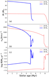 |
Fig. 1 Temporal evolution (in Myr) of supernova progenitors of zeroage main-sequence 20 M⊙ (dotted red line) and 35 M⊙ (solid blue line) considered in our study. The panels display the stellar mass M★ (panel a, in M⊙), wind velocity vw (panel b, in km s−1 ), and their mass-loss rate Ṁ (panel c; in M⊙ yr−1). |
Models in our study.
2.4 Supernova blast wave
The core-collapse supernova blast wave is imposed using the method developed by Truelove & McKee (1999) and Whalen et al. (2008); however, we refer the reader to our discussion Bandiera et al. (2021), particularly where we refer to the n parameter. It consists of imposing the following profiles for the mass density in the r ≤ rmax region of the computational domain:
 (17)
(17)
where
 (18)
(18)
and
 (19)
(19)
with Mej representing the ejecta mass and Eej the ejecta energy and n = 11 being an exponent typical for core-collapse supernova blast waves (Truelove & McKee 1999)3. Also,
 (20)
(20)
which is determined by the numerical iterative method described in Whalen et al. (2008).
The velocity field is set radially using the relation
 (21)
(21)
with
 (22)
(22)
and
 (23)
(23)
at the characteristic radii rcore and rmax , respectively, marking the transition between the plateau and the forward shock of the blast wave. The mass in the ejecta is chosen to be that of the progenitor at the moment of the explosion, minus the mass of the neutron star that is left behind; that is,
 (24)
(24)
with MNS = 1.4 M⊙ and with tZAMS and tSN the zero-age main- sequence and supernova times, respectively. The ejecta masses in the different models are reported in Table 1.
2.5 Pulsar wind
The pulsar-wind description is based on the method developed in Komissarov & Lyubarsky (2004). It is controlled by its timedependent total power,
 (25)
(25)
with
 (26)
(26)
where n is the braking index of the pulsar and Ė0 = 1038 erg s−1 is the initial pulsar-energy variation, and the initial spin-down is given by
 (27)
(27)
here, following Slane (2017), we set n = 3 for the pulsar’s magnetic dipole spin-down. The pulsar’s initial period is set to Po = 0.3 s and its time derivative is  . The model assumes a constant pulsar-wind velocity:
 (28)
(28)
with c being the speed of light. The mass-loss rate in the pulsar wind depends on its total power and velocity, which is given by
 (29)
(29)
therefore, its mass density is
 (30)
(30)
The pulsar-wind magnetisation is exclusively toroidal, with a magnetisation factor of σ = 10−3 (Slane 2017); thus,
 (31)
(31)
is the pulsar-wind magnetisation at the inner pulsar-wind radius rin of 20 grid zones (of the finer grid 4000 × 8000), within which the pulsar wind is continuously enforced. There is no evolution of the equations inside the inner boundary of radius rin , which is eight times smaller duing the pulsar wind phase, than during the wind-ISM phase. This remapping of the wind-ISM solution onto a finer grid at the pre-supernova time prior to the launching of the pulsar wind is necessary to avoid problems due to reverberation and the termination shock potentially hitting the inner boundary.
A passive scalar tracer Qpsr = 1 is injected into the pulsar wind with an initial value of Qpsr = 0 elsewhere. It obeys the advection equation,
 (32)
(32)
which allows the time-dependent tracking of the transport of leptonic material into the supernova ejecta and the defunct circumstellar medium.
2.6 Radiative transfer calculations
We generate emission maps from the magneto-hydrodynamical simulations. The three-dimensional structure of the gas density and magnetic field in the pulsar-wind nebula are reconstructed from the 2.5-dimensional models accounting for their axisymmetric nature (Meyer et al. 2021b). We present the maps in normalised units, with relative arbitrary scale, which is done by assuming the non-thermal electron population to be described by the power-law distribution,
 (33)
(33)
where K is a proportionality constant and s = 2α + 1 is an index that is a function of the spectral index α. The synchrotron emissivity is given by
 (34)
(34)
where B⊥ is the component of the magnetic field that is normal to the line of sight and v is the emission frequency. The emission maps are obtained by integrating the emissivity along the line of sight,
 (35)
(35)
according to a given aspect angle θobs where dl is the line-of-sight differential length element (Meyer & Meliani 2022).
3 Results
This section presents the structure of the plerionic supernova remnants in our models and describes the non-thermal appearance of the pulsar-wind nebulae by synchrotron emission.
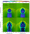 |
Fig. 2 Number density fields in our magneto-hydrodynamical simulation of the supernova remnant of the runaway 20 M⊙ star rotating with Ω★/ΩK = 0.1 and moving with velocity v★ = 20 km s−1. The evolution of the plerionic supernova remnant is shown at times 2.5 (a), 5.0 (b), 7.5 (c), and 12.5 kyr (d), respectively. The various black contours highlight the region with a 50% contribution of pulsar-wind material. The black arrows in the right parts of the figures are ISM magnetic field lines. |
3.1 Model with 20 M⊙ and v★=20 km s−1
Figure 2 shows the number-density fields in the model with a runaway red supergiant star with an initial mass of 20 M⊙ moving at a velocity of v★ = 20 km s−1. The panel plots the supernovaremnant structure at times 2.5 (a), 5.0 (b), 7.5 (c), and 12.5 kyr (d) after the onset of the supernova explosion, respectively. In the figure, the black contour marks the region of the remnant with a 50% contribution of pulsar-wind material in number density, while the black arrows in the right sections of the figures are ISM magnetic field lines.
At 2.5 kyr, the large-scale circumstellar medium occupies most of the computational domain, which is composed of the main-sequence stellar-wind bow shock in which the red supergiant wind has been blown. The main-sequence stellar-wind bow shock is a structure within which the region of unshocked wind material that is shaped as a low-density region that extends behind the dense arc of swept-up ISM gas accumulated during the life of the moving star. The red supergiant wind is a shell of slow, dense material that collided with the former bow shock and penetrated into it within a radius of ≈10 pc around the centre of the explosion.
Furthermore, the supernova blast wave, launched at the moment of the explosion, has in turn interacted with the circumstellar distribution of red-supergiant wind. This induces large Rayleigh-Taylor instabilities at the wind or at the ejecta contact discontinuity in which the pulsar-wind nebula develops, sweeping up the supernova ejecta (Fig. A.1a).
At 5.0 kyr, the supernova blast wave is now strongly interacting with the red-supergiant wind, creating a dense arc of swept- up material made of both stellar wind and ambient medium. The blast wave travels back towards the centre of the explosion, creating an additional ovoidal layer filled by a hot mixture of evolved stellar wind, ejecta and pulsar-wind materials extending up to about 4–7 pc from the origin, slightly losing sphericity as it pours out into the low-density tail of the bow shock (at z = −7 pc). The shape of the pulsar-wind nebula deviates from the diamondlike solution of Komissarov & Lyubarsky (2004); this is a direct result of its interaction with the ejecta, itself impacted by the circumstellar medium of the runaway progenitor (Fig. A.1b).
At 7.5 kyr and later, the plerionic supernova remnant has further evolved, in the sense that the spinning pulsar induces a double polar-jet-like feature, either interacting with the bow shock (z > 0 region of the figure) or expanding more freely into the low-density trail of material (z < 0 region of the figure). While the forward shock of the blast wave expands outwards, the power of the rotating neutron star sustains the reverberating termination shock of the pulsar-wind nebula, preventing it from recovering its diamond-like morphology. Consequently, the pulsar-wind nebula adopts a spinning-top shape that is conic in the upper part and jet-like in the lower region (Figs. A.1c, d).
3.2 Model with 20 M⊙ and v★ = 40 km s−1
Figure A.1 shows the number-density fields in the simulation model with a runaway red-supergiant star with an initial mass of 20 M⊙ moving at a velocity of v★ = 40 km s−1 ; this was already described in great detail in the preceding paper of this series (see Meyer & Meliani 2022). The circumstellar medium generated by the runaway massive star is different from that in the model with a velocity of v★ = 20 km s−1. Even if the stellar evolutionary stages it undergoes are similar, the morphology of the stellar- wind bow shock is different as a result of the bulk motion, which produces a smaller stand-off distance (Baranov et al. 1975) and a more compact bow shock (Wilkin 1996). The main-sequence bow shock is closer than in the model with v★ = 20 km s−1 and the cavity of lower-density material. The red-supergiant material is contained in a more reduced region, since the denser walls of the bow shock prevent it from penetrating deeply into the region of main-sequence material (Fig. A.1a).
The moving progenitor in the model with an initial mass of 20 M⊙ and a velocity of v★ = 40 km s−1 is the typical scenario leading to the production of a Cygnus Loop supernova remnant (Meyer et al. 2015), with an asymmetric propagation of the shockwave that is channelled by the azimuthal-dependent distribution of circumstellar material. Along the direction of motion of the progenitor, it interacts with the bow shock and further expands into the ISM, while in the opposite direction the blast wave propagates through the bow-shock tail (Figs. A.1a, b). The pulsar-wind nebula that grows inside this similarly to the Cygnus Loop prevents the blast-wave reverberation, while the morphology of the pulsar-wind nebula sees its shape distances from the diamond-like form of Komissarov & Lyubarsky (2004). In Meyer & Meliani (2022), it is shown that the spatial distribution of the region of shocked pulsar-wind material, located between the lepton and the ejecta contact discontinuity, is governed by a competition between the magneto-rotational intrinsic properties of the pulsar and the pre-supernova circumstellar medium. First, it becomes an ovoid region (Fig. A.1a); then, it exhibits important north-south asymmetries (Fig. A.1b) before ending up with a rather standard bipolar jet-plus-equatorial structure (Figs. A.1c, d).
3.3 Model with 35 M⊙ and v★ = 20 km s−1
Figure A.2 shows the number density fields in the simulation with a runaway Wolf-Rayet star with an initial mass of 35 M⊙ moving at a velocity of v★ = 20 km s−1 through the ISM. The presupernova circumstellar medium is made of a large ring of dense Wolf-Rayet material distributed at a radius of approximately 7–15 pc. The power of this last stellar wind has pushed the material away from the previous evolutionary phases of the massive star, and it mostly interacts with the bow shock rather than with the ISM (Brighenti & D’Ercole 1995b). The supernova blast wave is expanding into this ring and the pulsar wind material is expanding into the ejecta (Fig. A.2a), which has the diamondlike morphology described by Komissarov & Lyubarsky (2004). At 5.0 kyr, the supernova ejecta collides with the Wolf-Rayet ring and begins to travel back towards the centre of the explosion. A region of shocked ejecta material formed while the blast wave was still expanding downwards towards the tail of the bow shock.
The contact discontinuity of the pulsar-wind nebula interacts with the reverberating supernova blast wave and begins to lose the structure described in the study by Komissarov & Lyubarsky (2004). At 7.5 kyr, the pulsar wind is strongly interacting with the supernova ejecta and moving back to the region of the explosion in the z > 0 region of the supernova remnant. A series of unstable Rayleigh-Taylor layers form as a mechanism of double reverberation begins; the termination shock of the pulsar wind in turn moves back towards the centre of the explosion, while the termination shock of the supernova blast wave experiences a similar mechanism. At 12.5 kyr, the two termination shocks have met, giving birth to an overall region of mixed shocked ejecta and shocked pulsar wind engulfing the unshocked, still streaming pulsar-wind material and surrounded by the bow shock of the defunct stellar wind. As a consequence of the asymmetric distribution of circumstellar material, the reverberations are more important in the z > 0 region of the supernova remnant, producing an oblong pulsar-wind nebula. On the top of the shock, a jet-like feature develops and propagates until the outer border of the supernova remnant and to the ISM. The low-density region, regardless of the material (wind, ejecta, pulsar wind) it is composed of, is much larger in the context of a moving Wolf-Rayet supernova progenitor than that of a red supergiant star, and the properties of the mixed material change accordingly, as does as the size of the pulsar-wind nebula.
3.4 Model with 35 M⊙ and v★ = 40 km s−1
Figure A.3 shows the number density fields in the simulation model with a runaway Wolf-Rayet star with an initial mass of 35 M⊙ moving at a velocity of v★ = 40 km s−1 through the ISM. As in the models with initial masses of 20 M⊙ , the stellar-wind bow shock of the progenitor star is less open when it moves faster. Since the last stellar wind of the Wolf-Rayet phase is blown at a terminal speed exceeding that of the progenitor bulk motion, the ring of material penetrates directly into the unperturbed ISM (see description of this mechanism in Brighenti & D’Ercole 1995a). It is the site of huge Rayleigh–Taylor instabilities that deform the circumstellar ring. The expanding supernova blast wave hits the bow shock and fills the large eddies it developed and the typical diamond-like solution for the pulsar wind nebula forms in it (see Fig. A.3a). At this time, the pulsar-wind nebula is protected from information of the past evolution of the progenitor star. At 5.0 kyr, the pulsar wind has interacted with the reverberating supernova ejecta in the direction of stellar motion, while both the blast wave and pulsar wind still propagate freely in the other direction.
At 7.5 kyr, the reverberation of the supernova blast wave collides with the pulsar wind, which in turn experiences the reverberation process, ending as a swept-up region of shocked ejecta and pulsar-wind material that is surrounded by the ring of Wolf-Rayet stellar wind. The morphology of the pulsar wind is strongly deviating from the diamond-like solution of Komissarov & Lyubarsky (2004). This trend keeps going at later times, and, 12.5 kyr after the supernova explosion, the pulsar wind has adopted a shape similar to that in the model with a star of initial mass 35 M⊙ moving with velocity v★ = 40 km s−1 through the ISM, composed of an oblong region in which the pulsar is off-centred and a bipolar jet intercepts the dense former stellar-wind bow shock hit by the supernova blast wave (Fig. A.3d).
3.5 Radio synchrotron maps
Figure 3 plots synchrotron emission maps of the plerionic supernova remnant models in this study, calculated assuming an aspect angle of θobs = 45° between the observer’s line of sight and the plane of the sky. The figure displays the images as a function of time and of the initial conditions of the models, plotted in normalised units. Each column corresponds to a different time after the explosion, specifically 5 (left column), 7.5 (middle column), and 15.5 kyr (right column), respectively. Each row corresponds to a different supernova progenitor, namely an initial mass of 20 M⊙ moving at a velocity of v★ = 20 km s−1 (top line), an initial mass of 20 M⊙ moving at a velocity of v★ = 40 km s−1 (second row), an initial mass of 35 M⊙ moving at a velocity of v★ = 20 km s−1 (third row), and an initial mass of 35 M⊙ moving at a velocity of v★ = 40 km s−1 (bottom row), respectively. Figure B.1 is the same is Fig. 3, but it assumes an aspect angle of θobs =0°.
In turn, Fig. 4 plots horizontal cuts taken through the synchrotron radio-emission maps calculated in Fig. B.1, while Fig. C.1 plots vertical cuts taken through the synchrotron radioemission maps calculated with θobs = 0°. The disposition of the different panels corresponds to that of Figs. 3–B.1, comparing the emission for θobs = 0° (dashed blue line) and θobs = 45° (solid red line). The second row of panels (Figs. 3d–f) displays the maps already described in Meyer & Meliani (2022). Initially, the pulsar wind is absent from the z > 0 region that is along the direction of motion of its defunct progenitor star. When the polar jet of the pulsar wind begins interacting with the supernova ejecta and the shocked stellar wind, it becomes brighter than the walls of the cavity shaped prior to the explosion (Fig. 3e).
The north-south radio-flux difference increases as a function of time; the northern jet collides into the shocked supernova material, while the other one propagates in the cavity of low- density material (see Fig. 3f). The first row of panels corresponds to the model with a slower progenitor compared to that of the second line (Figs. 3a–c). Therein, the non-thermal flux from the circumstellar medium is much fainter than that of the pulsar wind, regardless of the time spent after the explosion and the onset of the pulsar wind. The north-south emission difference persists with a brighter northern part up to 7.5 kyr before being reversed at 12.5 kyr, when the southern part becomes brighter (Fig. 3c).
The model with a mass of 35 M⊙ and moving at a velocity of v★ = 20 km s−1 induces a very bright circumstellar medium that is much brighter than the pulsar-wind nebula, appearing as a larger scale synchrotron arc with a radius of 10 pc and whose flux surpasses that of the jet. At 7.5 kyr, the overall dense arc is even more luminous; however, the central pulsar-wind nebula induces an increasing surface brightness that competes with the region where the supernova blast wave interacts with the circumstellar medium (Fig. 3g). The expanding collimated wind of the spinning pulsar overwhelms the brightness of its surroundings made of mixed ejecta, stellar wind, and ISM at 12.5 kyr (Fig. 3j), as is the case in the other models (Figs. 3c,f). The last model with a 35 M⊙ progenitor moving with velocity v★ = 40 km s−1 has a circumstellar medium whose brightness is governed by a dense equatorial region where the ejecta meet the unstable circumstellar medium, inducing bright synchrotron rings (Fig. 3j). Throughout the entire modelled evolution of our plerion, the pulsar wind remains fainter than its surrounding supernova remnant, except in the very central region where the polar originates (see Fig. 3).
By comparing the emission maps at similar times, one notices that the region of the blast wave interacting with the circumstellar medium compresses the ISM magnetic field better in the case of a 35 M⊙ progenitor, screening the pulsar-wind nebula (see images at 5.0 kyr in Figs. 3 a, d, g, j). In the case of the 20 M⊙ progenitor, the interacting blast wave is brighter if the massive star moved faster (v★ = 20 km s−1 ; see Figs. 3 a,g), whereas in the case of the 35 M⊙ progenitor, the interacting region is brighter if the star moves more slowly (v★ = 40 km s−1, Figs. 3 d,j). At 7.5 kyr, the pulsar-wind nebula shines brightly from its northern jet-like feature in all models (see Figs. 3 b, e, h, k). Major qualitative differences between the simulation model happen at later times (>10.0 kyr), when the supernova blast wave has interacted strongly with the circumstellar medium and is reverberating towards the centre of the explosion and interacting with the pulsar wind (Figs. 3 c, f, i, l).
Figure B.1 displays the radio appearance of the plerion assuming an aspect angle of θobs = 0°. Obviously, the northsouth surface-brightness asymmetry does not exist when it is a direct result of the different angles between the observer’s line of sight and the direction of the local magnetic field (see the model with 20 M⊙ moving with v★ = 20 km s−1; Fig. 3b). This projection effect is also visible in the appearance of the polar cap in the model with 35 M⊙ when moving with velocity v★ = 40 km s−1, which is bright if θobs = 45° but dark if θobs = 0° , respectively. However, several time instances still display such features when they come from the changes in gas number density when the jet interacts with the surrounding medium. This particularly applies to the images in Figs. 3 e, h, k, at 7.5 kyr.
The rings in the emission maps are a consequence of the 3D reconstruction of the density and magnetic structures on the basis of 2.5D simulations, when bright clumps (Fig. B.1h) and Rayleigh-Taylor instabilities (Fig. 3e) of the ejecta/wind discontinuity are rotated around the symmetry axis of the models. The cross-sections taken through the emission maps reveal that the remnants with 20 M⊙ are brighter when observed with an aspect angle of θobs = 45° compared to that of θobs = 0° (see Figs. 4a, d and Figs. 4b, e). This is not true in the case of the 35 M⊙ progenitor, whose models have roughly the same surface brightness regardless of the considered aspect angle, except at some specific time instances (see Fig. 4g). The horizontal crosssections display a more complex pattern if θobs = 45° compared to θobs = 0° (see e.g. Figs. 4k, l). The vertical surface-brightness slices further illustrate the respective positions of the emission peaks, corresponding to the jets of the pulsar wind in the model of 20 M⊙ (see Figs. C.1a–c and Figs. C.1d–f).
The intensity of the radio emission changes as a function of the inclination of the plane of the object with respect to the plane of the sky (Figs. C.1b, c). In the simulations of 35 M, the relative intensity of the polar jet and the interacting blast wave in the supernova remnant is more pronounced if θobs = 0° compared to when θobs = 45° (see Figs. C.1h). Again here, the surface brightnesses in the models with a 35 M⊙ progenitor moving with velocity v★ = 40 km s−1 are roughly the same, regardless of the aspect angle under which they are considered.
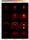 |
Fig. 3 Synchrotron radio emission maps of grid of models with θobs = 45°. |
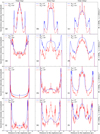 |
Fig. 4 Cut through synchrotron radio emission maps of the grid of models with θobs = 45°, taken along the Ox direction. |
4 Discussion
This section presents the limitation of the method and compares the results with observations.
4.1 Limitations of the models
As already reported in the preceding studies using this numerical approach (see Meyer & Meliani 2022; Meyer et al. 2024a), there are two key caveats inherent to this type of simulation. First, it is imperative to understand that the simulations conducted within this study are confined to a two-dimensional framework, assuming axisymmetry, thereby disregarding any potential variations in the supernova progenitor’s axis of rotation or the pulsar’s spin relative to the direction of motion of the massive star or the direction of the ISM magnetic field. This is therefore an exploratory work. While our current approach enhances computational efficiency and provides insights into the supernova remnant problem, only a full three-dimensional treatment would be realistic, permitting, for example, the inclusion of factors such as magnetic turbulence and the multi-phased structure of the ISM, which could profoundly influence the development of the stellar-wind bubble and the expansion of the supernova blast wave. Consequently, it becomes evident that future investigations employing a three-dimensional approach hold the promise of offering a more comprehensive understanding of these complex phenomena. However, the computation cost of such research needs to be downsized before they are deemed possible.
Furthermore, an additional aspect that warrants meticulous consideration is the absence of pulsar motion in the simulations. Integrating pulsar motion into our models would introduce a layer of complexity that is currently absent, thereby affording us a more realistic representation of the intricate interplay between the pulsar wind and its surrounding medium. Moreover, accounting for the oblique rotation of the pulsar’s magnetic axis would facilitate a more accurate reproduction of the observed characteristics of pulsar-wind nebulae, for instance by both non-thermal synchrotron and inverse Compton radiation mechanisms. These aforementioned aspects highlight promising avenues for future research.
It is also important to note that the pulsar itself does not exhaust the possible features of these systems. We assumed a fixed initial spin-down power, a fixed initial period and period derivative, and a fixed wind magnetisation. There is no radiative model incoroporated for the pulsar electron population itself.
4.2 Concluding remarks on emission maps
Taking into account the limitations, the series of emission maps presented in this study cover the parameter space of the most common core-collapse supernova progenitors and explore the most probable bulk velocities reached when animated by a supernova moving through the ISM. Our models therefore measure the deviations from the barrel-to-Cygnus-loop evolutionary sequence, as identified in Meyer et al. (2024b), that are induced by the presence of a pulsar wind blown after the death of the progenitor. A few global remarks can be made. The synchrotron emission maps of the initial 20 M⊙ (red supergiant) progenitor form a bright jet-like feature, which in the case of a high-space- velocity star (v★ = 40 km s−1) is surrounded by a fainter arc embedding the central pulsar-wind nebula. In other words, the pulsar-wind nebula is the brightest component of the supernova remnant. In contrast, for the 35 M⊙ (Wolf-Rayet) progenitor, the surrounding arc resulting from the interaction of the blast wave with the circumstellar medium emits more than the central pulsar-wind nebula, regardless of the inclination angle of the axis of the remnant with respect to the plane of the sky (see Figs. 3, B.1). This implies that an overhanging surrounding shell-like feature around a synchrotron pulsar-wind nebula is a necessary ingredient to identify before associating its progenitor with an initial mass higher than ~20 M⊙.
The cuts taken laterally through the pulsar-wind nebulae show that the models with a progenitor mass of 20 M⊙ (red supergiant) are centrally peaked, especially at later times (>7 kyr), regardless of the inclination of the remnant with respect to the plane of the sky (see Figs. 4b, c, e, and f). When the crosssections are considered along the direction of motion of the progenitor star, two peaks are clearly noticeable if the progenitor mass is 20 M⊙ , except in the early pulsar-wind-nebula formation phase (Fig. C.1d). The situation is more complex and irregular in the case of the supernova remnants generated by a 35M⊙ (Wolf- Rayet) star, in the sense that a single intensity peak forms at the forward shock at the beginning of the pulsar wind expansion, and a second peak forms later. Finally, atypical patterns develop in the context of a fast-moving progenitor (v★ = 40 km s−1), as illustrated in Figs. C.1k, l, making it difficult to identify characteristic synchrotron maps. This is due to the larger cavity shaped by the stellar wind prior to the explosion, inducing a complex reverberation of the shockwave and of the pulsar-wind termination shock.
4.3 Comparison with particular pulsar-wind nebulae
The initial mass function (IMF) of Kroupa (2001) indicates that the distribution of zero-age main-sequence star masses in clusters follows a power-law decrease. This means that most core-collapse supernova progenitors are in the red supergiant phase at the moment of their explosion, while others are in the Wolf-Rayet evolutionary phase (Katsuda et al. 2018). Despite the fact that a significant proportion of Wolf-Rayet stars directly collapse into black holes and generate gravitational waves rather than producing neutron stars (Vink & Harries 2017; Bogomazov et al. 2018), the details of the mechanisms distinguishing these two scenarios are not fully understood (Dessart et al. 2011). The constraint of identifying a supernova progenitor based on its supernova remnant or pulsar-wind nebula is still not possible on a systematic basis (Gal-Yam et al. 2022). However, a few individual pulsar wind nebulae can be directly compared to our simulations.
The Jellyfish nebula around the pulsar B1509–58 in the supernova remnant G320.4–1.2 (MSH 15–52) forms a complex structure that has been studied at various wavelengths. It reveals outflows expanding asymmetrically into a local medium that is, in some regions, of low density. This suggests a governing role of a circumstellar cavity in shaping the pulsar wind nebula (Arendt 1991; Gaensler et al. 2002; Dubner et al. 2002; Abdo et al. 2010; Hu et al. 2022). The discovery of a series of open rings surrounding the pulsar, interpreted as a (potentially reverberating) termination shock (Yatsu et al. 2009), is consistent with our simulations. In the early formation phase of the pulsar wind nebula, its morphology along the direction of motion of the progenitor is round instead of adopting the typical X-shape described by Komissarov & Lyubarsky (2004) (see Figs. 3a, B.1a). This leads us to think that the pre-supernova circumstellar medium of G320.4–1.2 (MSH 15–52) was asymmetric, perhaps induced by the bulk motion of the supernova progenitor through its ambient medium, and that the peculiar morphology of G320.4–1.2 (MSH 15–52) is partly due to this same mechanism that we explore in the present study.
The plerionic supernova remnant N158A and its pulsar B0540–69 (Petre et al. 2007; Lundqvist et al. 2011). N158A is an extraGalactic remnant in the Large Magellanic Cloud with a progenitor mass estimated to be about 20-25 M⊙, although the O and S lines in its enriched environment revealed by X-ray spectrometry suggest a heavier, Wolf-Rayet progenitor (Williams et al. 2008). This may not necessarily be inconsistent, as the zero-age main-sequence mass of Wolf-Rayet stars can be smaller at low metallicity than in the Milky Way (Hainich et al. 2014). It displays a structure made of jet-like and equatorial disc-like features with little evidence of interaction with the surrounding circumstellar medium. This is consistent with the Wolf-Rayet progenitor evolutionary scenario, with a large cavity carved by a powerful wind (see Figs. A.2a, b and A.3a, b).
5 Conclusion
This study explores the effects of a pulsar wind nebula on the shaping of plerionic supernova remnants generated by runaway massive stars, within an explored parameter space corresponding to the most common supernova remnants, both in terms of progenitor mass and bulk motion through the ISM. By means of 2.5 magneto-hydrodynamical simulations (2 dimensions for the scalar quantities plus a toroidal component for the vectors), we first modelled the circumstellar medium of 20 and 35 M⊙ stars moving with velocities 20 and 40 km s−1, in which we deposited the blast wave of a core-collapse supernova remnant (Truelove & McKee 1999). This was followed by the wind of a rotating neutron star (van der Swaluw 2003; Komissarov & Lyubarsky 2004), which advanced from its young to middle-age (12.5 kyr) evolution times (Meyer & Meliani 2022). Within this approach, the direction of motion of the runaway massive star, the direction of the local ambient medium magnetic field assumed to be organised, the rotation axis of the progenitor, and the rotation axis of the pulsar are all aligned. This forces our models to apply to a peculiar class of pulsar wind nebulae, driven by high equatorial energy flux. The progenitors are considered to live and move into the warm phase of the Galactic plane where the background number density amounts to nISM = 0.79 cm−3 for an equilibrium temperature of TISM = 8000 K and where they die and form plerionic remnants. The simulations are performed with the well- tested astrophysical code PLUTO (Mignone et al. 2007, 2012) using the methodology developed for core-collapse supernova remnants (Meyer et al. 2020, 2021b, 2023) and for pulsar-wind nebulae (Meyer & Meliani 2022; Meyer et al. 2024a). The outputs are post-processed for radio synchrotron emission maps to be discussed in the context of real observations (see the studies of Velázquez et al. 2023; Villagran et al. 2024).
Our models show that the distribution of circumstellar material prior to the supernova explosion is relevant to the reverberation of the termination shock of the pulsar-wind nebula (Bandiera et al. 2023a,b), inducing morphologies that deviate from the classical diamond-like solution of Komissarov & Lyubarsky (2004). This is particularly pronounced when the supernova explosion takes place deep in the wind bubble of the progenitor (slowly moving massive star) or when the distribution of a pre-supernova circumstellar medium is particularly dense (high-mass progenitor such as Wolf-Rayet star). Conversely, it is less pronounced when the explosion happens out of the wind bubble, i.e. in the context of a Cygnus Loop remnant (Aschenbach & Leahy 1999) produced by a fast-moving red supergiant star (Brighenti & D’Ercole 1994). Those asymmetric pulsar wind nebulae display a large variety of non-thermal radio-projected emission, either screened by the overhanging interacting supernova blast wave or via projected asymmetric up–down synchrotron emission (Meyer & Meliani 2022). The reverberation of the pulsar reverse shock plays a role in a wider mechanism; that is, the reverberation of the supernova shockwave towards the centre of the explosion. The pulsar wind prevents it from happening entirely and limits the back-and-forth reflection of core-collapse blast waves inside their progenitor’s circumstellar medium (Dwarkadas & Dewey 2013; Fang et al. 2017). This process must have important consequences on the mixing of materials inside of plerionic supernova remnants, which we hope to investigate in the future. Another aspect that we are currently addressing is the development of full threedimensional simulations. These models will better account for magneto-hydrodynamic processes, such as the instabilities that significantly influence the dynamics and morphology of the flow.
Particularly, the question of the jet originating from a moving pulsar and interacting with the circumstellar medium will then be tackled. This will also remove the constraint imposing the alignment of the different rotation axes and direction of motion involved in this problem, greatly enhancing the degree of realism of the models.
Acknowledgements
The author thankfully acknowledges RES resources provided by BSC in MareNostrum to AECT-2024-2-0002. The authors gratefully acknowledge the computing time made available to them on the high-performance computer “Lise” at the NHR Center NHR@ZIB. This center is jointly supported by the Federal Ministry of Education and Research and the state governments participating in the NHR (www.nhr-verein.de/unsere-partner). This work has been supported by the grant PID2021-124581OB-I00 funded by MCIN/AEI/10.13039/501100011033 and 2021SGR00426 of the Generalitat de Catalunya. This work was also supported by the Spanish program Unidad de Excelencia María de Maeztu CEX2020-001058-M. This work also supported by MCIN with funding from European Union NextGeneration EU (PRTR-C17.I1).
Appendix A Density field in the pulsar wind nebulae models
Figures A.1, A.2, and A.3 are the number density fields in our magneto-hydrodynamical simulation of the supernova remnant of the runaway 20 M⊙ star rotating with Ω★/ΩK = 0.1 and moving with velocity v★ = 40 km s−1 (Fig. A.1), of the runaway 35 M⊙ star moving with velocity v★ = 20 km s−1 (Fig. A.2) and of the runaway 35 M⊙ star moving with velocity v★ = 40 km s−1 (Fig. A.3), respectively. The evolution of the plerionic supernova remnant is shown at times 2.5 (a), 5.0 (b), 7.5 (c) and 12.5 kyr (d), respectively. The various black contours highlight the region with a 50% per cent contribution of pulsar-wind material. The black arrows in the right-hand parts of the figures are ISM magnetic field lines.
Appendix B Non-thermal radio emission maps with θ = 0°
Figure B.1 presents the synchrotron radio emission maps of the grid of models with θobs = 0°.
Appendix C Cut along the Oy axis in the non-thermal radio emission maps with θ = 45°
Figure C.1 shows cuts through the Oy axis of the synchrotron radio emission maps of the grid of models with θobs = 45°.
References
- Abdalla, H., Aharonian, F., Ait Benkhali, F., et al. 2021, ApJ, 917, 6 [NASA ADS] [CrossRef] [Google Scholar]
- Abdo, A. A., Ackermann, M., Ajello, M., et al. 2010, ApJ, 714, 927 [NASA ADS] [CrossRef] [Google Scholar]
- Acero, F., Acharyya, A., Adam, R., et al. 2023, Astropart. Phys., 150, 102850 [Google Scholar]
- Aharonian, F., Akhperjanian, A. G., Bazer-Bachi, A. R., et al. 2006, A&A, 457, 899 [NASA ADS] [CrossRef] [EDP Sciences] [Google Scholar]
- Arendt, R. G. 1991, AJ, 101, 2160 [NASA ADS] [CrossRef] [Google Scholar]
- Aschenbach, B., & Leahy, D. A. 1999, A&A, 341, 602 [NASA ADS] [Google Scholar]
- Atoyan, A. M., & Aharonian, F. A. 1996, MNRAS, 278, 525 [NASA ADS] [Google Scholar]
- Baade, W., & Zwicky, F. 1934, Phys. Rev., 46, 76 [NASA ADS] [CrossRef] [Google Scholar]
- Baalmann, L. R., Scherer, K., Fichtner, H., et al. 2020, A&A, 634, A67 [EDP Sciences] [Google Scholar]
- Baalmann, L. R., Scherer, K., Kleimann, J., et al. 2021, A&A, 650, A36 [NASA ADS] [CrossRef] [EDP Sciences] [Google Scholar]
- Bandiera, R., Bucciantini, N., Martín, J., Olmi, B., & Torres, D. F. 2020, MNRAS, 499, 2051 [NASA ADS] [CrossRef] [Google Scholar]
- Bandiera, R., Bucciantini, N., Martín, J., Olmi, B., & Torres, D. F. 2021, MNRAS, 508, 3194 [NASA ADS] [CrossRef] [Google Scholar]
- Bandiera, R., Bucciantini, N., Martín, J., Olmi, B., & Torres, D. F. 2023a, MNRAS, 520, 2451 [NASA ADS] [CrossRef] [Google Scholar]
- Bandiera, R., Bucciantini, N., Olmi, B., & Torres, D. F. 2023b, MNRAS, 525, 2839 [NASA ADS] [CrossRef] [Google Scholar]
- Baranov, V. B., Krasnobaev, K. V., & Onishchenko, O. G. 1975, Sov. Astron. Lett., 1, 81 [Google Scholar]
- Barkov, M. V., Lyutikov, M., & Khangulyan, D. 2019, MNRAS, 484, 4760 [NASA ADS] [CrossRef] [Google Scholar]
- Begelman, M. C. 1998, ApJ, 493, 291 [NASA ADS] [CrossRef] [Google Scholar]
- Begelman, M. C., & Li, Z.-Y. 1992, ApJ, 397, 187 [NASA ADS] [CrossRef] [Google Scholar]
- Blondin, J. M., Chevalier, R. A., & Frierson, D. M. 2001, ApJ, 563, 806 [NASA ADS] [CrossRef] [Google Scholar]
- Bock, D. C. J., Turtle, A. J., & Green, A. J. 1998, AJ, 116, 1886 [NASA ADS] [CrossRef] [Google Scholar]
- Bogomazov, A. I., Cherepashchuk, A. M., Lipunov, V. M., & Tutukov, A. V. 2018, New A, 58, 33 [CrossRef] [Google Scholar]
- Borkowski, K. J., Reynolds, S. P., & Roberts, M. S. E. 2016, ApJ, 819, 160 [NASA ADS] [CrossRef] [Google Scholar]
- Brighenti, F., & D’Ercole, A. 1994, MNRAS, 270, 65 [Google Scholar]
- Brighenti, F., & D’Ercole, A. 1995a, MNRAS, 277, 53 [NASA ADS] [Google Scholar]
- Brighenti, F., & D’Ercole, A. 1995b, MNRAS, 273, 443 [NASA ADS] [CrossRef] [Google Scholar]
- Bucciantini, N. 2018, MNRAS, 478, 2074 [NASA ADS] [CrossRef] [Google Scholar]
- Bucciantini, N., & Bandiera, R. 2001, A&A, 375, 1032 [NASA ADS] [CrossRef] [EDP Sciences] [Google Scholar]
- Bucciantini, N., Bandiera, R., Blondin, J. M., Amato, E., & Del Zanna, L. 2004, A&A, 422, 609 [NASA ADS] [CrossRef] [EDP Sciences] [Google Scholar]
- Bucciantini, N., Arons, J., & Amato, E. 2011, MNRAS, 410, 381 [NASA ADS] [CrossRef] [Google Scholar]
- Bühler, R., & Blandford, R. 2014, Rep. Prog. Phys., 77, 066901 [NASA ADS] [CrossRef] [Google Scholar]
- Camus, N. F., Komissarov, S. S., Bucciantini, N., & Hughes, P. A. 2009, MNRAS, 400, 1241 [CrossRef] [Google Scholar]
- Castro, N., Fossati, L., Hubrig, S., et al. 2015, A&A, 581, A81 [NASA ADS] [EDP Sciences] [Google Scholar]
- Castro, N., Fossati, L., Hubrig, S., et al. 2017, A&A, 597, L6 [NASA ADS] [CrossRef] [EDP Sciences] [Google Scholar]
- Caswell, J. L. 1979, MNRAS, 187, 431 [NASA ADS] [CrossRef] [Google Scholar]
- Chevalier, R. A. 1982, ApJ, 258, 790 [NASA ADS] [CrossRef] [Google Scholar]
- Chevalier, R. A., & Liang, E. P. 1989, ApJ, 344, 332 [NASA ADS] [CrossRef] [Google Scholar]
- Chevalier, R. A., & Luo, D. 1994, ApJ, 421, 225 [NASA ADS] [CrossRef] [Google Scholar]
- Chiotellis, A., Kosenko, D., Schure, K. M., Vink, J., & Kaastra, J. S. 2013, MNRAS, 435, 1659 [NASA ADS] [CrossRef] [Google Scholar]
- Comerón, F., & Kaper, L. 1998, A&A, 338, 273 [Google Scholar]
- Coroniti, F. V. 1990, ApJ, 349, 538 [Google Scholar]
- Coroniti, F. V. 2017, ApJ, 850, 184 [NASA ADS] [CrossRef] [Google Scholar]
- de Vries, M., Romani, R. W., Kargaltsev, O., et al. 2021, ApJ, 908, 50 [NASA ADS] [CrossRef] [Google Scholar]
- Del Zanna, L., Amato, E., & Bucciantini, N. 2004, A&A, 421, 1063 [NASA ADS] [CrossRef] [EDP Sciences] [Google Scholar]
- Del Zanna, L., Volpi, D., Amato, E., & Bucciantini, N. 2006, A&A, 453, 621 [NASA ADS] [CrossRef] [EDP Sciences] [Google Scholar]
- Dessart, L., Hillier, D. J., Livne, E., et al. 2011, MNRAS, 414, 2985 [NASA ADS] [CrossRef] [Google Scholar]
- Driessen, L. N., Domcek, V., Vink, J., et al. 2018, ApJ, 860, 133 [NASA ADS] [CrossRef] [Google Scholar]
- Dubner, G. M., Gaensler, B. M., Giacani, E. B., Goss, W. M., & Green, A. J. 2002, AJ, 123, 337 [NASA ADS] [CrossRef] [Google Scholar]
- Dwarkadas, V. V., & Dewey, D. 2013, High Energy Density Phys., 9, 22 [NASA ADS] [CrossRef] [Google Scholar]
- Ekström, S., Georgy, C., Eggenberger, P., et al. 2012, A&A, 537, A146 [Google Scholar]
- Eldridge, J. J., Genet, F., Daigne, F., & Mochkovitch, R. 2006, MNRAS, 367, 186 [CrossRef] [Google Scholar]
- Fang, J., Yu, H., & Zhang, L. 2017, MNRAS, 464, 940 [NASA ADS] [CrossRef] [Google Scholar]
- Fossati, L., Castro, N., Morel, T., et al. 2015, A&A, 574, A20 [NASA ADS] [CrossRef] [EDP Sciences] [Google Scholar]
- Gabler, M., Wongwathanarat, A., & Janka, H.-T. 2021, MNRAS, 502, 3264 [CrossRef] [Google Scholar]
- Gaensler, B. M., & Slane, P. O. 2006, ARA&A, 44, 17 [Google Scholar]
- Gaensler, B. M., Arons, J., Pivovaroff, M. J., & Kaspi, V. M. 2002, ASP Conf. Ser., 271, 175 [NASA ADS] [Google Scholar]
- Gal-Yam, A., Bruch, R., Schulze, S., et al. 2022, Nature, 601, 201 [NASA ADS] [CrossRef] [Google Scholar]
- Gelfand, J. D., Slane, P. O., & Zhang, W. 2009, ApJ, 703, 2051 [NASA ADS] [CrossRef] [Google Scholar]
- Groh, J. H., Meynet, G., Ekström, S., & Georgy, C. 2014, A&A, 564, A30 [NASA ADS] [CrossRef] [EDP Sciences] [Google Scholar]
- H.E.S.S. Collaboration (Abdalla, H., et al.) 2019, A&A, 627, A100 [NASA ADS] [CrossRef] [EDP Sciences] [Google Scholar]
- Hainich, R., Rühling, U., Todt, H., et al. 2014, A&A, 565, A27 [NASA ADS] [CrossRef] [EDP Sciences] [Google Scholar]
- Harten, A., Lax, P. D., & van Leer, B. 1983, SIAM Review, 25, 35 [CrossRef] [Google Scholar]
- Herbst, K., Scherer, K., Ferreira, S. E. S., et al. 2020, ApJ, 897, L27 [NASA ADS] [CrossRef] [Google Scholar]
- Hester, J. J. 2008, ARA&A, 46, 127 [Google Scholar]
- Hu, C.-P., Ishizaki, W., Ng, C. Y., Tanaka, S. J., & Mong, Y. L. 2022, ApJ, 927, 87 [NASA ADS] [CrossRef] [Google Scholar]
- Kargaltsev, O., Pavlov, G. G., Klingler, N., & Rangelov, B. 2017, J. Plasma Phys., 83, 635830501 [NASA ADS] [CrossRef] [Google Scholar]
- Katsuda, S., Takiwaki, T., Tominaga, N., Moriya, T. J., & Nakamura, K. 2018, ApJ, 863, 127 [Google Scholar]
- Kennel, C. F., & Coroniti, F. V. 1984, ApJ, 283, 710 [Google Scholar]
- Kervella, P., Decin, L., Richards, A. M. S., et al. 2018, A&A, 609, A67 [NASA ADS] [CrossRef] [EDP Sciences] [Google Scholar]
- Kolb, C., Blondin, J., Slane, P., & Temim, T. 2017, ApJ, 844, 1 [CrossRef] [Google Scholar]
- Komissarov, S. S. 2006, MNRAS, 367, 19 [Google Scholar]
- Komissarov, S. S., & Lyubarsky, Y. E. 2003, MNRAS, 344, L93 [NASA ADS] [CrossRef] [Google Scholar]
- Komissarov, S. S., & Lyubarsky, Y. E. 2004, MNRAS, 349, 779 [NASA ADS] [CrossRef] [Google Scholar]
- Komissarov, S. S., & Lyutikov, M. 2011, MNRAS, 414, 2017 [NASA ADS] [CrossRef] [Google Scholar]
- Kotake, K. 2013, Comptes Rendus Physique, 14, 318 [NASA ADS] [CrossRef] [Google Scholar]
- Kotake, K., Takiwaki, T., Suwa, Y., et al. 2012, Adv. Astron., 2012, 428757 [CrossRef] [Google Scholar]
- Kroupa, P. 2001, MNRAS, 322, 231 [NASA ADS] [CrossRef] [Google Scholar]
- Kulkarni, S. R., & Hester, J. J. 1988, Nature, 335, 801 [CrossRef] [Google Scholar]
- Kuroda, T., Kotake, K., & Takiwaki, T. 2012, ApJ, 755, 11 [NASA ADS] [CrossRef] [Google Scholar]
- Lhaaso Collaboration (Cao, Z., et al.) 2021, Science, 373, 425 [Google Scholar]
- Lorimer, D. R. 2008, Liv. Rev. Relativ., 11, 8 [NASA ADS] [CrossRef] [Google Scholar]
- Lundqvist, N., Lundqvist, P., Björnsson, C. I., et al. 2011, MNRAS, 413, 611 [NASA ADS] [CrossRef] [Google Scholar]
- Manchester, R. N., Hobbs, G. B., Teoh, A., & Hobbs, M. 2005, AJ, 129, 1993 [Google Scholar]
- Martin, J., & Torres, D. F. 2022, J. High Energy Astrophys., 36, 128 [CrossRef] [Google Scholar]
- Martin, J., Torres, D. F., & Rea, N. 2012, MNRAS, 427, 415 [NASA ADS] [CrossRef] [Google Scholar]
- Mestre, E., Torres, D. F., de Oña Wilhelmi, E., & Martí, J. 2022, MNRAS, 517, 3550 [NASA ADS] [CrossRef] [Google Scholar]
- Meyer, D. M. A., & Meliani, Z. 2022, MNRAS, 515, L29 [NASA ADS] [CrossRef] [Google Scholar]
- Meyer, D. M.-A., Mackey, J., Langer, N., et al. 2014, MNRAS, 444, 2754 [NASA ADS] [CrossRef] [Google Scholar]
- Meyer, D. M.-A., Langer, N., Mackey, J., Velázquez, P. F., & Gusdorf, A. 2015, MNRAS, 450, 3080 [NASA ADS] [CrossRef] [Google Scholar]
- Meyer, D. M. A., Petrov, M., & Pohl, M. 2020, MNRAS, 493, 3548 [CrossRef] [Google Scholar]
- Meyer, D. M. A., Mignone, A., Petrov, M., et al. 2021a, MNRAS, 506, 5170 [NASA ADS] [CrossRef] [Google Scholar]
- Meyer, D. M. A., Pohl, M., Petrov, M., & Oskinova, L. 2021b, MNRAS, 502, 5340 [NASA ADS] [CrossRef] [Google Scholar]
- Meyer, D. M. A., Pohl, M., Petrov, M., & Egberts, K. 2023, MNRAS, 521, 5354 [NASA ADS] [CrossRef] [Google Scholar]
- Meyer, D. M. A., Meliani, Z., Velázquez, P. F., Pohl, M., & Torres, D. F. 2024a, MNRAS, 527, 5514 [Google Scholar]
- Meyer, D. M. A., Velázquez, P. F., Pohl, M., et al. 2024b, A&A, 687, A127 [NASA ADS] [CrossRef] [EDP Sciences] [Google Scholar]
- Mignone, A., Bodo, G., Massaglia, S., et al. 2007, ApJS, 170, 228 [Google Scholar]
- Mignone, A., Zanni, C., Tzeferacos, P., et al. 2012, ApJS, 198, 7 [Google Scholar]
- Olmi, B., & Bucciantini, N. 2023, PASA, 40, e007 [NASA ADS] [CrossRef] [Google Scholar]
- Olmi, B., Del Zanna, L., Amato, E., Bandiera, R., & Bucciantini, N. 2014, MNRAS, 438, 1518 [NASA ADS] [CrossRef] [Google Scholar]
- Olmi, B., Del Zanna, L., Amato, E., Bucciantini, N., & Mignone, A. 2016, J. Plasma Phys., 82, 635820601 [NASA ADS] [CrossRef] [Google Scholar]
- Orlando, S., Miceli, M., Petruk, O., et al. 2019, A&A, 622, A73 [NASA ADS] [CrossRef] [EDP Sciences] [Google Scholar]
- Orlando, S., Ono, M., Nagataki, S., et al. 2020, A&A, 636, A22 [NASA ADS] [CrossRef] [EDP Sciences] [Google Scholar]
- Orlando, S., Wongwathanarat, A., Janka, H. T., et al. 2021, A&A, 645, A66 [EDP Sciences] [Google Scholar]
- Orlando, S., Wongwathanarat, A., Janka, H. T., et al. 2022, A&A, 666, A2 [NASA ADS] [CrossRef] [EDP Sciences] [Google Scholar]
- Pavan, L., Pühlhofer, G., Bordas, P., et al. 2016, A&A, 591, A91 [NASA ADS] [CrossRef] [EDP Sciences] [Google Scholar]
- Petre, R., Hwang, U., Holt, S. S., Safi-Harb, S., & Williams, R. M. 2007, ApJ, 662, 988 [NASA ADS] [CrossRef] [Google Scholar]
- Popov, M. V., Andrianov, A. S., Burgin, M. S., et al. 2019, Astron. Rep., 63, 391 [NASA ADS] [CrossRef] [Google Scholar]
- Porth, O., Komissarov, S. S., & Keppens, R. 2013, MNRAS, 431, L48 [NASA ADS] [CrossRef] [Google Scholar]
- Porth, O., Komissarov, S. S., & Keppens, R. 2014, MNRAS, 438, 278 [Google Scholar]
- Powell, K. G. 1997, An Approximate Riemann Solver for Magnetohydrodynamics, eds. M. Y. Hussaini, B. van Leer, & J. Van Rosendale (Berlin, Heidelberg: Springer), 570 [Google Scholar]
- Przybilla, N., Fossati, L., Hubrig, S., et al. 2016, A&A, 587, A7 [NASA ADS] [CrossRef] [EDP Sciences] [Google Scholar]
- Rees, M. J., & Gunn, J. E. 1974, MNRAS, 167, 1 [CrossRef] [Google Scholar]
- Reynolds, S. P., & Chevalier, R. A. 1984, ApJ, 278, 630 [CrossRef] [Google Scholar]
- Reynolds, S. P., Pavlov, G. G., Kargaltsev, O., et al. 2017, Space Sci. Rev., 207, 175 [NASA ADS] [CrossRef] [Google Scholar]
- Rozyczka, M., & Franco, J. 1996, ApJ, 469, L127 [Google Scholar]
- Scherer, K., Baalmann, L. R., Fichtner, H., et al. 2020, MNRAS, 493, 4172 [Google Scholar]
- Shibagaki, S., Kuroda, T., Kotake, K., Takiwaki, T., & Fischer, T. 2024, MNRAS, 531, 3732 [NASA ADS] [CrossRef] [Google Scholar]
- Shishkin, D., & Soker, N. 2023, MNRAS, 522, 438 [NASA ADS] [CrossRef] [Google Scholar]
- Slane, P. 2017, in Handbook of Supernovae, eds. A. W. Alsabti, & P. Murdin (Berlin: Springer), 2159 [CrossRef] [Google Scholar]
- Soker, N. 2023a, Res. Astron. Astrophys., 23, 115017 [CrossRef] [Google Scholar]
- Soker, N. 2023b, Res. Astron. Astrophys., 23, 121001 [CrossRef] [Google Scholar]
- Soker, N., & Kaplan, N. 2021, ApJ, 907, 120 [Google Scholar]
- Taylor, J. H., & Weisberg, J. M. 1982, ApJ, 253, 908 [NASA ADS] [CrossRef] [Google Scholar]
- Temim, T., Slane, P., Kolb, C., et al. 2015, ApJ, 808, 100 [CrossRef] [Google Scholar]
- Temim, T., Slane, P., Plucinsky, P. P., et al. 2017, ApJ, 851, 128 [Google Scholar]
- Temim, T., Slane, P., Raymond, J. C., et al. 2022, ApJ, 932, 26 [Google Scholar]
- Toropina, O. D., Romanova, M. M., & Lovelace, R. V. E. 2019, MNRAS, 484, 1475 [CrossRef] [Google Scholar]
- Torres, D. F., Cillis, A., Martín, J., & de Oña Wilhelmi, E. 2014, J. High Energy Astrophys., 1, 31 [NASA ADS] [Google Scholar]
- Truelove, J. K., & McKee, C. F. 1999, ApJS, 120, 299 [Google Scholar]
- van der Swaluw, E. 2003, A&A, 404, 939 [NASA ADS] [CrossRef] [EDP Sciences] [Google Scholar]
- van der Swaluw, E., Achterberg, A., Gallant, Y. A., Downes, T. P., & Keppens, R. 2003, A&A, 397, 913 [NASA ADS] [CrossRef] [EDP Sciences] [Google Scholar]
- van der Swaluw, E., Downes, T. P., & Keegan, R. 2004, A&A, 420, 937 [NASA ADS] [CrossRef] [EDP Sciences] [Google Scholar]
- Velázquez, P. F., Vigh, C. D., Reynoso, E. M., Gómez, D. O., & Schneiter, E. M. 2006, ApJ, 649, 779 [CrossRef] [Google Scholar]
- Velázquez, P. F., Meyer, D. M. A., Chiotellis, A., et al. 2023, MNRAS, 519, 5358 [CrossRef] [Google Scholar]
- Verbunt, F., Igoshev, A., & Cator, E. 2017, A&A, 608, A57 [NASA ADS] [CrossRef] [EDP Sciences] [Google Scholar]
- Villagran, M. A., Gómez, D. O., Velázquez, P. F., et al. 2024, MNRAS, 527, 1601 [Google Scholar]
- Vink, J. S., & Harries, T. J. 2017, A&A, 603, A120 [NASA ADS] [CrossRef] [EDP Sciences] [Google Scholar]
- Vlemmings, W. H. T., Diamond, P. J., & van Langevelde, H. J. 2002, A&A, 394, 589 [NASA ADS] [CrossRef] [EDP Sciences] [Google Scholar]
- Vlemmings, W. H. T., van Langevelde, H. J., & Diamond, P. J. 2005, A&A, 434, 1029 [NASA ADS] [CrossRef] [EDP Sciences] [Google Scholar]
- Weiler, K. W., & Panagia, N. 1980, A&A, 90, 269 [NASA ADS] [Google Scholar]
- Weiler, K. W., & Shaver, P. A. 1978, A&A, 70, 389 [NASA ADS] [Google Scholar]
- Weisskopf, M. C., Tennant, A. F., Arons, J., et al. 2013, ApJ, 765, 56 [NASA ADS] [CrossRef] [Google Scholar]
- Whalen, D., van Veelen, B., O’Shea, B. W., & Norman, M. L. 2008, ApJ, 682, 49 [Google Scholar]
- Wilkin, F. P. 1996, ApJ, 459, L31 [Google Scholar]
- Williams, B. J., Borkowski, K. J., Reynolds, S. P., et al. 2008, ApJ, 687, 1054 [NASA ADS] [CrossRef] [Google Scholar]
- Yatsu, Y., Kawai, N., Shibata, S., & Brinkmann, W. 2009, PASJ, 61, 129 [NASA ADS] [Google Scholar]
Note that the PLUTO code integrates the equations by absorbing a  in the definition of the magnetic field.
We note that this brings additional uncertainty; see the discussion in Bandiera et al. (2021), especially that associated with their Fig. 4. We hope to incorporate this description in the future.
All Tables
All Figures
|
Fig. 1 Temporal evolution (in Myr) of supernova progenitors of zeroage main-sequence 20 M⊙ (dotted red line) and 35 M⊙ (solid blue line) considered in our study. The panels display the stellar mass M★ (panel a, in M⊙), wind velocity vw (panel b, in km s−1 ), and their mass-loss rate Ṁ (panel c; in M⊙ yr−1). |
| In the text | |
|
Fig. 2 Number density fields in our magneto-hydrodynamical simulation of the supernova remnant of the runaway 20 M⊙ star rotating with Ω★/ΩK = 0.1 and moving with velocity v★ = 20 km s−1. The evolution of the plerionic supernova remnant is shown at times 2.5 (a), 5.0 (b), 7.5 (c), and 12.5 kyr (d), respectively. The various black contours highlight the region with a 50% contribution of pulsar-wind material. The black arrows in the right parts of the figures are ISM magnetic field lines. |
| In the text | |
|
Fig. 3 Synchrotron radio emission maps of grid of models with θobs = 45°. |
| In the text | |
|
Fig. 4 Cut through synchrotron radio emission maps of the grid of models with θobs = 45°, taken along the Ox direction. |
| In the text | |
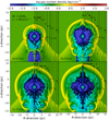 |
Fig. A.1 Same as Fig. 2 but for a 20 M⊙ progenitor star moving with velocity v★ = 40 km s−1. |
| In the text | |
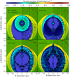 |
Fig. A.2 Same as Fig. 2 but for a 35 M⊙ progenitor star moving with velocity v★ = 20 km s−1. |
| In the text | |
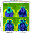 |
Fig. A.3 Same as Fig. 2 but for a 35 M⊙ progenitor star moving with velocity v★ = 40 km s−1. |
| In the text | |
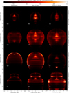 |
Fig. B.1 Same as Fig. 3 but for θobs = 0°. |
| In the text | |
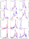 |
Fig. C.1 Same as Fig. 4 but along the Oy direction. |
| In the text | |
Current usage metrics show cumulative count of Article Views (full-text article views including HTML views, PDF and ePub downloads, according to the available data) and Abstracts Views on Vision4Press platform.
Data correspond to usage on the plateform after 2015. The current usage metrics is available 48-96 hours after online publication and is updated daily on week days.
Initial download of the metrics may take a while.