| Issue |
A&A
Volume 691, November 2024
|
|
|---|---|---|
| Article Number | A361 | |
| Number of page(s) | 10 | |
| Section | Stellar atmospheres | |
| DOI | https://doi.org/10.1051/0004-6361/202451878 | |
| Published online | 27 November 2024 | |
Quantitative spectroscopy of multiple OB stars
I. The quadruple system HD 37061 at the centre of Messier 43
Universität Innsbruck, Institut für Astro- und Teilchenphysik,
Technikerstr. 25/8,
6020
Innsbruck,
Austria
★ Corresponding authors; patrick.aschenbrenner@student.uibk.ac.at, norbert.przybilla@uibk.ac.at
Received:
13
August
2024
Accepted:
17
October
2024
Context. The majority of massive stars are located in binary or multiple star systems. Compared to single stars, these objects pose additional challenges to quantitative analyses based on model atmospheres. In particular, little information is currently available on the chemical composition of such systems.
Aims. The members of the quadruple star system HD 37061, which excites the H II region Messier 43 in Orion, are fully characterised. Accurate and precise abundances for all elements with lines traceable in the optical spectrum are derived for the first time.
Methods. A hybrid non-local thermodynamic equilibrium (non-LTE) approach, using line-blanketed hydrostatic model atmospheres computed with the ATLAS12 code in combination with non-LTE line-formation calculations with DETAIL and SURFACE, was employed. A high-resolution composite spectrum was analysed for the atmospheric parameters and elemental abundances of the individual stars. Fundamental stellar parameters were derived based on stellar evolution tracks, and the interstellar reddening was characterised.
Results. We determined the fundamental parameters and chemical abundances for three stars in the HD 37061 system. The fourth and faintest star in the system shows no distinct spectral features, as a result of its fast rotation. However, this star has noticeable effects on the continuum. The derived element abundances and determined ages of the individual stars are consistent with each other, and the abundances coincide with the cosmic abundance standard. We find an excellent agreement between our spectroscopic distance and the Gaia Data Release 3 parallax distance.
Key words: stars: abundances / stars: atmospheres / binaries: spectroscopic / stars: early-type / stars: evolution / stars: fundamental parameters
© The Authors 2024
 Open Access article, published by EDP Sciences, under the terms of the Creative Commons Attribution License (https://creativecommons.org/licenses/by/4.0), which permits unrestricted use, distribution, and reproduction in any medium, provided the original work is properly cited.
This article is published in open access under the Subscribe to Open model. Subscribe to A&A to support open access publication.
1 Introduction
The majority of massive stars, that is, stars with initial masses higher than ~8 M⊙, are situated in binary or multiple star systems (e.g. Chini et al. 2012; Sana et al. 2012). Binary stars are the main sources of fundamental data on stellar masses, M, and radii, R, and are therefore pivotal for the empirical calibration of stellar evolution models. For detached double-lined eclipsing binaries (DEBs) an accuracy of better than ±3% for both M and R can be achieved, as the results rely on only geometry and Newtonian mechanics (Andersen 1991; Torres et al. 2010).
While a number of studies on fundamental stellar parameters are available (see the references in the Andersen and Torres et al. work, as well as more examples of recent work referred to in this paragraph), the knowledge of elemental surface abundances in binary and multiple OB star systems is sparse. This is despite their importance in the context of stellar evolution (tracing mixing processes that can bring nuclear-processed matter to the surface layers) and galactochemical evolution (tracing the chemical homogeneity of stellar environments on small scales and galactic abundance gradients on large scales). Elemental abundances have been routinely determined for (preferentially slowly rotating) single stars or single-lined binary (SB 1) stars (for more recent results, see e.g. Hunter et al. 2009; Nieva & Simón-Díaz 2011; Nieva & Przybilla 2012; Martins et al. 2017; Carneiro et al. 2019; Morel et al. 2022; Blomme et al. 2022; Aschenbrenner et al. 2023). Yet, the composite spectra of double-lined systems (SB2) or even more stars pose additional challenges; as a result, full quantitative spectral analyses of binary or multiple OB stars remain relatively rare. So far, model atmosphere analyses of binaries have been performed on the basis of disentangled spectra from a series of observations (Simon & Sturm 1994; Hadrava 1995), effectively reducing the problem to the standard task of analysing single-star spectra. This encompasses both non-eclipsing (e.g. Mahy et al. 2010; Tkachenko et al. 2016; Raucq et al. 2018; Fabry et al. 2021) and DEB systems (e.g. Pavlovski & Hensberge 2005; Pavlovski & Southworth 2009; Pavlovski et al. 2018, 2023; Johnston et al. 2019). However, the number of chemical elements investigated so far has been restricted to a handful at most, concentrating in particular on C, N, and O to study the effects of mixing in the course of the evolution of the systems’ stars (see in particular Pavlovski et al. 2023).
A different approach, which in principle can be applied to a single-epoch spectrum of a binary or multiple OB star system, was introduced by Irrgang et al. (2014), who studied ten metal species that produce spectral lines in the visual spectrum. Such a single-epoch spectral analysis approach was cross-matched with the analysis of disentangled time-series spectra for a triple star system and a binary with one pulsating component, both of which include one massive magnetic star (González et al. 2017, 2019). What is missing is a more systematic investigation of binary and multiple OB systems, to study to what degree the components share the same abundances (stemming from the same birth cloud) or to what degree chemical peculiarities may develop (e.g. in the presence of a magnetic field).
With the present work, we begin this endeavour, taking advantage of further constraints that have become available over the years from high-angular-resolution observations that use adaptive optics and interferometric techniques as well as Gaia data. Thanks to the many improvements to our analysis methodology that permit an increasingly close reproduction of the optical spectra of OB stars, we intend to provide abundances with uncertainties (1σ standard deviations) smaller than 0.1 dex so that robust conclusions can be drawn.
The object HD 37061 (NU Ori) is the central ionising star of the compact and spherical H II region Messier 43 in Orion. The spectral classification ranges from O9 V (Bragança et al. 2012) to B1 V (Feigelson et al. 2002). We use the modern designation of individual stars by Shultz et al. (2019) in this paper. A close spectroscopic binary was first detected by Morrell & Levato (1991). Based on radial velocity measurements Abt et al. (1991) determined an orbital solution with aperiod of ~19 d (primary designated HD 37061 Aa, the secondary HD 37061 Ab). Later, Preibisch et al. (1999) discovered a second companion at a distance of ~470 mas, designated HD 37061 B. Indications of the presence of a fourth star in the system were found by Grellmann et al. (2013), and this object was confirmed by GRAVITY Collaboration (2018) at a distance of ~8.6 mas and designated HD 37061 C.
Over the past few decades, HD 37061 has attracted interest mostly as a bright background source used to study the interstellar medium (ISM) along an interesting line of sight. Quantitative spectroscopy of HD 37061 has rarely been performed. Simón-Díaz et al. (2011) analysed an intermediate-resolution spectrum, investigating hydrogen and helium lines and accounting only for the primary star. A detailed determination of the orbital elements and fundamental parameters of the three innermost stars was made by Shultz et al. (2019). They used radial velocity measurements from high-resolution spectra and find orbital periods of ~14 d and ~476 d, respectively. The star HD 37061 C is identified as the magnetic star of the system in that work. The chemical composition of the system’s stars has not yet been determined.
The paper is structured as follows. Observations and data reduction are presented in Sect. 2. A description of our models and applied methods is given in Sect. 3. The individual steps of our quantitative analysis are summarised in Sect. 4, and the results, including for the first time a chemical analysis of the system, are discussed in Sect. 5. Finally, we give a summary in Sect. 6. Appendix A shows fits to the spectrum of HD 37061.
2 Observations and data reduction
The analysis is based on high-resolution spectra observed with the Echelle Spectro-Polarimetric Device for the Observation of Stars (ESPaDOnS, Manset & Donati 2003) on the 3.6m Canada-France-Hawaii Telescope (CFHT) on Mauna Kea in Hawaii. The spectra cover a wavelength range from 3700 to 10 500 Å at a resolving power of R = λ/∆λ ≈ 68 000. We used pipeline-reduced spectra downloaded from the CFHT Science Archive at the Canadian Astronomy Data Centre1. The spectra were normalised by fitting a spline function through carefully selected continuum points. We co-added three spectra observed within 2.5 hours on March 8, 2007, to achieve a signal-to-noise ratio (S/N) of 800, measured at ~5100 Å. In addition, various (spectrophotometric) data were used. Low-dispersion, large-aperture spectra taken with the International Ultraviolet Explorer (IUE; see Table 1) were downloaded from the Mikulski Archive for Space Telescopes (MAST2). The short-wavelength (SW) data cover the range λλ1150–1978 Å and the long-wavelength (LW) data λλ1851–3347Å. The IUE spectrophotometric data were co-added to increase the S/N. We note that the radial velocity variations of the spectrum have no effect on the continuum shape, which is later employed to investigate the spectral energy distribution (SED).
IUE spectrophotometry used in the present work.
Model atoms for non-LTE calculations with DETAIL.
3 Model atmospheres and spectrum synthesis
3.1 Models and programs
The analysis is based on a hybrid non-local thermodynamic equilibrium (non-LTE) approach. We employed non-LTE line-formation calculations with the updated and extended versions of the codes DETAIL and SURFACE (Giddings 1981; Butler & Giddings 1985) based on LTE model atmospheres, computed with the ATLAS9/ATLAS 12 codes (Kurucz 1993, 2005). A detailed description is provided by Aschenbrenner et al. (2023). We adopted state-of-the-art model atoms; in Table 2, for each element, the ions considered are listed along with the number of explicit terms (plus superlevels), radiative bound-bound transitions, and references. All model atoms are completed by the ground term of the next-highest ionisation stage (this is not indicated in the table).
Most of the model atoms have been used in other studies. We note that the model atom for O II/III, which was briefly introduced by Aschenbrenner et al. (2023), was slightly extended for the present work, with a 2s2 2p2(1D)4fH 2[5]º term added to O II. In addition, new models for N III/IV were assembled. In summary, the level energies for both ions were adopted from Moore (1993). They were combined into 47 LS-coupled (Russell-Saunders coupling) doublet and quartet terms up to the principal quantum number n = 7 for N III, with the levels for n =8, 9, and 10 combined into three superlevels. The same strategy was followed for N IV, which yielded 84 LS-coupled singlet and triplet terms, and three superlevels for n = 8, 9, and 10 in each spin system. The oscillator strengths and photoionisation cross-sections were for the most part adopted from the Opacity Project (OP, e.g. Seaton et al. 1994), with the data described by Fernley et al. (1999) for N III and Tully et al. (1990) for N IV. Some improved oscillator strengths were taken from Wiese et al. (1996) and Froese Fischer & Tachiev (2004). Photoionisation data missing in the OP were treated as hydrogenic. Electron impact-excitation data for a large number of transitions were adopted from the ab initio calculations of Liang et al. (2012) for N III and of Fernández-Menchero et al. (2017) for N IV. Missing data were calculated using Van Regemorter’s formula (van Regemorter 1962) for radiatively permitted transitions or Allen’s formula (Allen 1973) for forbidden transitions. All collisional ionisation data were calculated via the Seaton formula (Seaton 1962), using OP photoionisation threshold cross-sections or hydrogenic values. For the spectrum synthesis of N III/IV with SURFACE, we employed oscillator strengths taken from calculations based on the multi-configuration Hartree–Fock method (Froese Fischer & Tachiev 2004) and from Kurucz3.
This hybrid non-LTE approach has previously been used to investigate stellar parameters and abundances of a variety of hot stars, with the complexity of the models increasing over the years. Examples encompass slowly rotating single OB main-sequence stars (e.g. Nieva & Przybilla 2007, 2012; Aschenbrenner et al. 2023), massive B-type stars of non-standard chemical composition (e.g. Irrgang et al. 2010, 2022; Przybilla et al. 2021), and massive B-type supergiants (e.g. Weßmayer et al. 2022, 2024). In this work, the method was applied to a multiple massive star system and to faster rotating stars than investigated before.
3.2 Composite spectra
A key part of our analysis is a normalised model spectrum, fcomp, composed of the individual stellar components, to fit the observed spectrum. We generalised Eq. (1) of Irrgang et al. (2014) from binary to multi-star systems:
 (1)
(1)
where fi is the normalised flux of the i-th star, fcont,i the continuum flux of the i-th star, and wi a weight factor corresponding to the effective surface area. Potential binary interactions may also be considered via modifications of the latter.
4 Spectral analysis
We shifted the observed spectrum into the rest frame of the primary star (HD 37061 Aa) by measuring the Doppler shift of the isolated He II, O III, and Si IV lines. In order to fit individual observed spectral lines, we had to include the contribution of all stars simultaneously. To do so, a grid of model spectra was computed for each star, as was done in our previous work on single stars. This allowed us to treat each star individually. We employed self-written Python programs to find the best-fitting grid parameters for all stars by minimising χ2 using the downhill simplex algorithm (Nelder & Mead 1965). At each optimisation step, the free parameters of the model grids were linearly interpolated to get the individual spectra, fi (as well as the continuum fluxes, fcont,i), and then the composite spectrum was created according to Eq. (1). While we could have treated the weights wi as free parameters, we set them to the square radii of the stars.
In addition, a Doppler shift had to be applied to the spectra of the secondary stars. While the Doppler shift for HD 37061 Ab and HD 37061 c can be determined from their absorption lines, the faintest object in the system, HD 37061 B, shows no spectral features, due to its low contributed flux and fast rotation. The object has a separation of 195(4) AU (GRAVITY Collaboration 2018) from the primary. Therefore, we assumed a low orbital velocity and shifted the spectrum of HD 37061 B into the rest frame of the nebula (determined from Hα and the forbidden N II emission lines in the spectrum).
The contributions of the individual components to the formation of the composite spectrum are visualised for a few examples in Fig. 1. Summed up appropriately, these led to a tight fit of the observed spectral features. The effects from neglecting the flux of HD 37061 B are also shown in Fig. 1. The hydrogen lines of the model become slightly too narrow, and the strengths of helium and most metal lines slightly increase. In the red part of the spectrum, we can observe spectral lines where a decent contribution of the line strength apparently stems from HD 37061 B (see the Si II line in Fig. 1).
4.1 Atmospheric parameter and abundance determination
The atmospheric parameters were determined via an analysis of the spectral lines of multiple ionisation stages from nine different chemical species (C, N, O, Ne, Mg, Al, Si, S, and Fe) and an analysis of neutral and single ionised helium lines and the wings of hydrogen Balmer lines. These parameters are the effective temperature, Teff, surface gravity, log 𝑔, helium number fraction, y, microturbulent velocity, ξ, projected rotational velocity, v sin i, and macroturbulence, ζ, as well as the elemental abundances ε (X) = log (X/H) + 12. We derived the parameters on the basis of spectrum synthesis, aiming to simultaneously reproduce detailed line profiles of all stellar components, spanning the entire observed spectral range. An iterative approach was used to overcome ambiguities due to correlations between the parameters of individual stars (e.g. Teff and log g) as well as correlations between the different stars (e.g. element abundances of blended lines), until all parameters were constrained in a single global solution.
4.1.1 Effective temperature and surface gravity
We used different chemical elements and ionisation stages to determine the Teff and log 𝑔 of the individual stars. For HD 37061 Aa, the ionisation equilibria of He I/II, O II/III, and Si III/IV were established as temperature indicators, and the surface gravity was adjusted such that the He II lines were reproduced. This decision was made due to the gravity-sensitive line strength and the single contribution by HD 37061 Aa to the He II lines (see Fig. 1). In the case of HD 37061 Ab, the ionisation equilibria of O I/II and Si II/III were considered as temperature indicators, and the Stark-broadened wings of the hydrogen Balmer lines were used as surface gravity indicators. For HD 37061 C, we used the ionisation equilibria of C II/III and O I/II together with the wings of the hydrogen Balmer lines.
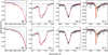 |
Fig. 1 Comparison between the observed spectrum (black) and the synthetic model spectrum (red). The weighted individual contributions of HD 37061 Aa, Ab, B, and C are shown in dotted blue, yellow, magenta, and cyan, respectively. Top row. the model contains the spectral contributions of all four stars. Bottom row. the model excluding the spectral contribution of HD 37061 B. |
4.1.2 Projected rotational velocity and macroturbulence
Both the projected rotational velocity and the macroturbulence were derived simultaneously by fitting the line profiles of isolated metal lines and the wings of blended metal, as well as helium lines. The synthetic models were broadened with rotational and radial-tangential macroturbulence profiles (Gray 2005) and a Gaussian instrumental profile appropriate for the resolving power of the spectrograph.
4.1.3 Microturbulence and elemental abundances
When analysing single-star spectra, the microturbulence is usually adjusted such that the individual line abundances become independent of the line strengths (measured by means of the equivalent width). Since almost all the lines in the spectrum of HD 37061 are blends of the individual stellar components, this is more difficult. Therefore, we instead adjusted the microturbulence such that the variance of the individual line abundances was minimised. Once all of the previously mentioned atmospheric parameters were fixed, we derived the abundance values. First we determined individual line-by-line abundances, and then we calculated the final abundance values and uncertainties as the statistical mean and 1σ standard deviation. In addition to the statistical errors, systematic uncertainties had to be accounted for because of the uncertainties of the atmospheric parameters, the setting of the continuum and the uncertainties of the atomic data used in the non-LTE model atoms. These typically amount to about 0.10–0.15 dex (e.g. Przybilla et al. 2000, 2001b; Nieva & Przybilla 2008) and are likely a bit larger here. This is because we set the microturbulence uncertainty to ± 2 km s−1 as a conservative estimate based on the resolution of our grids, as the number of available lines for determining the abundances, and thus the microturbulence, is more restricted than usual. Modifying the microturbulence within this boundary can change the mean of the derived abundances by ~ 0.1 dex while doubling the (logarithmic) standard deviation.
4.1.4 SED fit
The observed SED was constructed from IUE spectrophotometry as well as Johnson UBV (Ducati 2002) and 2MASS JHK (Cutri et al. 2003) photometry. For the model, we used the ATLAS9 model fluxes of the individual stars, as they can be compared directly with low-resolution observations without any further processing. The model SED is the sum of the individual fluxes, weighted by the squared radii. To account for interstellar extinction, the reddening law of Fitzpatrick (1999) was used, parameterised by the colour excess E(B − V) and the ratio of total-to-selective extinction, RV = AV/E(B – V).
4.2 Fundamental parameters
The stellar evolutionary masses, Mevol, were found by comparing the position of the stars in the spectroscopic Hertzsprung-Russell diagram (sHRD, Langer & Kudritzki 2014) relative to the Geneva evolutionary tracks (Ekström et al. 2012) for rotating stars (v/vcrit = 0.4) at solar metallicity. In the case of the apparently slowly rotating star HD 37061 Ab, we used the Ekström et al. tracks for non-rotating stars. The radii were derived from the definition of the surface gravity 𝑔 = GM/R2, and then the luminosity was derived by applying the Stefan-Boltzmann law  , with σ being the Stefan–Boltzmann constant. Evolutionary ages, τevol, were derived by comparing the star positions with isochrones based on the Ekström et al. tracks.
Stellar parameters of the stars in the HD 37061 system.
4.3 Spectroscopic distances
The stellar flux of an unresolved multi-star system measured at Earth,  , depends on the astrophysical flux emitted at the surface of each star, Fi,λ, and the distance, d, to the system, as well as the individual radii, Ri. The observed magnitude, mX, measured with a normalised filter transmission profile, TX(λ), can then be expressed as
 (2)
(2)
with zp being the zero point of the given filter, X. Defining the synthetic magnitude,  , as
, as
 (3)
(3)
and inserting Eq. (3) into Eq. (2), one can solve for the distance:
 (4)
(4)
In Eq. (4), we rewrote the constants in parsec:  pc. Based on the derived atmospheric parameters, the synthetic magnitude can be calculated from the extinction-corrected (Sect. 4.1.4) predicted flux using Eq. (3). Since the calculated distance depends solely on spectroscopically derived parameters, it is called the spectroscopic distance. In this work we used the dspec derived from the V magnitude.
5 Results
The stellar parameters derived are listed in Table 3: the object’s name, effective temperature, surface gravity, surface helium abundance by number, microturbulence velocity, projected rotational velocity, macroturbulence velocity, colour excess, ratio of total-to-selective extinction, bolometric correction, evolutionary mass, radius, luminosity, evolutionary age, spectroscopic distance (calculated using Eq. (4)), and the Gaia DR3 distance. The object HD 37061 B shows no absorption lines in the spectrum; however, the star has noticeable effects on the continuum. We set Teff and log 𝑔 such that the measured magnitude K = 8.7 mag (GRAVITY Collaboration 2018) is reproduced. Although other parameters cannot be determined, we can conclude that HD 37061 B is a fast-rotating star. Otherwise, absorption lines would be visible (e.g. in the O I λλ7772/74/75 Å triplet). Neglecting the flux contribution of this object would introduce systematic effects to other derived parameters. An increase of ~ 0.05 dex in log 𝑔 would be required for the two other secondary stars to reproduce the wings of the Balmer lines. The analysis of the helium and metal lines would lead to overall slightly lower abundances.
The mean abundances of the chemical elements analysed, the uncertainties and number of spectral lines analysed, and the metallicities are listed in Table 4. While we were able to determine most abundances in the stars, each object is missing one element due to blends or absorption lines that are too weak. The elemental abundances are compatible with each other. They agree within the mutual uncertainties with the cosmic abundance standard (CAS) derived from massive stars in the solar neighbourhood (Nieva & Przybilla 2012; Przybilla et al. 2013), and also with the abundances of the subset of massive stars in Ori OB 1 (Nieva & Simón-Díaz 2011). In particular, the helium abundance of the magnetic star HD 37061 C is consistent with standard values despite its position in the Teff range, where magnetic B stars can show He-strong spectral characteristics (e.g. Smith 1996). The CNO abundances available for the two massive members of HD 37061 are also consistent with pristine values, locating them at the beginning of the path of mixing signatures in the N/O–N/C diagram (Przybilla et al. 2010; Maeder et al. 2014), which is not unexpected for objects that have evolved only slightly from the zero-age main sequence.
We show a comparison between the observed spectrum and our global best-fitting solution in Fig. A.1. The noticeable differences between the model and observations originate mostly from diffuse interstellar bands (DIBs) and telluric absorption due to O2 and H2O in the Earth’s atmosphere. In addition, narrow interstellar absorption lines are visible: the Ca H+K lines, the Na D lines, and the He I λ3889 Å line originating from the metastable 2s 3S level. The spectrum also shows several emission lines from the H II region that surrounds HD 37061: Hα, [N II] λλ6548, 6583 Å, and [S II] λλ6716, 6731 Å. A closer look at selected helium and metal lines is shown in Fig. 2. As a validation of our solution, we included a comparison with an additional spectrum, observed about a year earlier. The relative movement of the individual components from the orbital motion is clearly visible. By changing only the Doppler shifts, we are able to reproduce this observation as well.
Table 4 also includes the nebular abundances of Messier 43 as derived by Simón-Díaz et al. (2011) from collisionally excited lines. The nebular nitrogen abundances agree with the stellar ones. However, nebular oxygen and sulphur appear slightly depleted relative to the stellar abundances. This is likely a consequence of the depletion on dust particles, which means that not all the dust has been destroyed yet, and that the metals have not yet been fully incorporated into the gas phase in the H II region. Some systematic effects can also be expected to affect the nebular abundances, as reflected by the well-known dichotomy of abundances derived from collisionally excited and recombination lines (see, for example, Simón-Díaz & Stasińska 2011 for the case of the Orion nebula, where results from recombination lines required less depletion of metals onto dust).
A fit of the SED, that is, the reproduction of the global energy output of the HD 37061 system, is shown in the upper panel of Fig. 3. As with the detailed spectrum, a tight match is found. However, we were unable to achieve a good fit by varying only RV and E(B – V). We also had to adjust two additional parameters of the Fitzpatrick (1999) reddening law: the UV-bump strength was set to c3 = 2.26 and the far-UV curvature to c4 = 0.20. These values are lower than the average parameters valid for the Milky Way (c3 = 3.23, c4 = 0.41), a situation that can be expected for a sight line that is not dominated by the diffuse ISM but by the material of the remainder of the molecular cloud and the H II region. We also note that the reddening parameters for HD 37061 from Fitzpatrick (1999) match our values within the mutual uncertainties, despite his treatment of HD 37061 as a single star. The findings of Valencic et al. (2004) differ more; in particular, their RV = 4.29 is somewhat smaller than our value, and their c3/RV = 0.31 value is significantly smaller. This could be a consequence of them fitting all eight parameters of the Fitz-patrick reddening law and establishing reddening properties by comparing the observed composite SED of HD 37061 with an un-reddened spectral template of a single star that may have differed from the one employed by Fitzpatrick.
In the lower panel of Fig. 3, we show the positions of the stars analysed in the sHRD (log(ℒ/ℒ⊙) vs log Teff, with  ) based solely on the observed atmospheric parameters. The position of the stars relative to the isochrones and evolutionary tracks suggests that HD 37061 is a young system whose individual stars are coeval. The primary component, HD 37061 Aa, provides the highest sensitivity for the age determination of the system due to its faster evolution. The typical age of the members of the Orion Nebula cluster is widely agreed to be about 1–2 Myr (for an overview, see Muench et al. 2008). Simón-Díaz et al. (2006) derived an age of 2.5±0.5 Myr for the Orion Trapezium stars. Our age determination of
  , Myr is compatible with these values, though somewhat on the high end.
We show a comparison of the stellar parameters of the components of HD 37061 as derived by Shultz et al. (2019) and from the present work in Table 5. There is a remarkable agreement between the values despite the different methods used for their derivation. Shultz et al. used the atmospheric parameters of Simón-Díaz et al. (2011, who analysed HD 37061 as a single star) as a starting point and constrained the physical parameters of the system’s stars using both orbital models and the same evolutionary tracks that we employed here. Our approach relies on spectroscopic analysis, the use of evolutionary models, and some auxiliary data, but not on orbital information. Our systematically slightly larger mass, radius, and luminosity values are a consequence of the slightly larger distance and a slightly higher extinction value we employed. This gives us confidence that future applications of our method can be used to characterise binary and multiple stars with a high degree of confidence from a single spectrum. Time-series spectroscopic investigations are still necessary to derive orbital solutions for such systems, but single-epoch spectra from planned future spectroscopic surveys will no longer need to be discarded from the analysis; they can yield much useful data.
Our solution also allows an update of the inclination angle for HD 37061 C, as the true equatorial rotation velocity can be calculated from the radius and the rotational period, P = 1.09478 (7) d, as determined by Shulz et al. via time-series spectropolarimetry of this magnetic star. It also allows the semi-major axis of the orbit of HD 37061 C around the HD 37061 A binary to be reassessed (see also Table 5).
Metal abundances ε(X) = log(X/H) + 12 (by number) and metallicity, Z (by mass) of the individual objects.
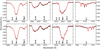 |
Fig. 2 Detailed comparison of the helium and metal lines of the observed spectrum (black) with the global best-fitting solution (red) at different times. The spectra are shifted into the rest frame of the primary star (HD 37061 Aa). The plots in the first column have a different scaled flux axis. Top row: comparison with the spectrum used for the analysis, observed on March 8, 2007. Bottom row: comparison with a spectrum observed on January 12, 2006. The only difference between the models in the top and bottom row is the radial velocity shift of each stellar component. |
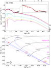 |
Fig. 3 Comparison of the total SED of the HD 37061 system and the location of the individual stars in the sHRD. Upper panel: SED fit of the reddened ATLAS 9 flux (red) to observed UV spectra (black) and photometric measurements (black squares). The inset zooms in on the UV range. The individual contributions of HD 37061 Aa, Ab, B, and C are shown in blue, yellow, magenta, and cyan, respectively. Lower panel: position of the stars in the sHRD. The error ellipses outline 1σ uncertainties; the stars are labelled. Lines of constant log 𝑔 are indicated by dotted magenta lines. The evolutionary tracks of Ekström et al. (2012) for rotating stars (v/vcrit = 0.4) with solar metallicity are overlaid in black. The dash-dotted blue lines are isochrones from Ekström et al. (2012) for log τevol(yr) = 6.0, 6.5, and 7.0. |
Comparison of results from Shultz et al. (2019) and this work.
6 Summary and conclusion
We were able to derive the physical parameters and chemical abundances of three stars in the quadruple system HD 37061. The fourth and faintest star in the system shows no distinct features because of its fast rotation, but contributes noticeable light to the combined continuum of the stars. We modelled the observed composite spectrum by globally fitting the parameters of all stars simultaneously. For the analysis, we assumed that there were no binary interactions because of the stars’ sufficiently large separations, and that each object could therefore be treated as a single star. The combined synthetic spectrum was compared with observations taken about a year apart to verify our approach; we confirm that our approach yielded equally good fits by only varying radial velocities. The derived ages and chemical abundances of the individual stars suggest a common origin and are compatible with typical values for objects in the Orion Nebula region. A fit to the observed SED yielded a good agreement, and our calculated spectroscopic distance based on the derived interstellar extinction curve matches the Gaia distance.
Our results were derived on the basis of a single high-resolution spectrum and are in remarkable agreement with values derived from a spectroscopic time-series analysis that allowed orbital solutions to be obtained and yielded stellar parameters in an independent way (Shultz et al. 2019). This provides confidence for future applications of our method when only single observations are available.
Acknowledgements
The authors are grateful to K. Butler for his advice on atomic data and for many updates and extensions of DETAIL and SURFACE, as well as to A. Irrgang for additional work on the codes. We further thank A. Ebenbichler for provision of a DIB linelist. We also thank our referee, S. Simón-Díaz, for a constructive report that helped to improve the paper. P.A. acknowledges support of this work by grant of a Ph.D. stipend from the Vice Rectorate for Research of the University of Innsbruck. Based on observations obtained at the Canada-France-Hawaii Telescope (CFHT) which is operated by the National Research Council (NRC) of Canada, the Institut National des Sciences de l’Univers of the Centre National de la Recherche Scientifique (CNRS) of France, and the University of Hawaii. The observations at the CFHT were performed with care and respect from the summit of Maunakea which is a significant cultural and historic site.
Appendix A Spectral fit of HD 37061
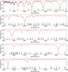 |
Fig. A.1 Comparison between the observed spectrum (black) and the global best fitting model (red). The spectrum is shifted into the rest frame of HD 37061 Aa. Many of the stronger diagnostic lines and diffuse interstellar bands (DIBs) are identified. |
References
- Abt, H. A., Wang, R., & Cardona, O. 1991, ApJ, 367, 155 [NASA ADS] [CrossRef] [Google Scholar]
- Allen, C. W. 1973, Astrophysical Quantities, 3rd edn. (London: Athlone Press) [Google Scholar]
- Andersen, J. 1991, A&A Rev., 3, 91 [Google Scholar]
- Aschenbrenner, P., Przybilla, N., & Butler, K. 2023, A&A, 671, A36 [NASA ADS] [CrossRef] [EDP Sciences] [Google Scholar]
- Becker, S. R. 1998, ASP Conf. Ser., 131, 137 [NASA ADS] [Google Scholar]
- Blomme, R., Daflon, S., Gebran, M., et al. 2022, A&A, 661, A120 [NASA ADS] [CrossRef] [EDP Sciences] [Google Scholar]
- Bragança, G. A., Daflon, S., Cunha, K., et al. 2012, AJ, 144, 130 [CrossRef] [Google Scholar]
- Butler, K., & Giddings, J. R. 1985, Newsletter of Analysis of Astronomical Spectra, 9 (Univ. London) [Google Scholar]
- Carneiro, L. P., Puls, J., Hoffmann, T. L., Holgado, G., & Simón-Díaz, S. 2019, A&A, 623, A3 [NASA ADS] [CrossRef] [EDP Sciences] [Google Scholar]
- Chini, R., Hoffmeister, V. H., Nasseri, A., Stahl, O., & Zinnecker, H. 2012, MNRAS, 424, 1925 [Google Scholar]
- Cutri, R. M., Skrutskie, M. F., van Dyk, S., et al. 2003, VizieR Online Data Catalog, 2246 [Google Scholar]
- Ducati, J. R. 2002, VizieR Online Data Catalog, 2237 [Google Scholar]
- Ekström, S., Georgy, C., Eggenberger, P., et al. 2012, A&A, 537, A146 [Google Scholar]
- Fabry, M., Hawcroft, C., Frost, A. J., et al. 2021, A&A, 651, A119 [NASA ADS] [CrossRef] [EDP Sciences] [Google Scholar]
- Feigelson, E. D., Broos, P., Gaffney, James A.I., et al. 2002, ApJ, 574, 258 [NASA ADS] [CrossRef] [Google Scholar]
- Fernández-Menchero, L., Zatsarinny, O., & Bartschat, K. 2017, J. Phys. B, 50, 065203 [CrossRef] [Google Scholar]
- Fernley, J. A., Hibbert, A., Kingston, A. E., & Seaton, M. J. 1999, J. Phys. B, 32, 5507 [NASA ADS] [CrossRef] [Google Scholar]
- Fitzpatrick, E. L. 1999, PASP, 111, 63 [Google Scholar]
- Froese Fischer, C., & Tachiev, G. 2004, At. Data and Nucl. Data Tables, 87, 1 [NASA ADS] [CrossRef] [Google Scholar]
- Gaia Collaboration (Prusti, T., et al.) 2016, A&A, 595, A1 [NASA ADS] [CrossRef] [EDP Sciences] [Google Scholar]
- Gaia Collaboration (Vallenari, A., et al.) 2023, A&A, 674, A1 [NASA ADS] [CrossRef] [EDP Sciences] [Google Scholar]
- Giddings, J. R. 1981, PhD thesis, University of London, UK [Google Scholar]
- González, J. F., Hubrig, S., Przybilla, N., et al. 2017, MNRAS, 467, 437 [Google Scholar]
- González, J. F., Briquet, M., Przybilla, N., et al. 2019, A&A, 626, A94 [NASA ADS] [CrossRef] [EDP Sciences] [Google Scholar]
- GRAVITY Collaboration (Karl, M., et al.) 2018, A&A, 620, A116 [NASA ADS] [CrossRef] [EDP Sciences] [Google Scholar]
- Gray, D. F. 2005, The Observation and Analysis of Stellar Photospheres, 3rd edn. (Cambridge: Cambridge University Press) [Google Scholar]
- Grellmann, R., Preibisch, T., Ratzka, T., et al. 2013, A&A, 550, A82 [NASA ADS] [CrossRef] [EDP Sciences] [Google Scholar]
- Hadrava, P. 1995, A&AS, 114, 393 [NASA ADS] [Google Scholar]
- Hunter, I., Brott, I., Langer, N., et al. 2009, A&A, 496, 841 [NASA ADS] [CrossRef] [EDP Sciences] [Google Scholar]
- Irrgang, A., Przybilla, N., Heber, U., Nieva, M. F., & Schuh, S. 2010, ApJ, 711, 138 [Google Scholar]
- Irrgang, A., Przybilla, N., Heber, U., et al. 2014, A&A, 565, A63 [NASA ADS] [CrossRef] [EDP Sciences] [Google Scholar]
- Irrgang, A., Przybilla, N., & Meynet, G. 2022, Nat. Astron., 6, 1414 [NASA ADS] [CrossRef] [Google Scholar]
- Johnston, C., Pavlovski, K., & Tkachenko, A. 2019, A&A, 628, A25 [NASA ADS] [CrossRef] [EDP Sciences] [Google Scholar]
- Kurucz, R. 1993, CD-ROM No. 13 (Cambridge, Mass.: SAO) [Google Scholar]
- Kurucz, R. L. 2005, Mem. Soc. Astron. Ital. Suppl., 8, 14 [Google Scholar]
- Langer, N., & Kudritzki, R. P. 2014, A&A, 564, A52 [NASA ADS] [CrossRef] [EDP Sciences] [Google Scholar]
- Liang, G. Y., Badnell, N. R., & Zhao, G. 2012, A&A, 547, A87 [NASA ADS] [CrossRef] [EDP Sciences] [Google Scholar]
- Maeder, A., Przybilla, N., Nieva, M. F., et al. 2014, A&A, 565, A39 [NASA ADS] [CrossRef] [EDP Sciences] [Google Scholar]
- Mahy, L., Rauw, G., Martins, F., et al. 2010, ApJ, 708, 1537 [NASA ADS] [CrossRef] [Google Scholar]
- Manset, N., & Donati, J.-F. 2003, Proc. SPIE, 4843, 425 [NASA ADS] [CrossRef] [Google Scholar]
- Martins, F., Simón-Díaz, S., Barbá, R. H., Gamen, R. C., & Ekström, S. 2017, A&A, 599, A30 [NASA ADS] [CrossRef] [EDP Sciences] [Google Scholar]
- Moore, C. E. 1993, Tables of Spectra of Hydrogen, Carbon, Nitrogen, and Oxygen Atoms and Ions (Boca Raton, FL: CRC Press) [Google Scholar]
- Morrell, N., & Levato, H. 1991, ApJS, 75, 965 [NASA ADS] [CrossRef] [Google Scholar]
- Morel, T., & Butler, K. 2008, A&A, 487, 307 [NASA ADS] [CrossRef] [EDP Sciences] [Google Scholar]
- Morel, T., Butler, K., Aerts, C., Neiner, C., & Briquet, M. 2006, A&A, 457, 651 [NASA ADS] [CrossRef] [EDP Sciences] [Google Scholar]
- Morel, T., Blazère, A., Semaan, T., et al. 2022, A&A, 665, A108 [NASA ADS] [CrossRef] [EDP Sciences] [Google Scholar]
- Muench, A., Getman, K., Hillenbrand, L., & Preibisch, T. 2008, in Handbook of Star Forming Regions, I, ed. B. Reipurth (San Francisco: ASP), 483 [Google Scholar]
- Nelder, J. A., & Mead, R. 1965, Comput. J., 7, 308 [Google Scholar]
- Nieva, M. F., & Przybilla, N. 2006, ApJ, 639, L39 [NASA ADS] [CrossRef] [Google Scholar]
- Nieva, M. F., & Przybilla, N. 2007, A&A, 467, 295 [NASA ADS] [CrossRef] [EDP Sciences] [Google Scholar]
- Nieva, M. F., & Przybilla, N. 2008, A&A, 481, 199 [NASA ADS] [CrossRef] [EDP Sciences] [Google Scholar]
- Nieva, M. F., & Przybilla, N. 2012, A&A, 539, A143 [NASA ADS] [CrossRef] [EDP Sciences] [Google Scholar]
- Nieva, M. F., & Simón-Díaz, S. 2011, A&A, 532, A2 [CrossRef] [EDP Sciences] [Google Scholar]
- Pavlovski, K., & Hensberge, H. 2005, A&A, 439, 309 [NASA ADS] [CrossRef] [EDP Sciences] [Google Scholar]
- Pavlovski, K., & Southworth, J. 2009, MNRAS, 394, 1519 [NASA ADS] [CrossRef] [Google Scholar]
- Pavlovski, K., Southworth, J., & Tamajo, E. 2018, MNRAS, 481, 3129 [NASA ADS] [Google Scholar]
- Pavlovski, K., Southworth, J., Tkachenko, A., Van Reeth, T., & Tamajo, E. 2023, A&A, 671, A139 [NASA ADS] [CrossRef] [EDP Sciences] [Google Scholar]
- Preibisch, T., Balega, Y., Hofmann, K.-H., Weigelt, G., & Zinnecker, H. 1999, New A, 4, 531 [NASA ADS] [CrossRef] [Google Scholar]
- Przybilla, N. 2005, A&A, 443, 293 [NASA ADS] [CrossRef] [EDP Sciences] [Google Scholar]
- Przybilla, N., & Butler, K. 2001, A&A, 379, 955 [NASA ADS] [CrossRef] [EDP Sciences] [Google Scholar]
- Przybilla, N., & Butler, K. 2004, ApJ, 609, 1181 [NASA ADS] [CrossRef] [Google Scholar]
- Przybilla, N., Butler, K., Becker, S. R., Kudritzki, R. P., & Venn, K. A. 2000, A&A, 359, 1085 [NASA ADS] [Google Scholar]
- Przybilla, N., Butler, K., Becker, S. R., & Kudritzki, R. P. 2001a, A&A, 369, 1009 [CrossRef] [EDP Sciences] [Google Scholar]
- Przybilla, N., Butler, K., & Kudritzki, R. P. 2001b, A&A, 379, 936 [NASA ADS] [CrossRef] [EDP Sciences] [Google Scholar]
- Przybilla, N., Firnstein, M., Nieva, M. F., Meynet, G., & Maeder, A. 2010, A&A, 517, A38 [NASA ADS] [CrossRef] [EDP Sciences] [Google Scholar]
- Przybilla, N., Nieva, M. F., Irrgang, A., & Butler, K. 2013, EAS Publ. Ser., 63, 13 [CrossRef] [EDP Sciences] [Google Scholar]
- Przybilla, N., Fossati, L., & Jeffery, C. S. 2021, A&A, 654, A119 [NASA ADS] [CrossRef] [EDP Sciences] [Google Scholar]
- Raucq, F., Rauw, G., Mahy, L., & Simón-Díaz, S. 2018, A&A, 614, A60 [NASA ADS] [CrossRef] [EDP Sciences] [Google Scholar]
- Sana, H., de Mink, S. E., de Koter, A., et al. 2012, Science, 337, 444 [Google Scholar]
- Seaton, M. J. 1962, in Atomic and Molecular Processes, ed. D. R. Bates (New York: Academic Press), 375 [Google Scholar]
- Seaton, M. J., Yan, Y., Mihalas, D., & Pradhan, A. K. 1994, MNRAS, 266, 805 [NASA ADS] [CrossRef] [Google Scholar]
- Shultz, M., Le Bouquin, J. B., Rivinius, T., et al. 2019, MNRAS, 482, 3950 [NASA ADS] [CrossRef] [Google Scholar]
- Simon, K. P., & Sturm, E. 1994, A&A, 281, 286 [NASA ADS] [Google Scholar]
- Simón-Díaz, S., & Stasinska, G. 2011, A&A, 526, A48 [CrossRef] [EDP Sciences] [Google Scholar]
- Simón-Díaz, S., Herrero, A., Esteban, C., & Najarro, F. 2006, A&A, 448, 351 [NASA ADS] [CrossRef] [EDP Sciences] [Google Scholar]
- Simón-Díaz, S., García-Rojas, J., Esteban, C., et al. 2011, A&A, 530, A57 [NASA ADS] [CrossRef] [EDP Sciences] [Google Scholar]
- Smith, K. C. 1996, Ap&SS, 237, 77 [NASA ADS] [CrossRef] [Google Scholar]
- Tkachenko, A., Matthews, J. M., Aerts, C., et al. 2016, MNRAS, 458, 1964 [NASA ADS] [CrossRef] [Google Scholar]
- Torres, G., Andersen, J., & Giménez, A. 2010, A&A Rev., 18, 67 [Google Scholar]
- Tully, J. A., Seaton, M. J., & Berrington, K. A. 1990, J. Phys. B, 23, 3811 [NASA ADS] [CrossRef] [Google Scholar]
- Valencic, L. A., Clayton, G. C., & Gordon, K. D. 2004, ApJ, 616, 912 [NASA ADS] [CrossRef] [Google Scholar]
- van Regemorter, H. 1962, ApJ, 136, 906 [NASA ADS] [CrossRef] [Google Scholar]
- Vrancken, M., Butler, K., & Becker, S. R. 1996, A&A, 311, 661 [NASA ADS] [Google Scholar]
- Weßmayer, D., Przybilla, N., & Butler, K. 2022, A&A, 668, A92 [NASA ADS] [CrossRef] [EDP Sciences] [Google Scholar]
- Weßmayer, D., Urbaneja, M. A., Butler, K., & Przybilla, N. 2024, A&A, 687, L7 [NASA ADS] [CrossRef] [EDP Sciences] [Google Scholar]
- Wiese, W. L., Fuhr, J. R., & Deters, T. M. 1996, J. Phys. & Chem. Ref. Data, Monograph 7 (Melville, NY: AIP Press) [Google Scholar]
All Tables
Metal abundances ε(X) = log(X/H) + 12 (by number) and metallicity, Z (by mass) of the individual objects.
All Figures
|
Fig. 1 Comparison between the observed spectrum (black) and the synthetic model spectrum (red). The weighted individual contributions of HD 37061 Aa, Ab, B, and C are shown in dotted blue, yellow, magenta, and cyan, respectively. Top row. the model contains the spectral contributions of all four stars. Bottom row. the model excluding the spectral contribution of HD 37061 B. |
| In the text | |
|
Fig. 2 Detailed comparison of the helium and metal lines of the observed spectrum (black) with the global best-fitting solution (red) at different times. The spectra are shifted into the rest frame of the primary star (HD 37061 Aa). The plots in the first column have a different scaled flux axis. Top row: comparison with the spectrum used for the analysis, observed on March 8, 2007. Bottom row: comparison with a spectrum observed on January 12, 2006. The only difference between the models in the top and bottom row is the radial velocity shift of each stellar component. |
| In the text | |
|
Fig. 3 Comparison of the total SED of the HD 37061 system and the location of the individual stars in the sHRD. Upper panel: SED fit of the reddened ATLAS 9 flux (red) to observed UV spectra (black) and photometric measurements (black squares). The inset zooms in on the UV range. The individual contributions of HD 37061 Aa, Ab, B, and C are shown in blue, yellow, magenta, and cyan, respectively. Lower panel: position of the stars in the sHRD. The error ellipses outline 1σ uncertainties; the stars are labelled. Lines of constant log 𝑔 are indicated by dotted magenta lines. The evolutionary tracks of Ekström et al. (2012) for rotating stars (v/vcrit = 0.4) with solar metallicity are overlaid in black. The dash-dotted blue lines are isochrones from Ekström et al. (2012) for log τevol(yr) = 6.0, 6.5, and 7.0. |
| In the text | |
|
Fig. A.1 Comparison between the observed spectrum (black) and the global best fitting model (red). The spectrum is shifted into the rest frame of HD 37061 Aa. Many of the stronger diagnostic lines and diffuse interstellar bands (DIBs) are identified. |
| In the text | |
Current usage metrics show cumulative count of Article Views (full-text article views including HTML views, PDF and ePub downloads, according to the available data) and Abstracts Views on Vision4Press platform.
Data correspond to usage on the plateform after 2015. The current usage metrics is available 48-96 hours after online publication and is updated daily on week days.
Initial download of the metrics may take a while.