| Issue |
A&A
Volume 691, November 2024
|
|
|---|---|---|
| Article Number | A91 | |
| Number of page(s) | 15 | |
| Section | Planets and planetary systems | |
| DOI | https://doi.org/10.1051/0004-6361/202451439 | |
| Published online | 01 November 2024 | |
Auroral 3D structure retrieval from the Juno/UVS data
1
Laboratory for Planetary and Atmospheric Physics, STAR Institute, University of Liège,
Liège,
Belgium
2
The University of Edinburgh, School of GeoSciences,
Edinburgh,
UK
3
Aix-Marseille Université, CNRS, CNES, Institut Origines, LAM,
Marseille,
France
4
Space Science and Engineering Division, Southwest Research Institute,
San Antonio,
TX,
USA
5
NASA Langley Research Center,
Hampton, Va,
USA
6
Science Systems And Applications Inc.,
Hampton, Va,
USA
7
Univ. Grenoble Alpes, CNRS, IPAG,
38000
Grenoble,
France
8
Univ. Grenoble Alpes, CSUG,
38000
Grenoble,
France
9
Jet Propulsion Laboratory, California Institute of Technology,
4800 Oak Grove Drive,
Pasadena,
CA
91109,
USA
10
Institute for Space Astrophysics and Planetology, National Institute for Astrophysics (INAF-IAPS),
Roma,
Italy
11
Space Research Institute (IWF), Austrian Academy of Sciences (ÖAW)
Schmiedlstraße 6,
8042
Graz,
Austria
★ Corresponding author; bilal.benmahi@uliege.be
Received:
9
July
2024
Accepted:
25
September
2024
Context. Jovian auroras, the most powerful in the Solar System, result from the interaction between the magnetosphere and atmosphere of Jupiter. While the horizontal morphology of these phenomena has been widely studied, their vertical structure, determined by the penetration depth of the magnetospheric electron into the auroral regions, remains relatively unexplored. Previous observations, including those from the Hubble Space Telescope (HST), have addressed this question to a limited extent.
Aims. In this study we aim to map the vertical structure of Jovian auroral emissions.
Methods. Using observations from Juno’s UltraViolet Spectrograph (UVS), we examined the vertical structure of the auroral emissions. Building on a recent study of auroral energy mapping based on UVS observations that mapped the average energy of precipitating electrons in the Jovian auroral regions, we find a relationship between this average energy and the volume emission rate (VER) of H2 for two types of electron energy distributions: monoenergetic and a kappa distribution with κ = 2.5.
Results. Using brightness maps, we derived the 3D VER structure of Jovian auroras in both northern and southern regions, across multiple spacecraft perijoves (PJs). By considering the example of PJ11, we find that the average altitude of the VER peak in the polar emission region is approximately ~250 km for the monoenergetic distribution case and ~190 km for kappa distribution case. In the main emission region, we find that the average altitude of the VER peak is approximately ~260 km for the case of monoenergetic distribution and ~197 km for kappa distribution case. For the other PJs, we obtained results that are very similar to those of PJ11.
Conclusions. Our findings are, on average, consistent with measurements from the Galileo probe and the HST observations. This study contributes to a better understanding of the complexity of Jovian auroras and highlights the importance of using Juno observations when probing their vertical structure. Considering the variability in the κ parameter in the auroral region, we also studied the impact of this variability on the vertical structure of the auroral emission. This sensitivity study reveals that the influence of the κ parameter on our results was very weak. However, the impact of the κ variability on the VER amplitude shows that there is an influence on the thermal structure and chemical composition of the atmosphere in the auroral regions.
Key words: plasmas / planets and satellites: atmospheres / planets and satellites: aurorae / planets and satellites: composition / planets and satellites: gaseous planets
© The Authors 2024
 Open Access article, published by EDP Sciences, under the terms of the Creative Commons Attribution License (https://creativecommons.org/licenses/by/4.0), which permits unrestricted use, distribution, and reproduction in any medium, provided the original work is properly cited.
This article is published in open access under the Subscribe to Open model. Subscribe to A&A to support open access publication.
1 Introduction
The interaction of the magnetosphere with the atmosphere through the precipitation of charged particles gives rise to the luminous auroral phenomena. In Jupiter’s atmosphere, particularly in its polar regions, the strength of the planet’s magnetic field and the extent of its magnetosphere generate the most intense and largest auroral phenomena in the Solar System. The Jovian auroral emissions form regular and extensive structures in the northern and southern polar regions of the planet. These auroral regions can be classified into three emission subregions: polar emission, main emission, and outer emission. In these auroral regions, the main emission oval predominates in intensity, while the outer and polar emission regions have average intensities that can be 3 to 10 times weaker.
Jovian auroras are observable primarily in the near- and mid-IR domains and in the extreme- and far-ultraviolet (EUV and FUV) domains (see, e.g., Badman et al. 2015). The IR auroral emissions mainly originate from emissions of the fundamental band, the Q branch lines between 3.9 and 4 μm, from the ro-vibrational transitions of the ![$\[\mathrm{H}_3^{+}\]$](/articles/aa/full_html/2024/11/aa51439-24/aa51439-24-eq1.png) molecule (Drossart et al. 1989; Trafton et al. 1989; Geballe et al. 1993). This molecule is predominantly present at very high altitudes in the ionosphere (Kim et al. 1992) and is primarily produced by rapid molecular reactions and the ionizing interaction of magnetospheric electrons with atmospheric compounds, such as H2. These electrons, precipitating in these regions, also interact with other atmospheric particles via inelastic collisions such as e− + H → H* + e− and
molecule (Drossart et al. 1989; Trafton et al. 1989; Geballe et al. 1993). This molecule is predominantly present at very high altitudes in the ionosphere (Kim et al. 1992) and is primarily produced by rapid molecular reactions and the ionizing interaction of magnetospheric electrons with atmospheric compounds, such as H2. These electrons, precipitating in these regions, also interact with other atmospheric particles via inelastic collisions such as e− + H → H* + e− and ![$\[e^{-}+\mathrm{H}_2 \rightarrow \mathrm{H}_2^*+e^{-}\]$](/articles/aa/full_html/2024/11/aa51439-24/aa51439-24-eq2.png) , which are responsible for auroral emissions in the UV domain. These emissions are mainly populated by emissions from the Lyman-alpha line (Broadfoot et al. 1979; Dols et al. 2000) of atomic hydrogen and by emissions from the Lyman and Werner bands of molecular hydrogen (Gérard et al. 2014; Gustin et al. 2016; Benmahi et al. 2024).
, which are responsible for auroral emissions in the UV domain. These emissions are mainly populated by emissions from the Lyman-alpha line (Broadfoot et al. 1979; Dols et al. 2000) of atomic hydrogen and by emissions from the Lyman and Werner bands of molecular hydrogen (Gérard et al. 2014; Gustin et al. 2016; Benmahi et al. 2024).
In the UV domain, particularly between 125 nm and 170 nm, the emission spectrum of H2 makes it possible to derive the initial energy of electrons precipitating in the auroral regions, by measuring the spectral color ratio (CR) defined as CR = ![$\[\frac{I(155 \mathrm{~nm}-162 \mathrm{~nm})}{I(123 \mathrm{~nm}-130 \mathrm{~nm})}\]$](/articles/aa/full_html/2024/11/aa51439-24/aa51439-24-eq3.png) (Yung et al. 1982; Gustin et al. 2013), where
(Yung et al. 1982; Gustin et al. 2013), where ![$\[I\left(\lambda_{\min }-\lambda_{\max }\right)=\int_{\lambda_{\min }}^{\lambda_{\max }} I_\lambda d \lambda\]$](/articles/aa/full_html/2024/11/aa51439-24/aa51439-24-eq4.png) and Iλ is the flux intensity of the spectrum at a wavelength λ. The intervals [123 nm-130 nm] and [155 nm-162 nm] represent, respectively, a range of wavelengths absorbed by Jupiter’s stratospheric CH4 and the unabsorbed part of the spectrum.
and Iλ is the flux intensity of the spectrum at a wavelength λ. The intervals [123 nm-130 nm] and [155 nm-162 nm] represent, respectively, a range of wavelengths absorbed by Jupiter’s stratospheric CH4 and the unabsorbed part of the spectrum.
This CR allows us to evaluate the absorption of the H2 spectrum by CH4. Thus, for a fixed emission angle, in the interval [123 nm-130 nm], an increase in spectral absorption indicates emission by H2 originating from lower altitudes in the atmosphere. This means that magnetospheric electrons penetrate deeper into the atmosphere before thermalizing, indicating that this electrons are more energetic. Consequently, there is a relationship between the CR and the average energy of electrons precipitating in the auroral regions, denoted CR(⟨E⟩). In the rest of the manuscript, we use the notation CR(E), where E represents the average energy of the precipitating electrons. This relationship allows us to derive the energy of precipitating electrons from observations of the CR. This method has been used in several different studies to derive the average energy of precipitating electrons from spectral observations with the Space Telescope Imaging Spectrograph (STIS) on board the Hubble Space Telescope (HST; e.g., Gustin et al. 2013; Gérard et al. 2014). It has also been used by Benmahi et al. (2024), who were the first to use it together with observations from the Ultraviolet Spectrograph (UVS) on board the Juno spacecraft.
The structure of auroral emission is extended both horizontally and vertically up to altitudes where the volume emission rate (VER) is higher than elsewhere. This is due to the penetration of highly energetic electrons whose energy degradation becomes significant at the end of their trajectory. This increases the probability of interaction and thus also increases the collision rate with atmospheric particles, leading to the excitation of H and H2 compounds.
The vertical structure of auroral emission has been studied and observed multiple times across different wavelength ranges (e.g., Vasavada et al. 1999; Cohen & Clarke 2011; Uno et al. 2014; Bonfond et al. 2015). These previous observations were conducted in the visible (Vasavada et al. 1999), IR (Uno et al. 2014), and UV domains (Gérard et al. 2009; Bonfond et al. 2009, 2015) to measure the altitude of the auroral emission peak in Jupiter’s polar regions. Additionally, the altitudes of auroral emission peaks depend on the wavelength at which the emission process occurs. For example, ![$\[\mathrm{H}_3^{+}\]$](/articles/aa/full_html/2024/11/aa51439-24/aa51439-24-eq5.png) emissions in the IR predominantly result from thermal agitation due to high thermospheric temperatures (Drossart et al. 1989) and from the recombination of
emissions in the IR predominantly result from thermal agitation due to high thermospheric temperatures (Drossart et al. 1989) and from the recombination of ![$\[\mathrm{H}_2^{+}\]$](/articles/aa/full_html/2024/11/aa51439-24/aa51439-24-eq6.png) with H2
with H2 ![$\[\left(\mathrm{H}_2+\mathrm{H}_2^{+} \rightarrow \mathrm{H}_3^{+*}+\mathrm{H}\right)\]$](/articles/aa/full_html/2024/11/aa51439-24/aa51439-24-eq7.png) , whereas H2 emissions in the UV primarily result from inelastic collisions of electrons with atmospheric particles between the upper stratosphere and the thermosphere (Broadfoot et al. 1979).
, whereas H2 emissions in the UV primarily result from inelastic collisions of electrons with atmospheric particles between the upper stratosphere and the thermosphere (Broadfoot et al. 1979).
The results obtained by Bonfond et al. (2015) indicate that the altitude of the average emission peak is below 400 km above the 1-bar pressure level in the main emission regions and around 900 km in the Io footprint region. The average altitude of the emission peak was measured at approximately 250 km in the visible domain (Vasavada et al. 1999) and between 590 and 720 km in the IR domain (Uno et al. 2014) above the 1-bar pressure level. The altitudes of the observed spectral emission peaks vary from study to study. Moreover, due to when the observations were carried out, the regions studied were primarily confined to the planet’s limb; this is a major limitation and does not allow a global understanding of the vertical structure of auroral emissions.
In this manuscript we introduce a different approach to indirectly inferring the vertical structure of Jupiter’s auroral emissions, by utilizing the brightness maps observed by Juno/UVS and the average energy maps derived from the CR maps observed by the same instrument. This method stems directly from the study conducted by Benmahi et al. (2024), which explored the inversion of the average energy of precipitated electrons in the auroral regions from observation maps of the CR.
In the previous observations, the techniques involved observing auroral emissions with spectral bands, including wavelengths absorbed by atmospheric compounds, primarily hydrocarbons. These methods do allow vertical emission profiles to be derived, but including wavelengths that can be absorbed by the atmosphere may lead to the erosion of the measured emission profile, shifting the emission peak of this profile to higher altitudes. With our method, we derive the VER profile, which has the advantage of revealing the structure of the auroral emission before it is absorbed by the hydrocarbons present in Jupiter’s atmosphere.
Modeling the CR (see Benmahi et al. 2024) requires the use of an electron transport model coupled with an auroral emission model based on the de-excitation of H2 molecules. This approach allows us to simultaneously model the vertical profile of the VER as a function of the initial mean energy of the precipitated electrons. Thus, the obtained result establishes a relationship between the VER and the mean energy of precipitated electrons. To model this relationship, we considered two types of electron flux distributions precipitating in the Jovian auroral regions in our electronic transport model: the ideal case of a monoenergetic distribution and a broadband kappa-type electron flux distribution. This kappa distribution, as modeled, is characterized by an average energy and a parameter κ = 2.5, inspired by measurements from the Jupiter Energetic Particle Detector Instrument (JEDI) and Jovian Auroral Distributions Experiment (JADE) instruments on board the Juno spacecraft. Observations from the JADE and JEDI instruments have shown that broadband distributions are very common in auroral regions (Mauk et al. 2020; Allegrini et al. 2020). Before Juno, the prevailing hypotheses suggested that intense quasi-static electric fields were more frequent in Jupiter’s polar regions, leading to an expectation of predominantly monoenergetic distributions (see the review by Bagenal et al. 2017). Consequently, this study aims to illustrate how the inversion of the VER structure changes depending on whether the assumed electron flux distribution is monoenergetic or broadband.
In this paper we begin by outlining both the electron transport model and the UV emission model. Next, we delve into the Juno/UVS observations and elucidate the process of deriving the vertical emission profile from the average energy maps established by Benmahi et al. (2024). We then present our results and a discussion before providing our conclusions. In all the following sections, our altitude grids are referenced to the 1-bar pressure level to facilitate direct comparisons with previous studies.
2 Models
2.1 Electronic transport model (TransPlanet)
The precipitation of electrons into Jupiter’s atmosphere has been modeled using the TransPlanet model (Benmahi 2022; Benne 2023; Benmahi et al. 2024; Benne et al. 2024) developed in collaboration with the Institut de Planétologie et d’Astrophysique de Grenoble (IPAG). This transport code is derived from the Trans* family of codes, which was initially created by Lilensten et al. (1989) and updated by Blelly et al. (1996) to study terrestrial auroral regions. The Trans* code was later diversified for adaptation to several planets in the Solar System and even for exoplanetary cases. The core algorithm has been used in Trans-Mars (Witasse et al. 2002, 2003; Simon et al. 2009; Nicholson et al. 2009), Trans-Venus (Gronoff et al. 2007, 2008), Trans-Titan (Lilensten et al. 2005a,b; Gronoff et al. 2009a,b), Trans-Uranus, Trans-Jupiter (Menager et al. 2010), and more recently TransPlanet, which is a planet-independent model (Benmahi 2022; Benne 2023; Benmahi et al. 2024; Benne et al. 2024). This kinetic model calculates the multi-beam interaction of precipitating electrons with atmospheric particles.
As explained in Benmahi et al. (2024), the modeling work involved combining the TransPlanet code with an auroral emission model for H2 molecules in the UV domain, excited by collisions ![$\[e^{-}+\mathrm{H}_2 \rightarrow \mathrm{H}_2^*+e^{-}\]$](/articles/aa/full_html/2024/11/aa51439-24/aa51439-24-eq8.png) . The coupling between these two models is detailed and explained in Benmahi et al. (2024).
. The coupling between these two models is detailed and explained in Benmahi et al. (2024).
In the present study, we modeled the transport of electrons considering only the magnetospheric electrons precipitation. Secondary electrons resulting from ionization by solar UV radiation are neglected because their penetration capability into Jupiter’s atmosphere is weak and occurs at ~1000 km altitude above the homopause of the considered hydrocarbons, such as CH4, C2H2, or C2H6.
The atmospheric model of the auroral region that we used to model electron transport is described in Grodent et al. (2001) and shown in Fig. 1. This model is 1D and accounts for the dominant neutral species (H, H2, He, and CH4) that predominate in Jupiter’s atmosphere. It extends from the stratosphere at a pressure of about ~1 mbar (altitude of about ~100 km above the 1-bar pressure level) to the upper thermosphere (altitude of about ~2300 km above the 1-bar pressure level) corresponding to a pressure of about ~10−9 mbar. The initial density of thermalized electrons considered in the model is that obtained by Hinson et al. (1998) from radio occultations during the Voyager 2 flyby. Due to the limited data available, the initial electron temperature is assumed to be similar to the temperature of neutral atmosphere.
Moreover, since the atmospheric model used is 1D, we do not account for spatial or temporal variability in the abundance of neutral species in the auroral regions, particularly the horizontal variability of CH4. In this study, we considered a horizontally homogeneous and stable chemical composition throughout Jupiter’s aurora, which likely represents a strong approximation. Thus, given that methane is the main tracer used in this study to model the CR, any variation in its abundance can influence the inversion of the mean energy of the precipitating electrons. Therefore, a sensitivity study, considering the variability of the CH4 homopause in the auroral regions according to Sinclair et al. (2020), was performed to estimate the uncertainty on the inversion of the mean energy of precipitating electrons as a function of the CR. This approach was carried out according to the type of initial energy flux distribution considered (kappa distribution or monoenergetic distribution) for the precipitating electrons in the model.
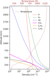 |
Fig. 1 Atmospheric model described by Grodent et al. (2001), which considers only the neutral compounds (H, H2, He, CH4, C2H2, and C2H6) that predominate in Jupiter’s atmosphere. For electronic transport modeling, only H, H2, He, and CH4 compounds were considered. For the UV emission model, spectral absorption by CH4, C2H2, and C2H6 was taken into account. The C2H6 abundance profile is taken from the model from Moses et al. (2005) and Hue et al. (2018). |
2.2 H2 UV emission model
The UV emission model of H2 that we used in this study was developed by Benmahi et al. (2024), drawing inspiration from the models of Dols et al. (2000), Gustin et al. (2002), and Menager (2011). This new emission model is a more optimized version that accounts for nine excited electronic states of H2 (![$\[B^1 \Sigma_u^{+}, C^1 \Pi_u^{+}, C^1 \Pi_u^{-}, B^{\prime 1} \Sigma_u^{+}, B^{\prime \prime 1} \Sigma_u^{+}, D^1 \Pi_u^{+}, D^1 \Pi_u^{-}, D^{\prime 1} \Pi_u^{+}\]$](/articles/aa/full_html/2024/11/aa51439-24/aa51439-24-eq9.png) , and
, and ![$\[D^{\prime 1} \Pi_u^{-}\]$](/articles/aa/full_html/2024/11/aa51439-24/aa51439-24-eq10.png) ), including cascade excitation and self-absorption.
), including cascade excitation and self-absorption.
The spectral emissions of the H2 molecule in the wavelength range [80 nm-190 nm] are primarily populated by rovibrational transitions of the Lyman bands ![$\[\left(B^1 \Sigma_u^{+} \longrightarrow X^1 \Sigma_g^{+}\right)\]$](/articles/aa/full_html/2024/11/aa51439-24/aa51439-24-eq11.png) and Werner bands (
and Werner bands (![$\[C^1 \Pi_u^{+} \rightarrow X^1 \Sigma_g^{+}\]$](/articles/aa/full_html/2024/11/aa51439-24/aa51439-24-eq12.png) and
and ![$\[C^1 \Pi_u^{-} \rightarrow X^1 \Sigma_g^{+}\]$](/articles/aa/full_html/2024/11/aa51439-24/aa51439-24-eq13.png) ). There are also other transitions in the UV spectrum of H2, at shorter wavelengths, originating from the excited levels
). There are also other transitions in the UV spectrum of H2, at shorter wavelengths, originating from the excited levels ![$\[B^{\prime 1} \Sigma_u^{+}, B^{\prime \prime 1} \Sigma_u^{+}, D^1 \Pi_u^{-}, D^1 \Pi_u^{+},D^{\prime} \Pi_u^{-}\]$](/articles/aa/full_html/2024/11/aa51439-24/aa51439-24-eq14.png) , and
, and ![$\[D^{\prime} \Pi_u^{+}\]$](/articles/aa/full_html/2024/11/aa51439-24/aa51439-24-eq15.png) , whose spectral emissions are less intense compared to the Lyman and Werner band emissions and generally fall within the same spectral range. In this study, the UV emission model of H2 in the auroral regions that we used takes into account the excited states B, C, B′, B″, D, and D″, as illustrated here and detailed in Benmahi et al. (2024).
, whose spectral emissions are less intense compared to the Lyman and Werner band emissions and generally fall within the same spectral range. In this study, the UV emission model of H2 in the auroral regions that we used takes into account the excited states B, C, B′, B″, D, and D″, as illustrated here and detailed in Benmahi et al. (2024).
An H2 can be excited to a state nj, vj, and Jj by various processes. It can be excited directly by absorbing a photon, or by collision with an electron or other atmospheric particles. It can also be excited by cascade de-excitation from higher states. Unlike UV auroral emission models of H2 that utilize the Born approximation1 to compute the excitation rates of different excited states (e.g., Waite et al. 1983), in our model, we compute the excitation rates of the considered electronic levels through the energetic flux of electrons calculated by electron transport modeling collisions in Jupiter’s atmosphere. In this model, we also account for the excitation of H2 to the states EF, GK, and ![$\[H \bar{H}\]$](/articles/aa/full_html/2024/11/aa51439-24/aa51439-24-eq16.png) , as well as cascades populating the states B and C. Excitation by other collisional processes with neutral particles is neglected because the atmospheric temperature is not high enough to produce UV emission from collisions of H2 molecules with neutral particles (e.g.,
, as well as cascades populating the states B and C. Excitation by other collisional processes with neutral particles is neglected because the atmospheric temperature is not high enough to produce UV emission from collisions of H2 molecules with neutral particles (e.g., ![$\[\mathrm{H}_2+\mathrm{H}_2=\mathrm{H}_2^*+\mathrm{H}_2\]$](/articles/aa/full_html/2024/11/aa51439-24/aa51439-24-eq17.png) ). Lastly, to account for the auto-absorption phenomenon in the model described here, Benmahi et al. (2024) used the results of Jonin et al. (2000), who experimentally studied the UV spectrum of H2 in the wavelength range [90 nm–120 nm].
). Lastly, to account for the auto-absorption phenomenon in the model described here, Benmahi et al. (2024) used the results of Jonin et al. (2000), who experimentally studied the UV spectrum of H2 in the wavelength range [90 nm–120 nm].
In our UV emission model, we take the absorption by CH4 into account, which primarily absorbs below 140 nm (see Fig. 2). We have also included absorption by C2H2 and C2H6, whose distribution profiles are shown in Fig. 1. The C2H2 abundance profile comes from the model of Grodent et al. (2001). For C2H6, we used the averaged meridional abundance profile from the model of Moses et al. (2005) and Hue et al. (2018). Unlike Gustin et al. (2016) who modified the Moses et al. (2005) C2H6 abundance profile to account for the chemical composition of auroral regions, in our model we simply used the profile of Moses et al. (2005); Hue et al. (2018) because our profile is almost identical to that of Gustin et al. (2016).
C2H2 absorbs primarily in the wavelength range [150 nm-153 nm], as well as in other small wavelength ranges below 140 nm (see Fig. 2). For C2H6, its absorption range is below 157 nm (see Fig. 2). This means that above 145 nm, C2H2 and C2H6 can attenuate the UV emission spectrum. However, below this wavelength, CH4 remains the main absorber of the UV spectrum of H2, and C2H6 absorbs marginally but not negligibly. In this study, to take these absorptions into account, we used the experimentally measured UV cross sections of CH4 (Au et al. 1993; Kameta et al. 2002; Lee et al. 2001), C2H2 and C2H6 (Cooper et al. 1995; Nakayama & Watanabe 2004; Wu et al. 2001).
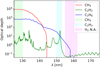 |
Fig. 2 Optical depth calculated over the atmospheric column for CH4, C2H2, and C2H6 and for an emission angle θ = 0°. The transparent green and cyan bands represent the absorption spectral ranges used for the CR calculations. For CH4 the absorption spectral range is considered to be between 125 nm and 130 nm and for C2H2 between 150 nm and 153 nm. The transparent magenta band is the non-absorbed (N.A.) spectral range over which we assume that hydrocarbon absorption is negligible. |
3 Juno/UVS observations
The Juno mission, launched in August 2011, is dedicated to the study of the planet Jupiter and its environment (Bolton et al. 2017). Its insertion into a highly elliptical polar orbit was achieved on July 5, 2016, and its first perijove (PJ) occurred on August 27, 2016. Since then, the probe has completed several dozen PJs, with a periodicity of about 53.5 days during the nominal mission (up to PJ37), allowing close flybys of the polar regions, enabling us to study the interaction between the magnetosphere and the Jovian atmosphere. The probe hosts several scientific instruments, including the UVS. The UVS is specifically designed to study Jupiter’s atmosphere and auroral emissions in the EUV and FUV ranges. Wavelengths ranging from 68 nm to 210 nm are dispersed over a detector with 265 spatial channels × 2048 spectral channels (Davis et al. 2011; Gladstone et al. 2017). The spectrometer slit is dog-bone shaped, parallel to the probe’s rotation axis. This slit has a field of view at the edges of 2° × 0.2° with a theoretical spectral resolution of about 1.9–3.2 nm, and a field of view at the center of 2° × 0.05° with a theoretical spectral resolution of about 1.3 nm (Greathouse et al. 2013). Conversion from counts to brightness units is performed using the numerous stellar observations from UVS (Hue et al. 2019; Hue et al. 2021).
For the present study, we used all the spectral data obtained during PJs 6, 11, 20, 32, 42, and 43. From PJ23 onward, the northern auroral region is increasingly less covered by UVS observations, and the total observing time at the south pole is naturally longer, due to the inclination of Juno’s semimajor axis relative to Jupiter’s equatorial plane. We chose these PJs to have comprehensive northern coverage during the early mission and extensive southern coverage during the most recent PJs (PJ32, PJ42, and PJ43).
Juno is a spin-stabilized probe with a period of about 30 seconds. Consequently, the UVS slit sweeps through the sky and measures the UV emission within its instantaneous field of view, including the emission from Jupiter’s poles (Bonfond et al. 2017). During each 30-second spin period, the UVS field of view intercepts Jupiter. Thus, each point on Jupiter or in the sky that is observed in the wide portion of the slit has an exposure time of approximately ~18 ms during one rotation of the probe, corresponding to the time it takes to pass from one edge of the slit to the other. Auxiliary information is associated with each detected photon, including the x, y (latitude, longitude) coordinates on the UVS detector, the wavelength, and the emission angle relative to the planet. These measured photons are then reorganized into latitude-longitude-wavelength data cubes for each hemisphere. Latitude and longitude are sampled every 1°, and wavelength is sampled every 0.1 nm, corresponding to the instrumental spectral sampling of UVS. Furthermore, to increase the signal-to-noise ratio of the UV emission spectra, we combined the photons measured by the two wide slits of UVS, for which the spectral resolution range from 1.9 to 3.2 nm (Greathouse et al. 2013), and discarded the photons from the narrow slit.
Figure 3 shows the orthographic projection onto the Jupiter’s equatorial plane of the total unabsorbed brightness maps obtained from the UV emission cubes of the northern and southern polar regions for PJ11. To isolate auroral photons from the solar emission backscattered by the Jovian atmosphere, we established a selection criterion for pixels located within the aurora. We selected only the pixels within the region delineated by the Io auroral footpath, recently measured using Juno/UVS by Hue et al. (2023) for the northern and southern auroral regions.
From the data cubes of the PJs we considered in this study, we calculated the spatial distributions of the CR, ![$\[C R=\frac{I(155 \mathrm{~nm}-162 \mathrm{~nm})}{I(125 \mathrm{~nm}-130 \mathrm{~nm})}\]$](/articles/aa/full_html/2024/11/aa51439-24/aa51439-24-eq19.png) , characterizing the absorption of the UV emission spectrum by CH4 and C2H6. It is important to note that we cannot use the canonical wavelength range in the denominator (i.e., 123–130 nm) due to the uncertain calibration caused by the gainloss experienced by Juno/UVS around the Lyman-α line in the region of the wide slit of the detector. Therefore, we started at 125 nm instead. As a result of this different wavelength range, the minimum CR in these maps is about 1.8, which is higher compared to the minimum CR of approximately ~1.1 observed by Gustin et al. (2013), corresponding to an unabsorbed UV emission spectrum. Regarding the maximum CR value, we have a CRmax ≈ 30 according to our spatial sampling for both poles and in the six PJs considered in this study. Polar maps of the CR in the northern and southern hemispheres are presented in Fig. 4 for PJ11.
, characterizing the absorption of the UV emission spectrum by CH4 and C2H6. It is important to note that we cannot use the canonical wavelength range in the denominator (i.e., 123–130 nm) due to the uncertain calibration caused by the gainloss experienced by Juno/UVS around the Lyman-α line in the region of the wide slit of the detector. Therefore, we started at 125 nm instead. As a result of this different wavelength range, the minimum CR in these maps is about 1.8, which is higher compared to the minimum CR of approximately ~1.1 observed by Gustin et al. (2013), corresponding to an unabsorbed UV emission spectrum. Regarding the maximum CR value, we have a CRmax ≈ 30 according to our spatial sampling for both poles and in the six PJs considered in this study. Polar maps of the CR in the northern and southern hemispheres are presented in Fig. 4 for PJ11.
Using the auroral emission model, Benmahi et al. (2024) modeled the relationship linking the CR and the emission angle to the mean energy of electrons precipitating in the Jovian auroral regions (see Figs. D2 and D3 in Benmahi et al. 2024). This relationship, CR(E, θ), was modeled for the case of a kappa energy flux distribution and a monoenergetic energy flux distribution for the precipitating electrons (Benmahi et al. 2024). Thus, by using the CR maps and the emission angles, the mean energy of the electrons precipitating in the northern or southern auroral regions can be inferred. In Figs. 5 and 6, we present the results obtained using this relationship for PJ11.
The mapping of the average energy of precipitating electrons in auroral regions, based on UVS observations, was the subject of the Benmahi et al. (2024) study. The difference between the inverted average energy maps (e.g., Figs. 5 and 6, Benmahi et al. 2024) and the JEDI/JADE measurements of the average energy of the precipitated electrons (e.g., Allegrini et al. 2020) lies in the altitude of the observations. Indeed, using the JADE/JEDI instruments, measurements of electron flux distributions and their average energy are taken at higher altitudes compared to the altitudes where auroral emissions occur, that is to say, they are taken where the electrons deposit most of their energy. Thus, between the altitude where Juno is located and the altitude of auroral emissions, electrons undergo electromagnetic waves interaction that accelerate or decelerate them, thereby altering their average precipitation energy. This is why only an in situ measurement at the top of the atmosphere could precisely provide the average energy of electrons. But measurements at such low altitudes are very rare, even with Juno. However, thanks to the UVS instrument and the presence of hydrocarbons in Jupiter’s atmosphere, this information can be retrieved from the observation of the CR. In this study, or in Benmahi et al. (2024) study, the comparison of the mean energies measured by JADE/JEDI and inverted by UVS is not straightforward, as the temporal resolution of the measurements differs due to the variability of auroral precipitation within these regions. Nevertheless, the comparison of the electrons mean energies inverted from UVS observations with those measured by JEDI (Mauk et al. 2020), on average, are of the same order of magnitude.
In this paper we show and explain our method and results on the inversion of the 3D structure of Jupiter’s auroral emissions, primarily based on PJ11. Results for other PJs will be shown in supplementary materials (see Sect. 6).
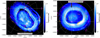 |
Fig. 3 Integrated UV emissions in the [155 nm, 162 nm] range rescaled by a factor of 8.1 to obtain a map of the total unabsorbed emissions from Jupiter’s auroral regions observed during PJ11 in the SIII Jovicentric reference frame. The red arrowed lines represent the solar longitude progression during the observation. The iso-brightening contours have the following values: [1, 10, 100, 500, 1000, 2000] in kR. |
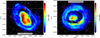 |
Fig. 4 CR of Jupiter’s auroral regions observed during PJ11. In both panels we we show the CR calculated for each pixel of the UV emission map as defined by Gustin et al. (2016) with |
![$\[C R=\frac{I(155 \mathrm{~nm}-162 \mathrm{~nm})}{I(125 \mathrm{~nm}-130 \mathrm{~nm})}\]$](/articles/aa/full_html/2024/11/aa51439-24/aa51439-24-eq18.png)
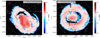 |
Fig. 5 Mean energy maps obtained using the CR(E, θ) relationship modeled for the case of an initial monoenergetic electron flux distribution, and using the CR observed during PJ11 (see Fig. 4) in the north (left panel) and south (right panel) auroral regions. The iso-energy lines have values of 1 keV, 5 keV, and 10 keV, are in steps of 20 keV between 10 keV and 300 keV, and are then in steps of 100 keV between 300 and 900 keV. |
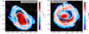 |
Fig. 6 Maps of the inverse average energy for the kappa distribution case. These maps were obtained for the north (left panel) and south (right panel) auroral regions using the CR(E, θ) relationship and the CR observed during PJ11 (see Fig. 4). The iso-energy lines have the same values as in Fig. 5. |
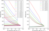 |
Fig. 7 VER vertical profiles modeled for different energies for the case of monoenergetic distribution (left panel) and kappa distribution (right panel). |
4 Method
The CR(E, θ) relationship is obtained directly by modeling the spectral emission of H2 considering a viewing angle θ and an energy flux distribution of electrons characterized by a given mean energy. In this study, we considered two types of energy flux distributions for the electrons precipitating in the auroral regions: a monoenergetic distribution and a kappa distribution (Coumans et al. 2002), which we consider to be representative of the electron flux distributions that precipitate in the auroral regions. To model the CR(E, θ) relationship, we used the same model as Benmahi et al. (2024), which accounts for the absorption of the H2 spectral emission by CH4 and C2H2. However, this time we also considered absorption by C2H6 because its impact on the inversion of the mean energy of precipitating electrons is not negligible and results in a difference of up to 10% with the findings of Benmahi et al. (2024) at higher energies. Therefore, we updated the fit parameters of the phenomenological relationship (see Eq. (D.2) in Benmahi et al. 2024) reproducing CR(E, θ) for each type of electron flux distribution considered in our model. In Appendix B we recall the phenomenological formula in Eq. (B.1) and present the new fit parameter values in Table B.1, which can be used to inverse the mean energies of other PJs from UVS observations.
Each H2 emission spectrum that we modeled was obtained by vertically integrating the modeled VER at each wavelength λ along a given direction θ and accounting for the optical depth of hydrocarbons that absorb these spectral emissions (see Eq. (18) in Benmahi et al. 2024). Thus, by modeling the CR relationship, we simultaneously obtain the vertical profile of the total VER for each mean energy of precipitating electrons in our atmospheric model. This total VER includes the rates of discrete emissions and the rates of continuum emissions for the different electronic states considered in our model in the wavelength range from 80 nm to 170 nm.
In Fig. 7, we present the vertical profiles of the VER as a function of the mean energy E and altitude z for each type of electron energy flux distribution we modeled. By bilinearly interpolating these profiles, we obtained the relations VER(E, z) for each type of electron energy flux distributions considered in this study as shown in Fig. 8. For each modeled mean energy, we considered a constant energy flux Q0 = 1 mWm−2. This allows us to deduce that, with similar flux and mean energy, the maximum of VERκ(z) (for the kappa distribution) is at a lower altitude compared to the maximum of VERmono(z) (for the monoenergetic case). This implies that energetic electrons following a kappa distribution can penetrate deeper into the atmosphere compared to monoenergetic electrons.
Furthermore, in the case of a kappa distribution, the VER profile is broader in altitude, indicating a very extended vertical interaction path of electrons beams with atmospheric particles. These particularities are mainly due to the low-energy electrons in the kappa distribution, which primarily interact at high altitudes, and the very energetic electrons in the tail of this distribution, which penetrate deeply into the atmosphere.
To derive the vertical structure of the observed auroral emissions, we first used the maps of inverted mean energies (shown in Figs. 5 and 6). Thus, in these maps, at each point (x, y) with mean energy Ex,y, and for each type of electron energy flux distribution, we used the modeled relations VERκ(E, z) and VERmono(E, z) presented in Fig. 8 to derive the profiles VERκ(Ex,y,z) and VERmono(Ex,y,z), respectively for the case of a kappa distribution and for the case of a monoenergetic distribution.
Knowing that each derived VER profile at each point (x, y) within the auroral region represents the VER of H2, the total modeled unabsorbed radiance Itot emitted along an emission angle θ is described by the following equation:
![$\[I_{\mathrm{tot}}=\frac{1}{4 \pi \cos (\theta)} \int_0^{\infty} \operatorname{VER}(z) d z \quad\left[\mathrm{~cm}^{-2} \mathrm{~s}^{-1} \mathrm{sr}^{-1}\right].\]$](/articles/aa/full_html/2024/11/aa51439-24/aa51439-24-eq20.png) (1)
(1)
The brightness in Rayleigh (R) is obtained by dividing Itot by ![$\[\frac{1}{4 \pi} \cdot 10^6\]$](/articles/aa/full_html/2024/11/aa51439-24/aa51439-24-eq21.png) [cm−2s−1sr−1].
[cm−2s−1sr−1].
Since the relations of VER(E, z) were obtained considering a constant energy flux Q0, we must account for the actual observed flux at each point (x, y) on the brightness map in a second step. Thus, by vertically integrating each derived profile of VERκ(Ex,y, z) or VERmono(Ex,y,z), we obtain a brightness value, which we divided by the observed brightness at the same (x, y) point to obtain a scaling factor. This factor is applied to the derived VER profile at the same point (x, y) to deduce the final VER profile according to the mean energy and the observed brightness.
To account for emission angles in the relation VER(E, z), we multiplied the observed brightness maps by the cosine of the emission angle maps from the same observation in both hemispheres. This is equivalent to considering that the measured spectral emissions are all zenithal with an emission angle θ = 0°.
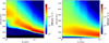 |
Fig. 8 VER as a function of altitude modeled for different energies after bilinear interpolation, for the case of monoenergetic distribution (left panel) and kappa distribution (right panel). |
5 Results and discussion
By applying the method described above, we obtain a 3D structure of the VER in Jupiter’s auroral regions. In our auroral emission model, we considered two types of electron flux distributions precipitating in these regions. Consequently, depending on the considered electron flux distribution, we obtain different auroral emission structures. In Fig. 9 we present the derived structures of the auroral emissions of PJ11 as horizontal slices at different altitudes. The minimum VER value displayed in this figure is 103 cm−3s−1, which, when integrated over a 400 km thick altitude column2, corresponds to a brightness equal to or less than ~20 kR. This lower limit allows us to distinguish the VER structures producing auroral emissions with brightnesses greater than 20 kR.
The derived VER structure in Fig. 9 clearly shows a significant difference between the monoenergetic distribution case and the kappa distribution case. As we gradually increase the altitude of the horizontal slice, the auroral emission rate starts to appear at a significantly lower altitude for the kappa distribution case. For the monoenergetic distribution case, the VER becomes significant starting from about 100 km above the kappa distribution case. This result was expected because the vertical profiles of the VER presented in Fig. 8 show that electrons following a kappa distribution penetrate deeply into Jupiter’s atmosphere.
This inversion of the vertical structure of auroral emissions is a novel result that can serve as a useful tool for future studies and observations. Although the structure of the auroral emission has been derived in a pseudo-3D manner and our electron transport model uses the parallel plane approximation, the configuration of the magnetic field lines, with a median dip magnetic angle of about 65° in the northern auroral region and 74° in the southern one, gives an uncertainty of about ~1000 km on the horizontal spatial position of the derived VER profiles. This uncertainty is comparable to the spatial sampling of the orthographic projection maps presented in the figures of this study.
Regarding the altitude uncertainty in the inversion of the VER vertical profiles, we linearly propagated the uncertainty in the inversion of the mean energies. In fact, by considering the maxima of the CH4 homopause altitudes measured by Sinclair et al. (2020) in the auroral regions, we calculated the upper and lower bounds of the relationship linking the CR to the mean energy of precipitating electrons. Figure 10 shows the evolution of the uncertainty on the inverted mean energy as a function of the CR for the case of a kappa distribution and for the case of a monoenergetic distribution with an emission angle θ = 0°. This result shows that the uncertainty increases with the CR, with an average of about ~100 keV for the kappa distribution case and an average of ~20 keV for the monoenergetic distribution case. By applying these upper and lower bounds to the inversion of the VER profiles for both cases of the electron flux distributions considered in our model, we obtain an average altitude uncertainty of about ~15 km.
In this study, we aimed to compare the results of auroral emission structures by considering only two types of electron flux distributions. Salveter et al. (2022) exploited JADE and JEDI data to measure precipitating electrons along magnetic field lines toward the auroral regions in the main and diffuse emission zones. They showed that in more than 80% of the cases that they considered, the electrons follow a broadband distribution. The remaining 20% are broadband distributions combined with monoenergetic peaks, likely due to electrostatic acceleration processes along the Jovian magnetic field lines. It is well established that, in auroral regions, electron flux distributions vary from one region to another. However, based on the different electron flux distributions measured in the main emission zones by the JADE and JEDI instruments (Salveter et al. 2022), A. Salveter and G. Scicorello estimated that, on average, a broadband kappa distribution with a parameter κ = 2.5 ± 0.4 provides a satisfactory fit for these observations. However, given the variability that the κ parameter can exhibit, particularly in the polar emission regions, we conducted a sensitivity study to understand the impact of this parameter on the vertical structure of auroral emissions (see Appendix A). We conclude that, in general, the variability of the κ parameter does not have a significant impact on the penetration depth of electrons precipitating in auroral regions. Therefore, the kappa distribution with κ = 2.5 that we considered in our study is reasonably representative of electron flux distributions across all auroral regions. However, we observed that the variability of κ influences the amplitude of the VER, which could have a non-negligible impact on the thermal structure and chemical composition in these regions.
Considering the realistic case of a kappa distribution, we notice that, unlike the results obtained with a monoenergetic distribution, the vertical thickness of the auroral curtain seems to be more significant. In the polar emission region, the average vertical thickness of the auroral curtain is about ~250 km for the kappa distribution case. For results obtained considering monoenergetic electrons, the average vertical thickness of the auroral curtain in these same regions is about ~150 km. Similarly, in the main emission regions the auroral curtain obtained for a kappa distribution is thicker, with an average of about ~330 km. For the monoenergetic case, the auroral curtain in these same regions has a thickness of about ~200 km. The average vertical thicknesses of these auroral emissions are similar at both poles for each type of electron flux distribution and for each region.
The vertical thickness of the auroral curtain decreases as the average energy of the precipitating electrons increases. Thus, in the realistic case of a kappa distribution, these curtain thicknesses are consistent with the mean energies we inverted in the northern and southern auroral regions of PJ11. In the polar auroral regions, both north and south, the precipitating electrons are highly energetic. Consequently, the atmospheric vertical thickness in which the majority of the energy deposition occurs is smaller compared to the main emission regions, where the precipitating electrons are 5 to 10 times less energetic. However, the results of the inversion of this auroral structure presented in this section are only valid for PJ11. Other PJs may present different energy configurations. Thus, the vertical dimensions of the auroral emission structure vary over time (see Fig. C1 and Table D1 in the supplementary elements section).
Using the kappa distribution as an example, we can conclude that the primary interaction zone of magnetospheric electrons with Jupiter’s atmosphere is between 150 km (approximately 0.2 mbar pressure relative to the Grodent et al. 2001) and 400 km altitude (approximately 0.3 μbar pressure relative to the Grodent et al. 2001). Although this finding is specific to PJ11, this altitude range is similar for other PJs, except in the polar emission regions where the energy fluctuates significantly from one PJ to another.
At lower altitudes, between 0.01 mbar and 1 mbar, Sinclair et al. (2017) observed temperature peaks in the core of Jupiter’s northern and southern auroral regions, which appear to be associated with auroral activity. While our results on the auroral emission structure were measured a few years apart from Sinclair et al. (2017)’s observations, the altitude range where auroral activity is most intense appears consistent with the pressure levels where temperature peaks are observed. The altitude of the VER peak correlates with that of the electron production rate peak, indicating that the peak of the energy deposition rate by precipitating electrons in the atmosphere occurs at the same altitude. Consequently, it is plausible, according to the energy inversions of Benmahi et al. (2024) of precipitating electrons, that the temperature peaks observed in the upper stratosphere, around 0.2 mbar pressure, are of auroral and thus magnetospheric origin.
Sinclair et al. (2018) also identified peaks in the abundances of major hydrocarbons, such as C2H2 and C2H4, and a trough of abundance of C2H6 within this same altitude range in the Jovian auroral regions. Given the strong electron precipitation in these regions, the abundances of these chemical compounds can be directly influenced by the high production of ![$\[\mathrm{CH}_3^{+}\]$](/articles/aa/full_html/2024/11/aa51439-24/aa51439-24-eq22.png) due to ionization of CH4 by suprathermal electrons (Dobrijevic et al. 2016; Sinclair et al. 2019) or indirectly through the ionization of H2 (Sinclair et al. 2019). Similar to the thermal structure case, the pressure levels where we find (Fig. 9) strong VER seem to align with the observations of Sinclair et al. (2018).
due to ionization of CH4 by suprathermal electrons (Dobrijevic et al. 2016; Sinclair et al. 2019) or indirectly through the ionization of H2 (Sinclair et al. 2019). Similar to the thermal structure case, the pressure levels where we find (Fig. 9) strong VER seem to align with the observations of Sinclair et al. (2018).
To enhance the readability of the inversion of the 3D structure of auroral emissions obtained in our study, we also calculated the altitudes corresponding to the maximum of the derived VER profile at each observed point in the auroral regions. In Figs. 11 and 12, we present these maps for the PJ11 example, respectively for the case of a monoenergetic distribution and for the case of a kappa distribution.
In the case of a monoenergetic electron flux distribution, we find an average altitude of the auroral emission peak of around (250 ± 15) km (corresponding to a pressure of about ~4.5 × 10⁻³ mbar relative to the Grodent et al. 2001) in the polar emission regions. In the main emission regions, the auroral emission peak is located, on average, at an altitude of about (260 ± 15) km (corresponding to a pressure of approximately ~3.5 × 10⁻³ mbar relative to the Grodent et al. 2001). For the kappa distribution, the average altitude of the VER maximum is about (190 ± 15) km (corresponding to a pressure of about ~4 × 10⁻² mbar relative to the Grodent et al. 2001) in the polar emission regions and about (197 ± 15) km in the main emission regions. The observed difference in the emission peak altitudes between the two types of electron flux distributions in our models is due to the energetic electrons in the tail of the kappa distribution penetrating much deeper into the atmosphere. Additionally, the results shown in Fig. 11 demonstrate that, depending on the average energy of the precipitating electrons, our model is comparable to the results of Gustin et al. (2016), who consider Maxwellian and monoenergetic electrons (see Fig. 12 in Gustin et al. 2016). In the same way as for PJ11, we present in Table D.1 (see Sec. 6) a summary of the results for the other PJs treated in this study.
In this study, we also compared our results with the observations of the auroral emission structure presented in the studies by Vasavada et al. (1999), Uno et al. (2014), and Bonfond et al. (2015). These observations involved measuring the structure of the auroral emissions by conducting limb observations of Jupiter at different times. Moreover, these previous measurements concerned narrow, specific, and distinct auroral regions. In contrast, we derived the structure of the auroral emissions integrally in both the northern and southern hemispheres of Jupiter. Therefore, to make these comparisons, we considered that each of the results from the observations by Vasavada et al. (1999), Uno et al. (2014), and Bonfond et al. (2015) is applicable to the entire auroral region, both north and south.
The average altitude of the auroral emission peak in the main emission regions obtained for a realistic electron flux distribution differs from the observations of Vasavada et al. (1999), Uno et al. (2014), and Bonfond et al. (2015), which cover different wavelength ranges (visible, IR, and UV, respectively). Specifically, the observations of Jupiter’s auroral emission structure in the visible range (Vasavada et al. 1999) show that the peak of the main emission in this wavelength range is estimated at approximately 250 km altitude. In contrast, for all PJs, the peak of the main emission that we derived is, on average, about 50 km below the observations of Vasavada et al. (1999). Comparing our results is not straightforward, as the filters used in these observations cover a broad spectral bandwidth ranging from 385 nm to about 1100 nm. Nevertheless, this small altitude difference indicates that our results are somewhat compatible with these observations.
Regarding the observations of IR emissions, ![$\[\mathrm{H}_3^{+}\]$](/articles/aa/full_html/2024/11/aa51439-24/aa51439-24-eq23.png) ions are produced through a rapid cascade process initiated by the photoionization of molecular hydrogen. In auroral regions, H2 ionization is caused not only by solar EUV radiation but also by collisions with energetic precipitating electrons at these latitudes (Johnson et al. 2018). Near the homopause,
ions are produced through a rapid cascade process initiated by the photoionization of molecular hydrogen. In auroral regions, H2 ionization is caused not only by solar EUV radiation but also by collisions with energetic precipitating electrons at these latitudes (Johnson et al. 2018). Near the homopause, ![$\[\mathrm{H}_3^{+}\]$](/articles/aa/full_html/2024/11/aa51439-24/aa51439-24-eq24.png) is destroyed by chemical reactions with hydrocarbons, explaining why the abundance peak of
is destroyed by chemical reactions with hydrocarbons, explaining why the abundance peak of ![$\[\mathrm{H}_3^{+}\]$](/articles/aa/full_html/2024/11/aa51439-24/aa51439-24-eq25.png) remains primarily above an average altitude of 500–600 km (Uno et al. 2014), resulting in an emission peak at very high altitudes (approximately 800 km). IR emissions of H2 have been observed at altitudes similar to those of
remains primarily above an average altitude of 500–600 km (Uno et al. 2014), resulting in an emission peak at very high altitudes (approximately 800 km). IR emissions of H2 have been observed at altitudes similar to those of ![$\[\mathrm{H}_3^{+}\]$](/articles/aa/full_html/2024/11/aa51439-24/aa51439-24-eq26.png) (Uno et al. 2014). These emissions mainly result from excitation by the dissociative recombination of
(Uno et al. 2014). These emissions mainly result from excitation by the dissociative recombination of ![$\[\mathrm{H}_3^{+}\]$](/articles/aa/full_html/2024/11/aa51439-24/aa51439-24-eq27.png) (Cravens 1987; dos Santos et al. 2007). Thus, it is plausible that there is a slight difference between the altitudes of the IR emission peaks of H2 and
(Cravens 1987; dos Santos et al. 2007). Thus, it is plausible that there is a slight difference between the altitudes of the IR emission peaks of H2 and ![$\[\mathrm{H}_3^{+}\]$](/articles/aa/full_html/2024/11/aa51439-24/aa51439-24-eq28.png) due to molecular diffusion and the approximately up to one-hour lifespan of
due to molecular diffusion and the approximately up to one-hour lifespan of ![$\[\mathrm{H}_3^{+}\]$](/articles/aa/full_html/2024/11/aa51439-24/aa51439-24-eq29.png) (Melin & Stallard 2016; Achilleos et al. 1998), which justifies an IR emission peak of H2 around 650 km in altitude. However, in auroral regions, the modeling of energetic electron precipitation shows that the peak electron production rate occurs several hundred kilometers lower and is correlated with the UV VER peak of H2. Consequently, the UV emissions of H2, primarily caused by collisions with suprathermal electrons prevalent at these altitudes, explain why the UV emissions of this chemical compound are lower in altitude compared to its IR emissions.
(Melin & Stallard 2016; Achilleos et al. 1998), which justifies an IR emission peak of H2 around 650 km in altitude. However, in auroral regions, the modeling of energetic electron precipitation shows that the peak electron production rate occurs several hundred kilometers lower and is correlated with the UV VER peak of H2. Consequently, the UV emissions of H2, primarily caused by collisions with suprathermal electrons prevalent at these altitudes, explain why the UV emissions of this chemical compound are lower in altitude compared to its IR emissions.
In the main emission regions, and in the case of a kappa distribution, the average altitude of the VER peak obtained in our study is situated more than 200 km below the observations of Bonfond et al. (2015), who estimated a maximum auroral emission peak altitude of less than 400 km in these same regions. The altitude difference we observed compared to these observations is consistent. The vertical profiles of auroral emissions observed by Bonfond et al. (2015) at Jupiter’s limb are obtained by integrating the radiance along the line of sight using the solar blind channel (SBC) of the Advanced Camera for Surveys (ACS) on board HST. The SBC, with a bandwidth filter ranging from 115 nm to 170 nm, allows imaging of the vertical structure of auroral emissions within this spectral interval, which includes wavelength ranges primarily absorbed by CH4, C2H2, and C2H6. This absorption by these hydrocarbons is more significant below the homopause, located at about 461 km altitude in the auroral regions (Sinclair et al. 2020), and can erode the bottom of the apparent vertical emission profile of H2, potentially increasing the observed peak altitude at the limb.
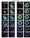 |
Fig. 9 PJ11’s northern and southern auroral emission’s structure sliced at a few different altitudes for the case of monoenergetic distribution (first and third columns) and for the kappa distribution case (second and fourth columns). The delimitation of the main emission region has been defined by Groulard et al. (2024). |
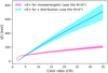 |
Fig. 10 Evolution of the modeled ⟨E⟩ as a function of the CR. The cyan and magenta confidence bands represent the uncertainty on the inverted mean energy, taking the CH4 variability in the auroral regions into account, for the kappa and monoenergetic distribution cases, respectively. In this example, we illustrate the evolution of the uncertainty in the inverted mean energy as a function of the CR for an emission angle θ = 0°. For higher emission angles, the uncertainty follows a similar pattern. |
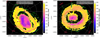 |
Fig. 11 Altitude of the VER maximum maps for the case of monoenergetic distribution in the northern (left panel) and southern (right panel) auroral regions. The delimitation of the main emission region has been defined by Groulard et al. (2024). |
6 Conclusions
Using the auroral emission model developed by Benmahi et al. (2024), we modeled the VER(E, z) relationship for two types of precipitating electron flux distributions in the auroral regions (monoenergetic distribution and kappa distribution). We then combined this relationship with the inverted average energy maps (Benmahi et al. 2024) and the observed brightness maps to derive the 3D structure of Jupiter’s total unabsorbed auroral H2 emission in the UV range [80 nm; 170 nm].
Although the electron distributions in Jovian auroral regions are predominantly of the broadband type (e.g., the ZII regions described by Mauk et al. 2020), they are generally best represented by a kappa distribution. However, in these regions, the kappa parameter can vary slightly, which could alter the shape of the electron flux distribution. To estimate the potential influence of kappa variability on the inversion of the VER structure in our study, we analyzed how sensitively this distribution affected our results. We find that across the different κ values examined in this sensitivity analysis for the same average energy for the precipitated electrons, the altitude of the auroral emission peak remains fairly stable. This stability implies that the altitude is mainly influenced by the average energy of the electron flux distribution in these regions. However, the amplitude of the derived VER(z) profiles varies with different κ values, suggesting that fluctuations in this parameter could impact the thermal structure or chemical composition of the auroral regions. Consequently, in future modeling that integrates the electron transport model with a photochemical model, it will be important to consider the variability of the κ parameter in Jovian auroral zones.
Other types of electron flux distributions precipitating in the auroral regions have also been measured thanks to the observations made by the JEDI instrument (Mauk et al. 2020). These broadband distributions are characterized by the presence of a monoenergetic peak (e.g., the ZI zones described in Mauk et al. 2020), which is probably due to a process of electron acceleration caused by the alignment of the electric field with the magnetic field. This process, also known as the inverted-V acceleration process, seems to occur in very small areas of the magnetosphere. Juno/UVS was able to spatially distinguish these regions in only a few cases (e.g., Sulaiman et al. 2022), but this capability will increase as the mission progresses. In our study, we focused solely on either broadband or monoenergetic distributions and did not take inverted-V acceleration processes into account. Investigating the combined effects of the two types of distributions, along with the range of parameters involved, is beyond the scope of this study. However, for regions with a dominant monoenergetic electron flux distribution, it will be necessary to examine the results, in terms of the mean energy mapping and inversion of the vertical structure of the auroral emission, obtained by considering monoenergetic precipitation in our electron transport model. In the case of broadband distributions, it will be necessary to refer to our kappa distribution results.
The results obtained for the two types of electron flux distributions differ (see Fig. 9). In the case of a monoenergetic distribution, we find a vertical thickness of the auroral curtain of about 150 km in the polar regions and 200 km in the main emission regions. For a kappa distribution, the auroral curtain is thicker, averaging 250 km in the polar regions and about 330 km in the main emission regions. The kappa distribution is more realistic than the monoenergetic distribution for precipitating electrons in Jupiter’s auroral regions (Salveter et al. 2022) and should thus be used in future models to study these regions.
The 3D structure of the auroras can extend higher in altitude, but the method of inverting the average energy of electron precipitation in the auroral regions (Benmahi et al. 2024) is not effective for low-energy electrons. This is because electrons with energies below about 5 keV do not penetrate down into the homopause of CH4 and C2H6, resulting in no absorption in the UV spectrum generated by this type of precipitation.
In the case of the realistic kappa distribution, the altitudes at which there is strong auroral activity are consistent with the altitudes where temperature and hydrocarbon abundance peaks have previously been observed (Sinclair et al. 2017, 2018). This indicates that magnetospheric precipitation influences the chemistry and thermal structure of the auroral regions. We also created maps of the altitudes corresponding to the maximum of the derived VER profile at each observed point in the auroral regions (Figs. 11 and 12). The emission peak altitude measured by Vasavada et al. (1999) appears to be consistent with our results, although the spectral range observed by Vasavada et al. (1999) is much broader.
Our results and the IR observations by Uno et al. (2014) are also compatible. The emissions of H2 and ![$\[\mathrm{H}_3^{+}\]$](/articles/aa/full_html/2024/11/aa51439-24/aa51439-24-eq30.png) in the IR wavelength range have different origins than the UV emissions of H2 and come from higher altitudes (between 650 km and 800 km). Finally, our results are also compatible with the observations of Bonfond et al. (2015), who defined an upper limit of ~400 km for the auroral emission peak altitude of the main emissions in the UV domain.
in the IR wavelength range have different origins than the UV emissions of H2 and come from higher altitudes (between 650 km and 800 km). Finally, our results are also compatible with the observations of Bonfond et al. (2015), who defined an upper limit of ~400 km for the auroral emission peak altitude of the main emissions in the UV domain.
Although the CR(E) method is effective for electrons with energies above 10 keV, there is still uncertainty regarding the variability of hydrocarbon abundance distributions that can influence the CR, such as CH4, C2H2, and C2H6. In this study, we have, for the first time, calculated the uncertainty on the inverted average electron energy considering the variability of CH4 abundance in the auroral regions. However, C2H6 is subject to non-negligible absorption in the [125 nm-130 nm] and [155 nm-157 nm] ranges, which can influence the CR(E) relationship, and this must be taken into account. Measurements of the abundance of this chemical compound in the auroral regions are therefore needed to improve our model.
Data availability
Figure C.1 and Table D.1 are available on Zenodo via https://zenodo.org/records/13847226?token=eyJhbGciOiJIUzUxMiJ9.eyJpZCI6IjE3NzA1ZjdhLTIyOTEtNDFmNy05ZTg1LTZhZTQ3MjI0NzBjMCIsImRhdGEiOnt9LCJyYW5kb20iOiJjYTg4YzI2YjY1ZjY2ZDE0YWNmYjAwYzYxZjk5MzFmNiJ9.mFbFi78bMWvPO6x4Us8RwOoDQz3U-6GWtFdqmxFe1L7BqE67V-Qe5Wt3AvJ_WC7n0q0DIYHAupn08lFq9YrQRg.
Acknowledgements
This work was supported by the University of Liege under Special Funds for Research, IPD-STEMA Programme. VH acknowledges support from the French government under the France 2030 investment plan, as part of the Initiative d’Excellence d’Aix-Marseille Université – A*MIDEX AMX-22-CPJ-04. CSW is supported by the Austrian Science Fund (FWF) 10.55776/P35954. The work of G.G. was supported by the Solar Systems Workings NASA Grant 80NSSC20K1348.
Appendix A Sensitivity study of the kappa distribution parameter changes
In our study, we assumed that the kappa-type electron flux distribution, with a parameter κ = 2.5, is common to all auroral regions. This value of κ = 2.5 ± 0.4 was obtained by fitting only the JEDI measurements of precipitating electron flux in the main emission regions and in the regions of diffuse emissions (Salveter et al. 2022) obtained during the 20 first PJs. Other JEDI observations (Clark et al. 2017) suggest that in polar regions, the precipitating electron flux distributions are of the broadband type, indicating that they can also be represented by a kappa distribution.
However, as we mentioned in this manuscript, the κ parameter can vary slightly from one region to another. Therefore, to assess the impact of this κ parameter on the shape of the vertical structure of auroral emissions, we conducted a sensitivity study. For this, we modeled the VER profile by considering a kappa distribution with an initial precipitation energy flux Q0 = 10mWm−2, an average energy ⟨E⟩ = 50 keV, and different values of κ (κ = 2.001; 2.1; 2.5; 3.0; 5.0; 10).
As a reminder, the kappa-type distribution we considered, Φ(E) ~ fκ(E, ⟨E⟩), characterized by an average energy ⟨E⟩ and a parameter κ governing the logarithmic gradient of the distribution at higher energies, is given by
![$\[f_\kappa(E,\langle E\rangle)=Q_0 \frac{4}{\pi} \frac{\kappa(\kappa-1)}{(\kappa-2)^2} \frac{E}{\langle E\rangle} \frac{\langle E\rangle^{\kappa-1}}{\left(\frac{2 E}{\kappa-2}+\langle E\rangle\right)^{\kappa+1}},\]$](/articles/aa/full_html/2024/11/aa51439-24/aa51439-24-eq31.png) (A.1)
(A.1)
where Q0 represents the total energy flux. The characteristic energy E0, corresponding to the energy at the peak amplitude of the kappa distribution, is related to the average energy ⟨E⟩ by the relation ![$\[\langle E\rangle=2 E_0 \frac{\kappa}{k-2}\]$](/articles/aa/full_html/2024/11/aa51439-24/aa51439-24-eq32.png) .
.
The values of κ chosen for this sensitivity study represent the extreme limits: the lower limit (κ = 2), where the distribution tends to infinity, and the upper limit (κ ≫ 10), where the distribution approaches a Maxwellian distribution. The other values of κ were selected close to the fitted kappa value for this analysis.
Figure A.1 illustrates the shapes of the distributions obtained for each of the chosen values of κ. Figure A.2 presents the different VER(z) profiles obtained after modeling the auroral emission based on the electron precipitation from the various kappa distributions shown in Fig. A.1. For each modeled value of the κ parameter, the altitudes of the VER(z) peak are approximately 197 km, 197 km, 197 km, 217 km, 226 km, and 225 km, respectively. The maximum difference between these altitudes is therefore about 25 km. Given that the estimated uncertainty, considering the variability of the CH4 homopause, on the inversion of the vertical structure of auroral emissions is about 15 km (see Sec. 5), we conclude that for the different κ values considered in this study, the altitude of the auroral emission maximum remains relatively constant. This suggests that this altitude is primarily sensitive to the average energy of the electron flux distribution precipitating in these regions. However, we observe that the different VER(z) profiles show varying amplitudes depending on the values of κ. This indicates that the variability of this parameter can influence the thermal structure or chemical composition of these auroral regions. Moreover, this confirms the analysis by Bonfond et al. (2009) regarding the variation in the altitude of the auroral emission peak based on the assumed shape of the electron distribution. Therefore, in our future modeling efforts that will involve coupling the electron transport model with a photochemical model, it will be necessary to account for the variability of the κ parameter in Jovian auroral regions.
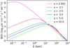 |
Fig. A.1 Examples of kappa electron flux distributions in the energy range [1 eV, 1 MeV] for different values of the κ parameter. These six kappa distributions have the same average energy of 50 keV and the same initial energy flux Q0 = 10mWm−2. The different κ parameters chosen for each distribution are displayed in the legend. |
Appendix B Modeling of the CR relationship
By taking into account the variability of the emission angle and the characteristic energy simultaneously, the CR(E0, θ) relationship is 2D and is given by
![$\[\begin{aligned}& \operatorname{CR}\left(E_0, \theta\right)= \\& A \cdot C \cdot\left(\tanh \left(\frac{E_0-E_c}{B}+1\right)\right) \cdot \ln \left(\left(\frac{E_0}{D}\right)^\alpha+e\right)^\beta \\&\qquad\qquad\qquad\qquad\qquad\qquad\qquad\qquad\qquad\qquad \left(1+\delta \cdot \sin (\theta)^\gamma\right),\end{aligned}\]$](/articles/aa/full_html/2024/11/aa51439-24/aa51439-24-eq33.png) (B.1)
(B.1)
where A is the minimum amplitude of the modeled CR; Ec is a threshold energy; and B, C, D, α, and β are fit parameters that constrain the shape of the curve throughout the energy range. δ and γ are additional fit parameters. The update of the fit parameters (Benmahi et al. 2024) taking into account the absorption of the H2 emission spectrum by C2H6 is presented in the following table B.1:
References
- Achilleos, N., Miller, S., Tennyson, J., et al. 1998, JGR: Planets, 103, 20089 [NASA ADS] [CrossRef] [Google Scholar]
- Allegrini, F., Mauk, B., Clark, G., et al. 2020, JGR: Space Phys., 125, e2019JA027693 [CrossRef] [Google Scholar]
- Au, J. W., Cooper, G., Burton, G. R., Olney, T. N., & Brion, C. E. 1993, CP, 173, 209 [NASA ADS] [Google Scholar]
- Badman, S. V., Branduardi-Raymont, G., Galand, M., et al. 2015, SSR, 187, 99 [NASA ADS] [Google Scholar]
- Bagenal, F., Adriani, A., Allegrini, F., et al. 2017, SSR, 213, 219 [Google Scholar]
- Benmahi, B. 2022, Ph.D. thesis, Université de Bordeaux, thesis in Astrophysics Plasmas and Nuclearphysics, France [Google Scholar]
- Benmahi, B., Bonfond, B., Benne, B., et al. 2024, A&A, 685, A26 [NASA ADS] [CrossRef] [EDP Sciences] [Google Scholar]
- Benne, B. 2023, Ph.D. thesis, Université de Bordeaux, France [Google Scholar]
- Benne, B., Benmahi, B., Dobrijevic, M., et al. 2024, A&A, 686, A22 [NASA ADS] [CrossRef] [EDP Sciences] [Google Scholar]
- Blelly, P. L., Robineau, A., & Alcayde, D. 1996, JATP, 58, 273 [NASA ADS] [Google Scholar]
- Bolton, S. J., Adriani, A., Adumitroaie, V., et al. 2017, Science, 356, 821 [Google Scholar]
- Bonfond, B., Grodent, D., Gérard, J.-C., et al. 2009, JGR: Space Phys;, 114 [Google Scholar]
- Bonfond, B., Gustin, J., Gérard, J.-C., et al. 2015, AG, 33, 1211 [NASA ADS] [Google Scholar]
- Bonfond, B., Gladstone, G. R., Grodent, D., et al. 2017, GRL, 44, 4463 [NASA ADS] [CrossRef] [Google Scholar]
- Broadfoot, A. L., Belton, M. J. S., Takacs, P. Z., et al. 1979, Science, 204, 979 [NASA ADS] [CrossRef] [Google Scholar]
- Clark, G., Mauk, B. H., Haggerty, D., et al. 2017, GRL, 44, 8703 [NASA ADS] [CrossRef] [Google Scholar]
- Cohen, I. J., & Clarke, J. T. 2011, JGR: Space Phys., 116 [Google Scholar]
- Cooper, G., Burton, G. R., & Brion, C. E. 1995, JESRP, 73, 139 [Google Scholar]
- Coumans, V., Gérard, J.-C., Hubert, B., & Evans, D. S. 2002, JGR: Space Phys., 107, SIA5 [Google Scholar]
- Cravens, T. E. 1987, JGR: Space Phys., 92, 11083 [Google Scholar]
- Davis, M. W., Gladstone, G. R., Greathouse, T. K., et al. 2011, in Radiometric Performance Results of the Juno Ultraviolet Spectrograph (Juno/UVS), eds. H. A. MacEwen, & J. B. Breckinridge (San Diego, California, USA), 814604 [Google Scholar]
- Dobrijevic, M., Loison, J. C., Hickson, K. M., & Gronoff, G. 2016, Icarus, 268, 313 [NASA ADS] [CrossRef] [Google Scholar]
- Dols, V., Gérard, J. C., Clarke, J. T., Gustin, J., & Grodent, D. 2000, Icarus, 147, 251 [NASA ADS] [CrossRef] [Google Scholar]
- dos Santos, S. F., Kokoouline, V., & Greene, C. H. 2007, JCP, 127, 124309 [Google Scholar]
- Drossart, P., Maillard, J.-P., Caldwell, J., et al. 1989, Nature, 340, 539 [NASA ADS] [CrossRef] [Google Scholar]
- Geballe, T. R., Jagod, M. F., & Oka, T. 1993, AJ, 408, L109 [NASA ADS] [Google Scholar]
- Gladstone, G. R., Persyn, S. C., Eterno, J. S., et al. 2017, Space Sci. Rev., 213, 447 [Google Scholar]
- Greathouse, T. K., Gladstone, G. R., Davis, M. W., et al. 2013, in UV, X-Ray, and Gamma-Ray Space Instrumentation for Astronomy XVIII, 8859 (SPIE), 216 [Google Scholar]
- Grodent, D., Waite, J. H., & Gérard, J.-C. 2001, J. Geophys. Res., 106, 12933 [NASA ADS] [CrossRef] [Google Scholar]
- Gronoff, G., Lilensten, J., Simon, C., et al. 2007, A&A, 465, 641 [NASA ADS] [CrossRef] [EDP Sciences] [Google Scholar]
- Gronoff, G., Lilensten, J., Simon, C., et al. 2008, A&A, 482, 1015 [CrossRef] [EDP Sciences] [Google Scholar]
- Gronoff, G., Lilensten, J., Desorgher, L., & Flückiger, E. 2009a, A&A, 506, 955 [NASA ADS] [CrossRef] [EDP Sciences] [Google Scholar]
- Gronoff, G., Lilensten, J., & Modolo, R. 2009b, A&A, 506, 965 [NASA ADS] [CrossRef] [EDP Sciences] [Google Scholar]
- Groulard, A., Bonfond, B., Grodent, D., et al. 2024, Icarus, 413, 116005 [NASA ADS] [CrossRef] [Google Scholar]
- Gustin, J., Grodent, D., Gérard, J. C., & Clarke, J. T. 2002, Icarus, 157, 91 [NASA ADS] [CrossRef] [Google Scholar]
- Gustin, J., Gérard, J. C., Grodent, D., et al. 2013, JMS, 291, 108 [Google Scholar]
- Gustin, J., Grodent, D., Ray, L. C., et al. 2016, Icarus, 268, 215 [NASA ADS] [CrossRef] [Google Scholar]
- Gérard, J. C., Bonfond, B., Gustin, J., et al. 2009, GRL, 36, L02202 [Google Scholar]
- Gérard, J.-C., Bonfond, B., Grodent, D., et al. 2014, JGR: Space Phys., 119, 9072 [CrossRef] [Google Scholar]
- Hinson, D. P., Twicken, J. D., & Karayel, E. T. 1998, JGR: Space Phys., 103, 9505 [NASA ADS] [Google Scholar]
- Hue, V., Hersant, F., Cavalié, T., Dobrijevic, M., & Sinclair, J. A. 2018, Icarus, 307, 106 [Google Scholar]
- Hue, V., Gladstone, G. R., Greathouse, T. K., et al. 2019, AJ, 157, 90 [NASA ADS] [CrossRef] [Google Scholar]
- Hue, V., Giles, R. S., Gladstone, G. R., et al. 2021, JATIS, 7, 044003 [NASA ADS] [Google Scholar]
- Hue, V., Gladstone, G. R., Louis, C. K., et al. 2023, JGR: Space Phys., 128, e2023JA031363 [CrossRef] [Google Scholar]
- Johnson, R. E., Melin, H., Stallard, T. S., et al. 2018, JGR: Space Phys., 123, 5990 [NASA ADS] [CrossRef] [Google Scholar]
- Jonin, C., Liu, X., Ajello, J. M., James, G. K., & Abgrall, H. 2000, ApJS, 129, 247 [CrossRef] [Google Scholar]
- Kameta, K., Kouchi, N., Ukai, M., & Hatano, Y. 2002, JESRP, 123, 225 [NASA ADS] [Google Scholar]
- Kim, Y. H., Fox, J. L., & Porter, H. S. 1992, JGR: Planets, 97, 6093 [NASA ADS] [CrossRef] [Google Scholar]
- Lee, A. Y. T., Yung, Y. L., Cheng, B.-M., et al. 2001, AJ, 551, L93 [NASA ADS] [Google Scholar]
- Lilensten, J., Kofman, W., Wisemberg, J., Oran, E. S., & DeVore, C. R. 1989, AG, 7, 83 [NASA ADS] [Google Scholar]
- Lilensten, J., Simon, C., Witasse, O., et al. 2005a, Icarus, 174, 285 [NASA ADS] [CrossRef] [Google Scholar]
- Lilensten, J., Witasse, O., Simon, C., et al. 2005b, GRL, 32 [Google Scholar]
- Mauk, B. H., Clark, G., Gladstone, G. R., et al. 2020, JGR: Space Phys., 125 [Google Scholar]
- Melin, H., & Stallard, T. S. 2016, Icarus, 278, 238 [NASA ADS] [CrossRef] [Google Scholar]
- Menager, H. 2011, Ph.D. thesis, Université de Grenoble, France [Google Scholar]
- Menager, H., Barthélemy, M., & Lilensten, J. 2010, A&A, 509, A56 [NASA ADS] [CrossRef] [EDP Sciences] [Google Scholar]
- Moses, J. I., Fouchet, T., Bézard, B., et al. 2005, JGR: Planets, 110 [Google Scholar]
- Nakayama, T., & Watanabe, K. 2004, JCP, 40, 558 [Google Scholar]
- Nicholson, W. P., Gronoff, G., Lilensten, J., Aylward, A. D., & Simon, C. 2009, MNRAS, 400, 369 [NASA ADS] [CrossRef] [Google Scholar]
- Salveter, A., Saur, J., Clark, G., & Mauk, B. H. 2022, JGR: Space Phys., 127, e2021JA030224 [CrossRef] [Google Scholar]
- Simon, C., Witasse, O., Leblanc, F., Gronoff, G., & Bertaux, J. L. 2009, PSS, 57, 1008 [Google Scholar]
- Sinclair, J. A., Orton, G. S., Greathouse, T. K., et al. 2017, Icarus, 292, 182 [NASA ADS] [CrossRef] [Google Scholar]
- Sinclair, J. A., Orton, G. S., Greathouse, T. K., et al. 2018, Icarus, 300, 305 [Google Scholar]
- Sinclair, J. A., Moses, J. I., Hue, V., et al. 2019, Icarus, 328, 176 [Google Scholar]
- Sinclair, J. A., Greathouse, T. K., Giles, R. S., et al. 2020, PSJ, 1, 85 [NASA ADS] [Google Scholar]
- Sulaiman, A. H., Mauk, B. H., Szalay, J. R., et al. 2022, JGR: Space Phys., 127, e2022JA030334 [CrossRef] [Google Scholar]
- Trafton, L., Lester, D. F., & Thompson, K. L. 1989, AJ, 343, L73 [NASA ADS] [Google Scholar]
- Uno, T., Kasaba, Y., Tao, C., et al. 2014, JGR: Space Phys., 119, 10219 [CrossRef] [Google Scholar]
- Vasavada, A. R., Bouchez, A. H., Ingersoll, A. P., Little, B., & Anger, C. D. 1999, JGR: Planets, 104, 27133 [NASA ADS] [CrossRef] [Google Scholar]
- Waite, J. H., Cravens, T. E., Kozyra, J., et al. 1983, JGR: Space Phys., 88, 6143 [Google Scholar]
- Witasse, O., Dutuit, O., Lilensten, J., et al. 2002, GRL, 29, 104 [CrossRef] [Google Scholar]
- Witasse, O., Dutuit, O., Lilensten, J., et al. 2003, GRL, 30 [Google Scholar]
- Wu, C. Y. R., Chen, F. Z., & Judge, D. L. 2001, JGR: Planets, 106, 7629 [NASA ADS] [CrossRef] [Google Scholar]
- Yung, Y. L., Gladstone, G. R., Chang, K. M., Ajello, J. M., & Srivastava, S. K. 1982, AJ, 254, L65 [NASA ADS] [Google Scholar]
All Tables
All Figures
|
Fig. 1 Atmospheric model described by Grodent et al. (2001), which considers only the neutral compounds (H, H2, He, CH4, C2H2, and C2H6) that predominate in Jupiter’s atmosphere. For electronic transport modeling, only H, H2, He, and CH4 compounds were considered. For the UV emission model, spectral absorption by CH4, C2H2, and C2H6 was taken into account. The C2H6 abundance profile is taken from the model from Moses et al. (2005) and Hue et al. (2018). |
| In the text | |
|
Fig. 2 Optical depth calculated over the atmospheric column for CH4, C2H2, and C2H6 and for an emission angle θ = 0°. The transparent green and cyan bands represent the absorption spectral ranges used for the CR calculations. For CH4 the absorption spectral range is considered to be between 125 nm and 130 nm and for C2H2 between 150 nm and 153 nm. The transparent magenta band is the non-absorbed (N.A.) spectral range over which we assume that hydrocarbon absorption is negligible. |
| In the text | |
|
Fig. 3 Integrated UV emissions in the [155 nm, 162 nm] range rescaled by a factor of 8.1 to obtain a map of the total unabsorbed emissions from Jupiter’s auroral regions observed during PJ11 in the SIII Jovicentric reference frame. The red arrowed lines represent the solar longitude progression during the observation. The iso-brightening contours have the following values: [1, 10, 100, 500, 1000, 2000] in kR. |
| In the text | |
|
Fig. 4 CR of Jupiter’s auroral regions observed during PJ11. In both panels we we show the CR calculated for each pixel of the UV emission map as defined by Gustin et al. (2016) with |
| In the text | |
|
Fig. 5 Mean energy maps obtained using the CR(E, θ) relationship modeled for the case of an initial monoenergetic electron flux distribution, and using the CR observed during PJ11 (see Fig. 4) in the north (left panel) and south (right panel) auroral regions. The iso-energy lines have values of 1 keV, 5 keV, and 10 keV, are in steps of 20 keV between 10 keV and 300 keV, and are then in steps of 100 keV between 300 and 900 keV. |
| In the text | |
|
Fig. 6 Maps of the inverse average energy for the kappa distribution case. These maps were obtained for the north (left panel) and south (right panel) auroral regions using the CR(E, θ) relationship and the CR observed during PJ11 (see Fig. 4). The iso-energy lines have the same values as in Fig. 5. |
| In the text | |
|
Fig. 7 VER vertical profiles modeled for different energies for the case of monoenergetic distribution (left panel) and kappa distribution (right panel). |
| In the text | |
|
Fig. 8 VER as a function of altitude modeled for different energies after bilinear interpolation, for the case of monoenergetic distribution (left panel) and kappa distribution (right panel). |
| In the text | |
|
Fig. 9 PJ11’s northern and southern auroral emission’s structure sliced at a few different altitudes for the case of monoenergetic distribution (first and third columns) and for the kappa distribution case (second and fourth columns). The delimitation of the main emission region has been defined by Groulard et al. (2024). |
| In the text | |
|
Fig. 10 Evolution of the modeled ⟨E⟩ as a function of the CR. The cyan and magenta confidence bands represent the uncertainty on the inverted mean energy, taking the CH4 variability in the auroral regions into account, for the kappa and monoenergetic distribution cases, respectively. In this example, we illustrate the evolution of the uncertainty in the inverted mean energy as a function of the CR for an emission angle θ = 0°. For higher emission angles, the uncertainty follows a similar pattern. |
| In the text | |
|
Fig. 11 Altitude of the VER maximum maps for the case of monoenergetic distribution in the northern (left panel) and southern (right panel) auroral regions. The delimitation of the main emission region has been defined by Groulard et al. (2024). |
| In the text | |
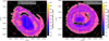 |
Fig. 12 Same as Fig. 11, but for a kappa distribution. |
| In the text | |
|
Fig. A.1 Examples of kappa electron flux distributions in the energy range [1 eV, 1 MeV] for different values of the κ parameter. These six kappa distributions have the same average energy of 50 keV and the same initial energy flux Q0 = 10mWm−2. The different κ parameters chosen for each distribution are displayed in the legend. |
| In the text | |
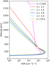 |
Fig. A.2 Profiles of the VER(z) modeled for each of the kappa distributions shown in Fig. A.1. |
| In the text | |
Current usage metrics show cumulative count of Article Views (full-text article views including HTML views, PDF and ePub downloads, according to the available data) and Abstracts Views on Vision4Press platform.
Data correspond to usage on the plateform after 2015. The current usage metrics is available 48-96 hours after online publication and is updated daily on week days.
Initial download of the metrics may take a while.