| Issue |
A&A
Volume 691, November 2024
|
|
|---|---|---|
| Article Number | A330 | |
| Number of page(s) | 19 | |
| Section | Galactic structure, stellar clusters and populations | |
| DOI | https://doi.org/10.1051/0004-6361/202451086 | |
| Published online | 25 November 2024 | |
Revisiting the local interstellar radiation field using Gaia DR3
INAF-Osservatorio Astrofisico di Arcetri,
L. E. Fermi 5,
50125
Firenze,
Italy
★ Corresponding author; simone.bianchi@inaf.it
Received:
12
June
2024
Accepted:
24
September
2024
Context. Dust grains in the interstellar medium are heated by the integrated radiation from stars in the Milky Way. Thus, knowledge of the local interstellar radiation field (LISRF) is necessary to interpret observations of dust emission in the infrared and constrain (some) properties of interstellar grains. The LISRF representation that is most widely used in dust modeling still dates back to the seminal works of Mezger et al. (1982, A&A, 105, 372) and Mathis et al. (1983, A&A, 128, 212).
Aims. A new version of the LISRF is presented here, starting from the photometry of the Gaia Data Release 3 (DR3) and revisiting the available data. This dataset includes observations from the Pioneer 10 and 11 probes.
Methods. The LISRF contribution by direct starlight was estimated in the Gaia bands by summing fluxes of all stars in DR3. The LISRF was extrapolated from the optical to the ultraviolet and near-infrared, using the astrophysical parameters provided by DR3 for a subsample of Gaia stars. The correlation between dust emission at 100 µm and residual diffuse emission in the Pioneer and other available maps was exploited to derive the contribution of dust-scattered starlight to the LISRF.
Results. The new LISRF is significantly redder and emits ~30% more energy than the old model. The old LISRF is almost a factor two lower in the near-infrared, while, in the optical, it accounts only for direct starlight. For |b| < 50°, diffuse starlight contributes on average to ~25% of the total radiation, which is three times more than what can be derived using literature estimates at high Galactic latitudes.
Conclusions. The new LISRF can modify the predicted mid-infrared (MIR) dust emission beyond the uncertainties normally assumed between dust models and observational constraints. These differences should be taken into account to redefine the properties of small grains and of carriers of the MIR emission bands.
Key words: dust, extinction / Galaxy: general / solar neighborhood / Galaxy: stellar content
© The Authors 2024
 Open Access article, published by EDP Sciences, under the terms of the Creative Commons Attribution License (https://creativecommons.org/licenses/by/4.0), which permits unrestricted use, distribution, and reproduction in any medium, provided the original work is properly cited.
This article is published in open access under the Subscribe to Open model. Subscribe to A&A to support open access publication.
1 Introduction
In the Milky Way (MW) and the majority of galaxies, stars emit most of radiation from the ultraviolet (UV) to the near-infrared (NIR). While light at wavelengths λ < 0.0912 µm is almost entirely suppressed after emission (through ionization of neutral hydrogen), at longer wavelengths, the diffuse interstellar medium (ISM) is generally exposed to the integrated radiation from all stars (nearby and distant) whose light has not been severely extinguished by interstellar dust. This interstellar radi-ation field (ISRF) is generally expressed as an average surface brightness or as a radiation energy density (the first definition is adopted here). The ISRF has a profound impact on the state of interstellar matter, as it regulates the energy states of atoms and molecules and ionizes them and the surface of dust grains, providing free electrons for heating the gas. In particular, the ISRF heats dust grains to temperature of a few tens of Kelvin, causing emission at mid- and far-infrared (MIR and FIR) and sub-millimeter (submm) wavelengths (for a general reference, see, e.g., Draine 2011).
While the ISRF is expected to vary within the MW, its direct measurement is only possible in the vicinity of the Sun. The so-called local ISRF (LISRF) can be derived from observations of the sky from the UV to the NIR. However, the estimate is complicated: when attempted from the ground, airglow and scat-tering from the upper atmosphere make up a substantial part of the foreground emission that needs to be taken into account; observations from near-Earth positions in outer space reduce (or remove altogether) it. However, another foreground source still needs to be considered, zodiacal light (sunlight scattered by interplanetary dust) and its thermal emission (for a review of these and other foregrounds, see Leinert et al. 1998). Finally large-area (ideally, whole-sky) observations are needed to avoid extrapolations and biases due to specific Galactic regions. Some of these issues were lifted in the late 70s/early 80s for UV space observations: those measurements, together with a few constraints in the optical from ground-based observations, were used by Mezger et al. (1982) to define a model of the LISRF. This was later updated by Mathis et al. (1983) to add a further constraint derived from (limited-area) NIR observations in the Galactic plane. In the following, I refer to the LISRF defined in these two works as the MMP model.
Since 1983, MMP became a popular representation of the LISRF and Mathis et al. (1983) was celebrated among other seminal papers in “The first 40 years” issue of this Journal (Jones 2009). The usage of the MMP formulation was later boosted by the launch of the Herschel (Pilbratt et al. 2010) and Planck (Planck Collaboration I 2011) satellites in 2009, which signifi-cantly increased the availability of MIR, FIR, and submm data, for the MW and other galaxies. In fact, starting from the origi-nal papers, the MMP has been mainly used as a tool to predict dust emission. For example, models for dust grains in the dif-fuse MW ISM are set to reproduce the dust emission at high Galactic latitude observed by satellites such as the InfraRed Astronomical Satellite (IRAS; Neugebauer et al. 1984), Cosmic Background Explorer (COBE; Boggess et al. 1992), and now Herschel and Planck, assuming that the heating field is the MMP LISRF (see, e.g., Désert et al. 1990; Dwek et al. 1997; Li & Draine 2001; Zubko et al. 2004; Compiègne et al. 2011; Siebenmorgen et al. 2014; Jones et al. 2017. Also, a (rescaled) MMP model is adopted when computing templates of dust emission under different heating intensities, used to interpret MIR-to-submm observations of galaxies (see, e.g., Draine et al. 2007; Galliano et al. 2011; Nersesian et al. 2019).
Only a limited number of new observational constraints has become available since the MMP papers. Most notably, the Dif-fuse Infrared Background Experiment (DIRBE) aboard COBE has mapped the NIR emission from the whole sky (Arendt et al. 1998); using LISRF estimates from these maps, Draine (2011) modified the MMP model, after seeing that its NIR output is lower than observations. On the contrary, Seon et al. (2011) found a lower UV LISRF than predicted by MMP, using a large sky area survey from the Science and Technology Satellite-1 (STSAT-1). In the optical range, instead, there has been no major update since the source-counts extrapolations and the ground-based estimates used by Mezger et al. (1982). The vast and complete catalogs of optical stellar fluxes from the Gaia satellite (Gaia Collaboration 2016) now offer the possibility to make a new estimate of the LISRF in the optical. Masana et al. (2021) used the photometry from Gaia Data Release 2 (DR2; Gaia Collaboration 2018) complemented with data from the HIPPARCOS satellite (Perryman et al. 1997), to derive the contribution of direct starlight to the radiation field; they further exploited a correlation between observed diffuse emission and 100 µm dust emission from IRAS to estimate the contribution of starlight scattered off dust grains in the ISM (from Kawara et al. 2017; see Sano & Matsuura 2017 for a review of other results in the liter-ature). However, Masana et al. (2021) have been interested in estimating the natural sky brightness at ground-based observing sites (including also zodiacal light, airglow, and radiative trans-fer through the atmosphere); they have not discussed the LISRF per se. Actually, an estimate on the LISRF in the optical, from a vantage point outside the interplanetary dust cloud and includ-ing both direct and scattered radiation, would have been possible using data from the Pioneer 10 and 11 probes (Weinberg et al. 1974). However, the data had been used to study diffuse MW emission (Gordon et al. 1998) as well as cosmic, extragalactic, emission (Matsuoka et al. 2011), but not the full LISRF.
The purpose of this work is to derive a new estimate of the LISRF starting from the Gaia Data Release 3 catalog (DR3; Gaia Collaboration 2023). First, in Sect. 2, I compute the optical LISRF from direct starlight in the Gaia photometric bands, using fluxes from Gaia (and HIPPARCOS for the brightest stars). In Sect. 3, I compare the results with MMP and other data, includ-ing, in particular, new optical estimates from the Pioneer probes (the full derivation of which is presented in Appendix A). In Sect. 4, I extrapolate the LISRF from the optical to the UV and NIR, using Gaia DR3-based parameters for stellar atmospheres; I also validate the results against full sky data (and against selected catalog cross-matches in Appendix B). The spectrum for diffuse radiation is derived in Sect. 5 using dust emission as a template. The full LISRF, including both direct and diffuse starlight, is presented and discussed in Sect. 6. As an application, in Sect. 7, I evaluate the impact that the new LISRF will have in the verification of MW dust models. My results are summarized in Sect. 8.
2 The LISRF in the Gaia photometric bands
Expressing the LISRF in terms of average surface brightness, it is
 (1)
(1)
where lλ is the surface brightness from a specific direction in the celestial sphere1. To show the contribution to Jλ of differ-ent parts of the sky, whole sky maps are presented in this work, adopting the Hierarchical Equal Area isoLatitude Pixelization (HEALPix2; Górski et al. 2005). Since all HEALPix pixels have the same area ΔΩ, Eq. (1) can be reduced to:
 (2)
(2)
where Npix is the total number of pixels in the map and  the surface brightness from each pixel. If one consider only direct starlight,
  , with
  the total flux from all the stars within the pixel. Equation (1) becomes
 (3)
(3)

showing that Jλ can be derived from a simple summation of the flux  of each star. In this work, HEALPix maps are used of order 6 (Npix = 49152, ΔΩ ≈ 2.5 × 10⁻⁴ sr ≈ 0.84 deg2).
In this section, I describe the derivation of Jλ in the three bands of the Gaia Photometric Instrument: G, GBP and GRP (λpivot = 0.62, 0.51, 0.78 µm, respectively; van Leeuwen et al. 2022), including all stars in Gaia DR3 and the bright stars in the catalog of the HIPPARCOS mission (ESA Pubblication divi-sion 1997), for which no Gaia photometry is available. Here and in the rest of the paper, Iλ and Jλ will be expressed in units of W m−3 sr−1 (equivalent to 10−3 erg cm−2 s−1 µm−1 sr−1). In these units, Iλ and Jλ in the optical range have values of order unity.
2.1 Gaia
The DR3 contains photometric information for about 1.8 billion objects in G, and for about 1.5 billion in GBP and GRP (Gaia Collaboration 2023). In order to construct the map of Iλ, I extracted from the main source catalog3 (gaia_source) the source_id field, which encodes the position in the HEALPix representation; and the phot_g_mean_flux, phot_bp_mean_flux, phot_rp_mean_flux fields, containing the stellar flux in the three bands. The native fluxes were con-verted to units of energy per unit time, surface, and wavelength using the conversion factors provided in Sect. 5.4.1 of the DR3 documentation (van Leeuwen et al. 2022).
The fluxes of bright stars were corrected for saturation effects, using the magnitude-dependent formulas in Riello et al. (2021). These corrections account for minimal variations in the final Jλ values: only 0.2% in G, and about 1% in GBP and GRP. For simplicity, I did not consider the ~5 million stars with missing G photometry in the main photometric catalog, for which alternative estimates are given in a supplementary catalog (Riello et al. 2021); they would only account for variations in Jλ of about 0.01% in G, and about 0.1% in GBP and GRP. Instead, I applied corrections for the ~0.5 billion stars without GBP and/or GRP fluxes, following a procedure similar to what done by Masana et al. (2021): I first derived the average GBP/G and GRP/G ratios within each pixel – using stars with the complete photometric dataset; then, I assigned a flux according to the G value and the corresponding flux ratio. Nevertheless, these objects contribute to only 0.7 and 1.2% of Jλ in GBP and GRP.
In Fig. 1, I show the contribution of stars of different magnitude to Jλ, for the three Gaia photometric bands. The maximum contribution to Jλ, in all bands, comes from stars with magnitudes ≈10. For magnitudes ≲2, the distributions shows a break (most evident for G) due to the lack of very bright stars in the Gaia catalog: I will try to recover these using the HIPPARCOS catalog (Sect. 2.2). On the faint-end side, the distributions drops smoothly: in G, it goes down to the DR3 completeness limit at ≈ 21 magnitudes (Gaia Collaboration 2021). Masana et al. (2021) estimated the ratio between the total flux of fainter stars with G > 21 and brighter stars with 10.5 < G < 20, as a function of the position in the Galaxy: judging from their Fig. 4, the contribution of fainter stars is, at most, 5% for lines of sight in the inner disk (for Galactic longitudes |b| ≤ 90° and latitudes |l| ≤ 10°) and 0.05% elsewhere. Using these value and a full sky map for objects with 10.5 < G < 20, I find that faint stars can contribute a maximum of 1% to Jλ in the G band; this value is similar to the contribution of the last populated bin in Fig. 1. In principle, this value should be added to the calculation to derive an upper value for Jλ in the G band. However, given the negligi-ble extent of this contribution and its gross estimate, I preferred to avoid a cumbersome notation and consider it instead as an uncertainty in the estimate of Jλ, with the caveat that the value presented here is biased low with respect to the full Jλ including stars with G > 21, but still compatible within 1%. Since the Jλ distributions for GBP and GRP are very similar to that for G, I used the same uncertainty also for those bands.
A small fraction of the LISRF is due to extragalactic objects. Estimates based on galaxy counts predict Jλ ≈ 0.01 W m−3 sr−1 over the bands considered here (Driver et al. 2016). If the poten-tial contribution of distant galaxies to DR3 is selected, using the fields in_galaxy_candidates, in_qso_candidates and in_andromeda_survey, similar values are found: Jλ = 0.008, 0.01 and 0.007 W m−3 sr−1, for G, GBP, and GRP respec-tively. However, there is no guarantee on the completeness and purity of the DR3 extragalactic selections; for example, the Gaia Andromeda Photometric Survey (Evans et al. 2023) selects all objects (including Galactic stars) within 5.5° of M31; also, I found an anomalous concentration of objects near the Galac-tic center, namely, Galactic stars misclassified as extragalactic objects. Therefore, the values above are likely upper limits to the true extragalactic contribution from DR3. In this work, I have retained the Gaia “extragalactic” contribution in our estimates, noting that it might contain a dominant fraction of stellar radi-ation and extragalactic fluxes (albeit underestimated) should be added to the local radiation field. On the other hand, adding the estimates from independent galaxy counts will result in an upper limit to the total Jλ, since a fraction of extragalactic objects are indeed present in the Gaia catalog. Thus, analogously to what has been done for faint stars, in this work, I have considered the value from galaxy counts as a further uncertainty on the total Jλ.
The surface brightness map computed from Gaia is shown in Fig. 2, for the G band; its average, the LISRF Jλ, is presented in Table 1, for the three Gaia bands. The uncertainty results from the sum, in quadrature, of the uncertainties on the contribution of very faint stars and extragalactic objects, discussed above; and of a further 1% uncertainty in the photometric absolute calibration (van Leeuwen et al. 2022). Instead, the total contribu-tion of the photometric errors listed in the catalog is irrelevant, being an order of magnitude smaller than the other components I considered here.
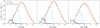 |
Fig. 1 Jλ vs. Gaia magnitudes, for stars in the Gaia and HIPPARCOS catalogs, and for HIPPARCOS stars with no Gaia counterpart. |
2.2 HIPPARCOS
Very bright stars are not included in the Gaia catalog, because of saturation. I recovered the contribution to Jλ of those objects using the HIPPARCOS catalog. First, the photometry in the Gaia bands is derived for the ~118 000 HIPPARCOS stars: I used the catalog HP photometry and V-I colors and the Riello et al. (2021) transformations, after verifying that V-I values are in the range of applicability of the formulas (for about 1200 stars with missing V-I, I used the mean value in the corresponding parts of the sky).
The Jλ values for the whole HIPPARCOS catalog are about one third of the Gaia values (Table 1). A substantial part of these Jλ must be due to stars already included in the previous estimate. According to the DR3 cross-match between the two catalogs, available from the Archive, ~85% of the HIPPARCOS stars has “best-neighbor” Gaia counterparts. The values of Jλ for this subsample are ~65% of the full HIPPARCOS estimates; those derived from the HIPPARCOS photometry are within ≲2% of the corresponding values obtained directly from Gaia photometry, providing an indication on the uncertainties on the photometric transformations used here (Table 1; see also Appendix B.3).
In principle, it would be possible to isolate the contribu-tion of stars missing from the Gaia catalog by selecting the HIPPARCOS stars not included in the cross-matching. This is the approach taken by Masana et al. (2021). Using DR2, they concluded that these stars account for ~20% of the total stellar radiation in G. However, Marrese et al. (2019) argued that only a small fraction of HIPPARCOS stars should be really out of the Gaia catalog and that the majority of the missing counter-parts in the cross-match is due to problems with the astrometric solutions. For an independent check on the overlap between HIPPARCOS and Gaia, I also plot in Fig. 1 Jλ for HIPPARCOS. If the bright and faint end sides are excluded and only the range 3 < G < 6 is considered, the Jλ distributions for Gaia and HIPPARCOS are essentially the same, meaning that the same stars are present in both. While the drop in Jλ for G ≳ 7 is expected due to the shallower completeness limit of HIPPARCOS, the val-ues of Jλ for G ≲ 2 are almost entirely due to HIPPARCOS stars missing from Gaia.
Beside the official best-neighbor cross-match, Marrese et al. (2019) provide the results of a nearest-neighbor cone search of HIPPARCOS stars within 1″ of a Gaia star. About 1500 HIPPARCOS stars are missing from this alternative list (com-pared to the 19 000 missing from the DR3 cross-match). Here, I assume that these stars are the ones that are truly missing from DR3 and whose photometry is only available from the HIPPAR-COS catalog; indeed, their Jλ versus magnitude distribution is complementary to that of Gaia (Fig. 1).
The surface brightness map resulting from the independent HIPPARCOS contribution is shown in Fig. 2, for the G band; the Jλ values for all bands are presented in Table 1. The uncertainty on Jλ was estimated by applying simple magnitude cuts to the HIPPARCOS catalog in correspondence to the bright-end drop of the Gaia distribution shown in Fig. 1. It is about 15% of the HIPPARCOS final contribution, reflecting the uncertainty in the choice of the contributing stars (larger than the uncertainty in the photometric transformations discussed above). As made evident by the very sparsely populated map in Fig. 2, the HIPPARCOS-only contribution is dominated by a small number of nearby bright stars. For example, there are only 68 objects with G < 2, constituting almost 90% of the value of Jλ for the G band listed in Table 1. The final LISRF from direct starlight, resulting from the combination of the Gaia and HIPPARCOS catalogs, is also given in Table 1.
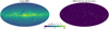 |
Fig. 2 G-band surface brightness, IG, from the Gaia DR3 catalog (left) and from the HIPPARCOS stars not in DR3 (right). To ease the visualization of the HIPPARCOS contribution, both maps are been smoothed with a Gaussian of FWHM equal to the pixel size. All maps in this work are shown in Galactic coordinates and Mollweide projection (the extent of each map being delimited by Galactic latitude b = −90° at bottom and b = 90° at top, and by Galactic longitude l = −180° at right and l = 180° at left, respectively). |
Contribution of direct starlight to the LISRF in Gaia bands, plus estimates for other samples.
3 Comparison with MMP and full-sky surveys
The Jλ values estimated in the previous section are compared with the MMP LISRF model in Fig. 3. In the optical-NIR range, the MMP model consists of the sum of three “dilute” (i.e., scaled-down) blackbodies. In its original derivation (Mezger et al. 1982) the blackbodies were just two: the dilution factors were chosen to broadly reproduce near-UV estimates from satel-lite and B-band estimates from ground-based observations (from Lillie 1968, as reported by Witt & Johnson 1973), along with B and V-band estimates from stellar counts (as tabulated in Allen 1973). Mathis et al. (1983) made a few modifications and intro-duced a third dilute blackbody to match estimates of the LISRF in the NIR, extrapolated from rocket-borne observations in the Galactic plane at 2.4 µm (Hayakawa et al. 1978). Nevertheless, the values of Jλ in the optical range changed little with respect to Mezger et al. (1982). The MMP model is shown in Fig. 3, together with the observational data from which it has been derived. The model is very close to our estimates and when I used it to derive synthetic photometry in the three Gaia bands, I found a difference within ≲4%; this is much lower than the 15% uncertainty claimed by the authors. Thus, at least in the opti-cal range, MMP is a good representation of the direct starlight component of the LISRF.
The NIR component introduced by Mathis et al. (1983) proved insufficient to explain the LISRF resulting from full-sky DIRBE observations (Arendt et al. 1998). To match the newer NIR data, Draine (2011) used the two dilute blackbodies of Mezger et al. (1982) and increased the dilution factor of the third blackbody of Mathis et al. (1983). To my knowledge, the DIRBE values are only shown graphically in Fig. 12.1 of Draine (2011) and are not provided numerically elsewhere. I estimated them directly from the maps (see Appendix A.1 for the deriva-tion). The Draine (2011) LISRF and the DIRBE estimates are also shown in Fig. 3. Beside roughly matching the DIRBE dat-apoints, the new LISRF model is significantly brighter in the optical; when integrated over the G band, Jλ is ~40% higher than the corresponding Gaia/HIPPARCOS value (note: the synthetic Gaia photometry for Draine 2011 is not shown in the figure).
Both MMP and the Draine (2011) LISRF share the same spectrum for λ ≲ 0.25 µm. Below the hydrogen ionization thresh-old, the spectrum is described as a broken power law which Mezger et al. (1982) scaled on a few Jλ estimates: in the far-UV, using data for about 1/3 of the sky (but extrapolated to the whole celestial sphere) taken with a spectrometer on board the Apollo 17 spacecraft (Henry et al. 1980); for 0.15 ≲ λ/µm ≲ 0.3, from a full-sky survey from the TD-1 satellite (Gondhalekar et al. 1980); for 0.2 ≲ λ/µm ≲ 0.5, from observa-tions of selected areas from the OAO-2 satellite (plus additional optical ground-based observations; Lillie 1968). The UV Jλ values are shown in Fig. 3, where I adopted as the errors the cal-ibration uncertainty quoted by Henry et al. (1975) for the far-UV spectrometer, the total uncertainty (dominated by calibration) quoted by Gondhalekar et al. (1980) for the TD-1 estimates, and the spread in the determinations of Lillie (1968) shown by Witt & Johnson (1973). In a more recent work, Seon et al. (2011) derived Jλ using far-UV data for about 80% of the sky, from the Far-Ultraviolet Imaging Spectrograph (FIMS) on the STSAT-1 satellite: their values are lower than previous estimates (see Fig. 3, where I plot the extremes of a rather featureless spec-trum), but still marginally compatible within the large calibration error of the instrument (Edelstein et al. 2006). Some of the UV and NIR observational constraints will be also used from the next section, where the Jλ spectrum is extrapolated beyond the Gaia bands.
An advantage for the measurement of the sky radiation field was that of the Pioneer 10 and 11 probes. The Imaging Pho-topolarimeters (IPPs) aboard these spacecrafts have made several measurements, covering ≈90% of the sky, in two photometric bands in the optical range. In their cruise to outer space, the two probes went beyond the interplanetary dust cloud, thus avoid-ing one of the sources of uncertainties in the estimate of the LISRF from near-Earth positions: zodiacal light. The Pioneer 10/11 data have been used to study the diffuse galactic and extra-galactic light (Toller et al. 1987; Toller 1990; Gordon et al. 1998; Matsuoka et al. 2011). The data has been distributed after removing the fluxes of bright stars (V < 6.5). Thus, in order to recover the full LISRF, this contribution has to be added back; this is done in Appendix A.2. The total Pioneer estimates are shown in Fig. 3; they include both direct starlight and diffuse light scat-tered by dust in the ISM (diffuse starlight is also included in the UV and NIR full-sky estimates discussed above). The Pioneer-based Jλ values are higher (by ~40% in G) than the starlight-only estimates from Gaia/HIPPARCOS (or MMP), highlighting the necessity of including diffuse radiation in the LISRF evaluation. This is described in Sect. 5.
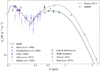 |
Fig. 3 Comparison between the Gaia/HIPPARCOS estimates and MMP. Also shown: the observational constraints of MMP (listed in the bottom-left legend); synthetic photometry of the MMP model over the Gaia bands; the Draine (2011) update based on DIRBE full sky data; our estimates from Pioneer 10/11 data; and the more recent UV estimates from Seon et al. (2011). See main text and Appendix A for details. |
4 The LISRF spectrum for direct starlight
In this section, I use models of the spectra of Gaia and HIPPAR-COS stars to extrapolate Jλ beyond the Gaia bands. For each star, the observed (i.e., dust-attenuated) spectrum fλ can in principle be derived from the observed flux in the G band if we have a good model of the intrinsic, unattenuated, spectrum  and the reddening is known. Assuming for the moment that observations are done at a specific wavelength (e.g., the central wavelength of the G band) and not integrated over a filter bandwidth, we can write:
 (5)
(5)
where fG is the flux at the central wavelength of band G and  is the flux that would be observed in the absence of dust extinc-tion. The dust extinction, Aλ, can be written as the product of A0, the extinction at a reference wavelength, and Eλ, the extinc-tion law normalized at the same wavelength; analogously, AG is the dust extinction at the central wavelength of band G. In prac-tice, Eq. (5) is the result of three passages: first, the observed fG is dereddened for extinction AG to obtain the intrinsic flux; second, the full intrinsic spectrum is recovered by scaling the flux model
  to the intrinsic G flux; and, finally, the full observable spectrum can be obtained by correcting the unreddened spectrum for the reddening Aλ, at each λ.
Equation (5) can be easily generalized to the case of a broad filter by defining
 (6)
(6)
where the integration is over the filter band and Sλ is the filter response function; and
 (7)
(7)
For very narrow Sλ (like, e.g., a delta function), AG tends toward the extinction at the filter central wavelength. For a broad filter, such as the Gaia G band, AG will instead be higher for intrinsically bluer stars and lower for redder ones.
In the following, I describe how I used Eq. (5) to derive fλ values for each star in a catalog and summed their individ-ual contribution to obtain Iλ maps and Jλ. For  , I used the library of stellar atmospheres of Castelli & Kurucz (2003); for Eλ, the average (RV = 3.1) MW extinction law of Fitzpatrick (1999). The spectrum was sampled (and averaged) over a grid of 99 wavelength bins, logarithmically spaced between 0.1 and 4.3 µm.
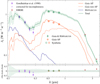 |
Fig. 4 Direct starlight component of the LISRF spectrum. Upper panel: Total spectrum, the spectrum of Gaia AP stars, the recovered spectrum of Gaia non-AP stars, and the spectrum of the HIPPARCOS stars not included in the Gaia catalog. For the total spectrum (and for the Gaia AP com-ponent) I also plot the synthetic Jλ values in the Gaia bands together with the esti-mates from the direct flux summation. I also show observational UV and NIR estimates and the corresponding synthetic photome-try (for the full spectrum only). The relative difference between observations and syn-thetic photometry is shown in the bottom panel. The shaded area refers to the esti-mated uncertainty for the total spectrum (see text for details). |
4.1 Gaia
The DR3 provides astrophysical parameters (APs) for about 470 million stars, derived by fitting BP and RP low resolution spectra with an extended library of various synthetic stellar atmosphere models (for details, see Andrae et al. 2023; Creevey et al. 2023). I use here a subset of AP quantities, obtained from the best-fitting spectral library and available in the main gaia_source catalog.
I derived the unattenuated stellar spectrum,  , from the effective temperature Teff (teff_gspphot), the surface gravity log ɡ (logg_gspphot), and the metallicity [M/H] (mh_gspphot). About 90% of the fitted parameters are within the grid boundaries of the Castelli & Kurucz (2003) library adopted here (the original libraries used for the APs derivation are not publicly available); for the rest, I assumed the values at the nearest boundary. In practice, I pre-computed spectra over a table spanning 100 logarithmically spaced temperature val-ues within 2400 K< Teff <42 000 K; 25 log ɡ values within −0.5 < log ɡ < 5.5; 45 [M/H] values within −4.5 < [M/H] < 1 (those are the boundaries of the AP estimates). When deriving the spectrum for each star, I simply searched for the nearest entry in the table: for the adopted grid, there is virtually no difference between this and a table interpolation.
The dust-extinguished spectrum is derived according to Eq. (5), using the monochromatic extinction A0 at 0.5477 µm (azero_gspphot), the G-band extinction AG (ag_gspphot), and the average Fitzpatrick (1999) extinction law (also used for AP estimates). While the results shown here use the AG from APs, there is little difference if the same quantity is derived from Eq. (7) computed over our spectrum grid (plus an additional grid in A0).
In Fig. 4, I show the final spectrum resulting from Gaia stars with available APs. I also include Jλ derived from the direct sum-mation of the fluxes of AP stars in the three Gaia bands (values are presented in Table 1), along with the synthetic photometry obtained by integrating the spectrum over the filter bandpasses. While the agreement in the G band is almost by construction, the closeness between the GBP and GRP values and the synthetic photometry was not granted, given the differences between the AP stellar libraries and the one adopted here.
The intensity and color ratios of the photometric Jλ for the AP selection are clearly different from those of the full stellar derivation of the previous section (also shown in Fig. 4) or from the values for Gaia stars only (from Table 1). This is due to the complex selection applied to the full Gaia sample before producing the AP catalog. First, the fit was not attempted for stars with G > 19, amounting to 2/3 of Gaia entries. The fits on the remaining objects were further filtered before publishing the catalog, leaving out about 100 thousand stars, preferentially of brighter G and lower signal-to-noise in the parallax deter-mination (Andrae et al. 2023). In Fig. 5 we show the separate contribution of AP and non-AP stars to JG, as a function of the G magnitude and of the GBP − GRP color. The distribution with magnitude (top panel) shows that AP stars contributing most to JG are on average fainter than non-AP stars, lacking in partic-ular the very-bright stars: this is the reason of the reduced Jλ values. Instead, the omission of G > 19 stars has, as expected, little impact on the total values. The distribution with colors of all Gaia stars (bottom panel) shows two main peaks: stars with the largest contribution to JG have GBP − GRP ≈ 1.2, followed by those with GBP − GRP ≈ 0.8. In the AP selection, the red-der peak is preferentially suppressed with respect to the bluer one, probably as a result of the selection against poorer paral-lax measurements, leaving out redder, more distant stars. The net effect is that the photometric Jλ values for AP stars (and the corresponding spectrum) are bluer than for the full catalog.
The final step is to recover the spectrum of Gaia stars with-out APs. I adopted a simple procedure for this purpose: i) using the binning in GBP − GRP shown in Fig. 5, I derived the aver-age spectrum from all AP stars in each color bin and each pixel, and normalize it to the corresponding JG value; in case there were no AP stars in a particular bin for a given pixel, I used the whole-sky average for that color bin; ii) I assumed that the same spectral shape is valid on average for the contribution of non-AP stars in the same color bin and pixel; and iii) I scaled the average spectrum by the JG contribution of non-AP stars. The resulting spectrum is shown in Fig. 4. As expected, it is redder than the Jλ from AP stars.
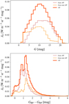 |
Fig. 5 JG vs. G (top) and vs. GBP – GRP (bottom), for Gaia stars with and without APs. |
4.2 HIPPARCOS
For HIPPARCOS stars, I followed Seon et al. (2011) and derived Teff and log g from spectral types, using the tables of Straizys & Kuriliene (1981); in this case I assumed solar metallicity. The spectral types are taken from the HIPPARCOS catalog and sup-plemented with data from the SIMBAD database4, after clearing peculiar entries. Whenever available from SIMBAD, direct Teff and log ɡ estimates are preferred; at the time I accessed the service (May 2023), they did not include Gaia AP values and are thus independent. The full spectral classification (either from spectral types or direct estimates) is available for ~65% of the catalog. For an additional ~34% the spectral type is not complete, missing (in the vast majority of cases) the luminosity class of the star: in this case I draw it randomly from the sample with the full description. The rest of the objects (1%) are assumed to be stars of solar spectral type (G0V). The final result of this procedure is the association of each HIPPARCOS star to its respective entry in a table of ~ 190 spectra, again derived from the Castelli & Kurucz (2003) library over the adopted wavelength grid.
The monochromatic extinction A0 is derived by comparing observed stellar colors and the intrinsic spectra assigned to a star. In practice, I used the spectrum to compute synthetic colors as a function of extinction; then I select the A0 value for which the synthetic color matches the observed one. For each star, I derive up to six A0 values, using as colors B − V, V −I, BT − VT, HP − I, V − J, I − K (B, V, I, BT, VT, and HP from the HIPPARCOS catalog, J and K from SIMBAD, the full set being available for 95% of HIPPARCOS stars). I used as A0 the average of these estimates. For each spectrum and A0, AG is derived using Eq. (7). Finally, the spectrum fλ is computed for each star using Eq. (5) and the fG value derived in Sect. 2.2. The Jλ spectrum for the HIPPARCOS stars not included in the Gaia catalog is shown in Fig. 4 (note: other spectra from different subsets of the catalog are presented in Appendix B).
4.3 Results
Several pitfalls can affect the extrapolation of stellar spectra dis-cussed in the previous sections: the APs are derived from optical data only and might be affected by the extinction-temperature degeneracy (Andrae et al. 2023); the spectral libraries used for the AP fitting are not the same as the Castelli & Kurucz (2003) library I use here. In particular, the average MW extinction law might not be adequate along all sight-lines, in particular in the UV. The caveats on the extinction law and on the extinction-temperature degeneracy apply both to the Gaia and HIPPARCOS derivation; for the latter, there is also the additional issue that the stellar parameters and extinctions come from heterogeneous sources and thus have not been derived simultaneously and self-consistently. Despite all these (and possibly other) sources of uncertainties, I find that the extrapolated spectra are still reliable, at least for Jλ resulting from the contribution of a large number of stars. The verification of the method is presented in Appendix B: in short, I have selected various cross-matches between indepen-dent photometric catalogs and the Gaia/HIPPARCOS ones and compared Jλ derived from UV, optical, and NIR photometry with synthetic photometry in the same bands, from the extrap-olated spectra. Here, I assume as relative error for the total Gaia spectrum (AP stars plus non-AP extrapolation) the relative error found for the samples analyzed in Appendix B, along with the corresponding one for HIPPARCOS. The final uncertainty is the sum in quadrature of both contributions.
The total Jλ from direct starlight is shown in Fig. 4, together with its uncertainty. Synthetic photometry in the Gaia bands compares well with the direct summation of Gaia and HIP-PARCOS fluxes, but not as well as for Gaia AP stars only: the difference in G is still within the error quoted in Table 1, but about twice in the GBP and GRP bands. The reason of the larger uncertainty is in the gross estimate of the spectrum of Gaia stars without APs. Nevertheless, the difference is well within the con-servative estimate of the global Jλ uncertainty, which is about 7% in the optical and NIR.
An estimate of Jλ in the UV is obtained by Gondhalekar (1990) by summing the fluxes from stars observed by the TD-1 satellite. He used a revised version of the original catalog by Thompson et al. (1978), with recalibrated fluxes resulting in a calibration uncertainty of 10% (about half of that quoted for the full − direct + diffuse starlight – estimate of Gondhalekar et al. 1980). Synthetic photometry from the spectrum is in good agreement with the estimate from the TD-1 catalog, except at 0.274 µm. However, that flux in particular might be affected by incompleteness in the catalog. If I correct the Gondhalekar (1990) Jλ for the incompleteness factors estimated in that work, all UV values agrees with the starlight spectrum within their errors, and within the current estimated uncertainty, ~13% in the UV. Apparently, Gaia & HIPPARCOS stars account for all the UV starlight emission. In particular, the limited number of very bright and nearby stars present only in the HIPPARCOS catalog contribute to almost half of Jλ in this range. The important contribution of nearby stars is also evident in the simulated Iλ map at 0.15 µm (i.e., the GALEX FUV band, one of the TD-1 bands, or the L-band in Seon et al. 2011), shown in Fig. 6. Despite lacking a contribution from diffuse starlight, the map shows sim-ilar features as those detected in far-UV surveys (Henry et al. 1977; Gondhalekar et al. 1980; Seon et al. 2011), namely: an asymmetry in Galactic longitude along the disk, between the 0° < l < 180° and the brighter −180° < l < 0° ranges; the distri-bution of OB stars in the Gould Belt, inclined with respect to the Galactic plane and particularly evident in the second longitude range (compare the map with the sky distributions of Gould Belt stars from de Zeeuw et al. 1999, as shown by Hohle et al. 2008). The same features are visible also in optical Iλ maps derived from the HIPPARCOS catalog (e.g., the V < 6.5 direct starlight map in Fig. A.2), confirming the local origin of most of the LISRF in the UV.
In the NIR, the DIRBE Jλ values can be used as estimates of the LISRF from direct starlight, if observations are excluded at 1.25 µm, where the contribution from dust-scattered radiation might be significant (see next section). In Fig. 6 I show the predicted Iλ map in the DIRBE 2.2 µm band. The Iλ dis-tribution on the plane in front of the Galactic bulge shows a depression (correspondent to the optical extinction lane) which is not as evident in the map from observations, at least at the DIRBE resolution (Fig. A.1). The difference is also shown by the Galactic longitude (for |l| < 45°) and latitude (at b ≈ 0°) profiles of Fig. 7; it can be explained by the presence, in the central part of the disk, of stars heavily extinguished in the opti-cal and with emission peaking in the NIR, which are missing from the Gaia catalog (and thus from the current predictions; see also Hobbs et al. 2021). Despite this, the missed population does not seem to contribute significantly to Jλ: the difference between the current estimate and observation at 2.2 µm is of the same order of the adopted NIR uncertainty (Fig. 4). The agreement also shows that the modeling of the spectrum of non-AP stars is not substantially incorrect. At 3.5 µm, instead, the observed Jλ is 13% higher than the prediction, almost twice the refer-ence uncertainty. This could be attributed in part to the missing population described above and the uncertainties in the model-ing; and in part to dust emission, which starts to be significant at this wavelength (Arendt et al. 1998), mainly because of the 3.2 µm feature of Polycyclic Aromatic Hydrocarbons (Draine 2011). Sano et al. (2016) studied the various contributions to the emission detected by DIRBE and found that diffuse Galactic light at 3.5 µm accounts for about 5% of total starlight, a correc-tion that would make the Jλ estimate marginally consistent with the adopted uncertainty. However, their result was obtained for high Galactic latitude only, where the uncertainties due to the contribution of zodiacal light in emission are high. Therefore, I no dot apply this correction and simply take note of this differ-ence. Overall, the Jλ spectrum for direct starlight shown in Fig. 4 reproduces the (few) observational constraints rather well.
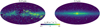 |
Fig. 6 Predicted Iλ from direct starlight at 0.15 µm and 2.2 µm. Maps have been smoothed with a Gaussian of FWHM=0.7° to match the resolution of DIRBE (and approximately that of the map in Seon et al. 2011). |
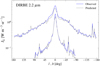 |
Fig. 7 Profiles in the DIRBE 2.2 µm band, along Galactic longitude l (averaged for |b| < 15°) and Galactic latitude b (averaged over the whole l range). |
5 The LISRF spectrum for diffuse radiation
Diffuse Galactic radiation scattered by dust has received more attention than the total LISRF, because it allows us to study the dust scattering properties and to access the lower layer of emission, namely, the extragalactic background light. Isolating its contribution suffers from the same problems as the full LISRF study, namely: terrestrial airglow and zodiacal light, plus the additional burden of subtracting direct starlight (either via cat-alogs, removal of point sources, or selection of blank sky areas). A way to overcome these issues is to study the fraction of radia-tion that spatially correlates with an independent tracer of dust, such as emission in the FIR (Brandt & Draine 2012). Correlations between diffuse radiation and emission at 100 µm observed by the IRAS satellite, Iν(100 µm), have been studied from the UV to the NIR by several authors (Murthy et al. 2010; Arai et al. 2015; Kawara et al. 2017; Chellew et al. 2022).
In a first attempt to model the diffuse radiation, I followed Masana et al. (2021) and exploited the published correlations to derive maps of  from those of Iv(100 µm). From
  , the diffuse component of the LISRF Jλ is then computed. I verified the validity of the
  maps by comparison with maps of dif-fuse emission that can be derived from the observations and the direct starlight estimates of the current work. For each of the two Pioneer and the DIRBE 1.25 µm bands, I used the map presented in Appendix A (including all emission components) from which I subtracted a map of direct starlight, estimated by integrating the spectra of Sect. 4 over the filter bandpasses and convolving the result by the appropriate resolution: I used FWHM = 4° for the Pioneer data, with an area close to the average field-of-view of the IPP instruments; and 0.7° for DIRBE. For the NUV and FUV bands, I directly used the background maps derived by Murthy (2014) from observations taken by GALEX: they were obtained after masking point sources and averaging over various fields, and cover most of the sky, but excluding the galactic plane. From each of the maps described above, I further subtracted the value of the extragalactic background listed in Driver et al. (2016); however, this does not modify significantly the results. I note here that the contribution of zodiacal light is absent in the Pio-neer bands, while was removed using a model from DIRBE and GALEX maps. In Fig. 8 I show the maps of
  for the BIPP, FUV and 1.25 µm bands, and in Fig. 9 the surface brightness profiles along Galactic latitude, averaged over the whole longitude range, for all the five bands I considered. Figure 9 also presents the profile for Iν(100 µm) from the map of Schlegel et al. (1998), after subtracting a cosmic background of 0.34 MJy sr−1 (Driver et al. 2016).
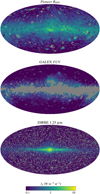 |
Fig. 8 Maps of |

5.1 The “literature” solution
Brandt & Draine (2012) study residual emission at high galactic latitude in 92000 blank-sky optical spectra from the Sloan Digi-tal Sky Survey (SDSS). The works has been recently revised by Chellew et al. (2022), by expanding the sample of SDSS blank-sky spectra to ~250000, and including dust self-absorption. They use the 100 µm maps from the IRIS reprocessing of IRAS data (Miville-Deschênes & Lagache 2005). Assuming that dust emission is due to radiation absorbed from the LISRF, Iv(100 µm) scales as the product of the LISRF intensity and the dust column density. In the case of low dust column density, Iv(100 µm) should correlate linearly with any emission from scattered starlight. As the dust optical depth increases, however, only a fraction of the column density contributes to scattering starlight in the direction of the observer. This effect is taken into account by Chellew et al. (2022) by assuming
 (8)
(8)

where the correction factor, βλ, depends on the optical depth, τλ, for the diffuse radiation: in the optically thin case,  is proportional to Iv(100 µm), while in the optically thick case it saturates to a value independent of the line of sight (both τλ and Iv(100 µm) being dependent linearly on the dust column density). The authors derived τλ from the Schlegel et al. (1998) extinction maps, assuming the average extinction law of Fitzpatrick (1999).
Using the same data and the results from Chellew et al. (2022), I derived a map for  from the IRIS map Iv(100 µm), over the wavelength range analyzed by the authors (0.4 ≲ λ/ µm ≲ 0.9) and the entire sky. The analyses of Brandt & Draine (2012) and Chellew et al. (2022) suffer from a bias of uncertain origin, which can be corrected by a multiplicative factor. I also scaled the
  maps for this factor, and derive Jλ. This is shown in Fig. 10, together with the larger source of uncertainty estimated by the authors, namely, that on the bias factor itself. I label this and other estimates directly based on published correlations as the “literature” solution. There are clearly other uncertainties that are difficult to estimate, since I applied to the entire sky the results of Chellew et al. (2022), which are based on data at high Galactic latitude and mainly around the Galactic North Pole. In particular, I estimated
  also on the Galactic plane, where the emission traced by Iv(100µm) in specific regions might not be directly related to the dust column density, because of dust heating by localized star-forming regions and not by the average LISRF.
Kawara et al. (2017) adopted a similar approach to Brandt & Draine (2012) and fit emission in blank-sky spectra from the FOS instrument aboard the Hubble Space Telescope (HST), with a model that included diffuse starlight and zodiacal light. Diffuse starlight is modeled using the Iv(100 µm) map from Schlegel et al. (1998), after subtracting an extragalactic background of 0.8 MJy sr−1. The sky coverage is smaller than in Brandt & Draine (2012) and Chellew et al. (2022), being limited to just 54 pointings, but it includes data at low Galactic latitude. The model includes a linear dependence of  on Iv(100 µm), for the optically thin regime, and a negative term depending on the square of Iv(100µm), to take into account the saturation at high optical depths (see also Ienaka et al. 2013). I derive lλ and Jλ from the data and analysis of Kawara et al. (2017) for 0.2 ≲ 2/µm ≲ 0.7. Since the formulation chosen by Kawara et al. (2017) cannot be applied beyond the Iv(100µm) range they studied (otherwise the quadratic term prevails and the diffuse emission becomes negative), I assume that the correlation saturates for Iv(100 µm)≥ 50 MJy sr−1 (corresponding to a visual extinction of ~5; Ienaka et al. 2013; Chellew et al. 2022). The corresponding Jλ in shown in Fig. 10, together with the errors from the correlation estimated by the authors.
Arai et al. (2015) studied the diffuse radiation in NIR spectra taken in a few moderate-to-high Galactic latitude fields, by using the LRS instrument aboard the sounding-rocket borne Cosmic Infrared Background Experiment (CIBER). They assumed a simple linear relation between diffuse starlight and Iv(100 µm) (from Schlegel et al. 1998); this is because, in their fields and at the wavelength they explored (0.95 ≤ λ/µm < 1.65), the opacity is small. They also included zodiacal light in the modeling. As for the previous works, I used their results, while assuming that the ratio between scattered light and FIR radiation saturates for Iv(100 µm)> 50 MJy sr−1 (where extinction becomes ≥ 1). Thus, I was able to mimic the change from the optically thin to the optically thick regime (Fig. 10).
The same approach was adopted when deriving Jλ in the UV (Fig. 10). I used the linear correlation found by Murthy et al. (2010) from the background FUV and NUV GALEX maps already discussed above. In this case, I imposed saturation at Iv(100 µm) ≥ 10 MJy sr−1, when the medium becomes optically thick in the GALEX bands (Murthy et al. 2010).
The wide span of methods, sky coverage, and dynamical ranges used in the works described in this section reflects the piece-wise aspect of the spectrum (shown in Fig. 10). To obtain a unique “literature” solution over the whole UV-to-NIR wavelength range, I (rather arbitrarily) constructed an interpolated Jλ spectrum passing between the various estimates. Beyond the wavelength ranges studied in the literature, I assumed that the spectrum of diffuse light is constant for λ ≤ 0.15 µm, and goes to zero for λ > 2 µm. The spectra derived from the various works are within 25% of the interpolated solution. Finally, I produced  maps from the various results and scaled them to match the interpolated spectrum.
In Fig. 9 I plot the Galactic latitude profiles of the  maps from the “literature” solution, for the bands at which I derived observation-based estimates. Apparently, the “literature” solution is not able to match the observations in the optical and NIR. Instead, the agreement between model and observations is good in the FUV (right panel) and also in the NUV, if a zero-level emission, of unknown origin but uncorrelated to dust (Murthy et al. 2023), is subtracted. I discuss these issues later in this paper.
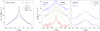 |
Fig. 9 Galactic latitude profiles averaged over the whole longitude range. In the left panel I show IV(100 µm) and the β × Iv(100 µm) templates for the BIPP, FUV, and 1.25 µm bands. In the two panels on the right, I show the profiles for diffuse radiation directly estimated from observations and those from the “literature” and “fit” solutions (see text for details). |
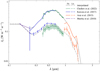 |
Fig. 10 Diffuse starlight component of the LISRF spectrum. I show the “literature” and “fit” estimates together with the interpolated solutions (see text for details). |
5.2 The “fit” solution
As an alternative solution, I constructed a template for  using Eq. (8), the Schlegel et al. (1998) maps for extinction and 7y(100 µm), and the Fitzpatrick (1999) average extinction law. The effects of the βλ corrective term (Eq. (9)) is shown in the left panel of Fig. 3, for a few representative bands: at a shorter λ, the Galactic latitude profile of the template becomes shallower and can describe better the shallow trend of
  derived from observations, without the need for introducing a saturation cut in Iv(100 µm). Thus, the template can be scaled to match, on average, the maps of diffuse emission derived from observations, by using a single scaling factor over the whole dynamic range of Iv(100 µm).
The comparison between the observed profiles and those for the rescaled templates is shown in the right panels of Fig. 9. Despite the crudeness of the modeling, there is a satisfactory agreement in the Pioneer bands. In the FUV,  is very close to the literature estimate. The result in the NUV would be similar if I had subtracted the large zero-level discussed earlier; however, in order to retain all emission, the template is scaled to the full NUV emission. The worse agreement is seen in the DIRBE 1.25 µm band, despite the fact that this analysis is restricted to the galactic plane (b < 40°) to avoid noisy regions. I discuss these issues in the next section.
Finally, I used the scaling factors found for the bands of Fig. 9 to rescale the published spectra. Analogously to the procedure described in the previous section, I called the interpolation over the whole UV-optical-NIR range the “fit” solution (shown in Fig. 10). By construction, the Jλ spectrum in the optical-NIR is higher for the “fit” solution, by about a factor 3. In the next section, I demonstrate the impact of the two different solutions on the total LISRF spectrum.
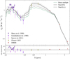 |
Fig. 11 Total LISRF spectrum compared to estimates derived from large-area observations. The bottom panel show the relative difference between observations and synthetic photometry derived from the “fit” solution spectrum. |
6 The total LISRF spectrum: Results and discussion
I added the LISRF spectrum from direct starlight (Sect. 4) to the “literature” and “fit” solutions for the spectrum of diffuse light (Sect. 5) to obtain two estimates of the total LISRF: they are shown in Fig. 11. The two estimates are compared with those values of Jλ presented in Sect. 3 that are obtained (or estimated) on a large fraction of the sky.
As discussed in the previous section, diffuse radiation estimated from the “literature” solution, when added to direct starlight, is not able to reproduce the independent estimates of Jλ in the optical and NIR. The “fit” solution instead is made to pass through (or near) them by construction. For the Pioneer bands, a possible reason for the apparent failure of the “literature” solution could be that the estimates from observations are biased high. As discussed in Appendix A.2, the contribution of bright stars was removed from the distributed Pioneer data; yet the data might still include a significant residual contribution from those objects. As a result, a fraction of direct starlight could have been counted twice, being included in both the recovered emission for V < 6.5 stars and possibly in the available maps including stars with V > 6.5 and diffuse radiation (see Appendix A.2 for details). This uncertainty is included in the large errors shown in Fig. 11. The “literature” solution could be consistent (though marginally) with the βIPP datapoint. However, Jλ in RIPP still requires a contribution from diffuse starlight that the “literature” solution cannot provide.
In the DIRBE 1.25 µm band, the total Jλ is not only higher than the “literature” solution, but also of the “fit” one. In fact, the template for diffuse starlight does not match the estimate based on observations near the galactic center (see the excess emission on the plane in Fig. 9). The reason is shown by the map of Fig. 8: a central structure can be seen, resembling the Galactic bulge (obviously missing from the IRAS-based template). Clearly, the model of Sect. 4 was not sufficient to remove the full direct starlight contribution. This could be the results of highly extinguished stars emitting predominantly in the NIR band (but missing from the Gaia catalog, as discussed in Sect. 4); or to the inaccuracy of the approximation for the spectrum of the redder Gaia stars without APs. The same issue could be the cause for the flat (but noisy) background at high galactic latitude (see Fig. 9). In any case, once the “fit” solution is subtracted, the residual emission accounts only for Jλ ≈ 0.03 W m−3 sr−1 (mostly from the bulge region with |b| < 30°, |l| < 30°). This value is of the order of the error on the full Jλ estimate in this band (Appendix A.1), and about half of the uncertainty estimated in Sect. 4 for the model of direct starlight. Thus, I can still consider the “fit” solution consistent with observations.
Another reason for the failure of the “literature” solution might reside in the smaller dynamic range and spatial coverage of the data used to derive the correlations in the optical and NIR. The bulk of the contribution of diffuse starlight to Jλ comes from low Galactic latitude (≈70% from |b| < 20° in the optical and NIR), while most of the analysis in the literature is done on high Galactic latitude regions, with the exception of Kawara et al. (2017), which do include observation close to the Galactic plane. Also, while here templates are derived after averaging the observations over pixels of ~1° × 1°, the individual observations of Kawara et al. (2017) and Chellew et al. (2022) have field-of-views of few arcsec squared; those of Arai et al. (2015) do cover field-of-views of a few degrees squared (though not continuously, but with a series of thin slits) but are limited to just six high latitude regions. Thus, one might wonder if those correlations describe better variation with Iv(100 µm) at smaller scales than the single template scaled on the whole sky.
The variety of methods also might cause some differences. For example, only Kawara et al. (2017) subtract the extragalac-tic background (though using a value higher than what assumed here, thus causing the steeper latitude gradients of the “literature” profiles in the optical shown in Fig. 9). Chellew et al. (2022) do not explicitly consider the impact of zodiacal light; also, their results have to be scaled by a bias factor in order to reproduce the results of a radiative transfer model of diffuse starlight (Brandt & Draine 2012). Even after applying the correction, the results (and thus the radiative transfer model used to rescale them) are still offset from those of Kawara et al. (2017) and Arai et al. (2015) (see also Fig. 10).
The difference between the two solutions is negligible in the UV, where the correlations from Murthy et al. (2010) was derived on a large fraction of the sky: their results, coupled with the simple model for the saturation with dust extinction, are very similar to the current template-based approach, at least in the FUV, but also in the NUV if the zero-level offset found by Murthy (2014) had been removed.
In the following, the total Jλ including the “fit” solution is adopted as the correct LISRF representation. Since the spectrum is made to pass through the Pioneer datapoints, I require the total uncertainty of the spectrum to match the uncertainty from those observations (for a conservative estimate, I use the larger error for BIPP): this can be achieve by assuming a relative uncertainty of ∼40% for diffuse starlight (added in quadrature to the uncertainty for direct starlight presented in Sect. 4). The same relative error is used for the whole wavelength range and the total is shown with the shaded area in Fig. 11. The total uncertainty in the optical range is 13% (again by construction). In the UV (in the range of the FUV and NUV bands) the uncertainty rises to 16% (because of the higher uncertainty of direct starlight, while the contribution of diffuse starlight is reduced with respect to the optical). This value is lower than the average scatter of the UV datapoints around the “fit” solution, ∼25%, probably due the large calibration uncertainties of the observations. Longer wavelengths, instead, are dominated by direct starlight and the uncertainty is ∼7%, as estimated in Sect. 4; the larger discrepancy of the DIRBE 3.5 µm datapoints might come from the additional contribution of dust in emission (not considered in this analysis). However, radiation in this part of the spectrum constitutes only a minor part of the total energy of the LISRF.
Diffuse starlight contributes on average to ≈20% of the total LISRF in the UV for λ < 0.3 µm, rising to ≈30% in the optical for 0.4 µm < λ < 0.7 µm, then falling in the NIR, with a 10% contribution at 1.25 µm (for the “fit” solution; ≈15, 10 and 5%, respectively, for the “literature” solution). In Fig. 12, I show the Iλ profile predicted for the Gaia G band and the variation of the fraction of diffuse starlight with latitude: beside a central peak, the contribution of diffuse starlight is relatively constant (≈25%) with latitude up to |b| ≈ 50°, dropping to 10% towards the poles (for the “fit” solution).
The new LISRF spectrum is compared with MMP in the top right panel of Fig. 13, while in Table 2 values of Jλ are listed in some representative bands across the UV, optical and NIR spectrum. The differences between the two spectra are significant: the new LISRF is ~20% lower in FUV, and 30%, 35% and up to ~70% higher in G, J and K, corresponding to discrepancies from 2 to 6× the 15% uncertainty claimed by Mathis et al. (1983).
The total flux from the integration of the new spectrum over the whole wavelength range is ∼30% higher than in MMP. Also, the balance between UV and optical-NIR radiation is different: radiation for λ < 0.4 µm constitutes ~10% of the total energy output for the new LISRF, while it is ~20% for MMP. While differences are expected in the optical and NIR, due to the new data not available at the time of the MMP papers, the larger UV output is due to the choice of Mezger et al. (1982) of raising the Gondhalekar et al. (1980) fluxes by 15%, in order to have a better agreement with the data from Henry et al. (1980). On the contrary, the current spectrum estimate agrees better with the original Gondhalekar et al. (1980) values.
Differences between the new LISRF and the model of Draine (2011) are reduced but still significative in the UV (where the model is the same as MMP) and at λ ≈ 1 µm. The total integrated flux of Draine (2011) is slightly higher than the current estimate (and ∼40% higher than MMP), while the contribution to the total of UV radiation at λ < 0.4 µm is ∼15%.
 |
Fig. 12 Galactic latitude profile of lλ, predicted for the Gaia G band, for direct and diffuse starlight, and the total (“fit” solution). The lower panel shows the fractional contribution of diffuse starlight for both “fit” and “literature” solutions. |
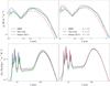 |
Fig. 13 Top row: LISRF from this work (“fit” solution, with its uncertainty), MMP and Draine (2011) (left panel); LISRFs rescaled by the factor U in the legend (right panel). Bottom row: Dust emissivity predicted for the Jones et al. (2017) dust model under different heating conditions. Each bottom panel shows the results for the LISRFs presented in the corresponding upper panel. |
Selected in-band values of the new LISRF vs. MMP.
7 An application of the new ISRF to dust heating
Models for MW dust grains are required to reproduce several observational constraints: one of them is the emissivity (surface brightness per gas column density) of high Galactic-latitude dust (the cirrus) that have been observed from the MIR to the submm by a variety of instruments (for the latest observational constraints see, e.g., Hensley & Draine 2021; Ysard et al. 2024). The most common approach is to assume that the cirrus is heated by the LISRF: for example, several authors have used the MMP model to validate grain mixtures proposed for dust in the diffuse ISM (e.g., Dwek et al. 1997; Li & Draine 2001; Zubko et al. 2004; Compiègne et al. 2011; Siebenmorgen et al. 2014; Jones et al. 2017; Siebenmorgen 2023).
Because of the differences described in the previous section, one should expect that a dust grain mixture will behave differently when heated by each of the LISRFs considered here. I evaluate the dependence of dust emission on the LISRF assumption by using The Heterogeneous dust Evolution Model for Interstellar Solids (THEMIS5) and computing the MIR-to-submm emissivities with the DustEM software6 (Compiègne et al. 2011). The THEMIS model for dust in the diffuse ISM essentially consists of three grain populations: i) hydrogenated amorphous carbon, a-C(:H), grains of large size (typical radius a ≈ 200 nm), with a photo-processed a-C mantle, responsible for extinction/absorption in the optical and making most of the FIR emission at thermal equilibrium; ii) amorphous silicate grains with iron inclusions and a-C mantles, of similar size and contributing to the FIR emission; iii) amorphous carbon grains (a-C) of small size (from 100 down to 0.4 nm), responsible for the rise of extinction for UV radiation end emitting stochastically in the MIR, both in the continuum (I use here λ = 30 µm as a reference) and in the emission bands for 3 ≲ λ/µm ≲ 15 (other models prefer to use the Polycyclic Aromatic Hydrocarbon macro-molecules, PAHs, as the carriers of these features; Draine 2011). For full details on THEMIS, see Jones et al. (2013); here I use the version documented in Jones et al. (2017).
Figure 13 (bottom left panel) shows the emissivity predicted for THEMIS. Overall, the dust model absorbs (and re-emits) 6% more radiation when heated by the LISRF derived in this work (and 17% for Draine 2011) with respect to when MMP is used. The ratios are different with respect to those for the LISRF total fluxes, because of the different spectra of the LISRFs and of the wavelength-dependent absorption and scattering properties of THEMIS (set to match the observational constraints of the average MW extinction law and albedo). At the peak of thermal emission, the emissivity for the newer LISRF is 8% higher than for MMP; 9% smaller at λ = 30 µm, where the emission is due to stochastically heated small grains; and up to 24% smaller within the MIR bands. For the Draine (2011) LISRF the differences are larger at thermal peak (22% more) and reducing when going to shorter wavelengths up to the MIR features (from 11 to just 2% more, accounting for the similar UV spectrum). In the bottom left panel of Fig. 13, I also show with a shaded area the spread in emissivities delimited by the DustEM output obtained when the LISRFs are the lower and upper boundaries of the uncertainties shown in the top left panel. Most of the differences between the various LISRF are within the shaded area, with the notable exception of the MIR bands.
Since THEMIS meets the observational constraints with MMP, the red curve in the bottom-left panel of Fig. 13 is representative of the observed emissivity. If Jones et al. (2017) had used one of the other estimates for the LISRF, they would have needed to change the properties of the dust model (so that the blue-green curves match the red one). For example, when using the LISRF from this work one would need to lower the contribution of large grains responsible for the thermal peak and raise that of the smaller grains dominating the MIR emissivity. For the same grain size distribution and material composition, this could be naively obtained by changing the dust-to-gas ratios of these components, provided that all other observational constraints are met (and not only emissivity).
For their new model, Hensley & Draine (2023) rescale the Draine (2011) LISRF by multiplying it by a constant factor U = 1 .6 at all wavelengths. The rescaling was required in order to have consistency between the energy absorbed by dust in the UV-to-NIR (constrained by the observed extinction law and albedo) and the energy emitted by dust in the MIR-to-submm (constrained by the observed emissivity spectral energy distribution). The necessity of the rescaling implies that the high-latitude cirrus emission is heated by a stronger radiation field than what is measured locally (if the properties adopted in the dust model are correct). A similar conclusion is reached by Ysard et al. (2024) when fitting a newer version of the THEMIS model for diffuse dust: they found that a better match between the model output and the observed dust emissivity is obtained when the MMP LISRF is scaled by a factor7 U = 1.4.
Even without using the models of Hensley & Draine (2023) and Ysard et al. (2024), the impact of the new LISRF can still be tested, following their approach. To start, we can assume that the observed dust emissivity is the same as that derived from the THEMIS version I use, when the heating is provided by the MMP LISRF multiplied by a factor U = 1.4 (Fig. 13, top-right); and that the total energy absorbed from the rescaled MMP LISRF matches the energy emitted by dust (i.e., the integral of the red curve in the bottom-right panel of Fig. 13, for this test). When I use the LISRF derived in this work, I need to multiply it by a factor U ≈ 1 .3 in order to match the same absorbed energy; the factor U is slightly smaller than for MMP, because, as we have seen, slightly more energy is absorbed by the unscaled (i.e., U = 1) new LISRF. I applied the same procedure to the lower and upper boundaries of the uncertainty estimate, by multiplying the former by U = 1.5 and the latter by U = 1.2: given all the spectra are normalized to the same energy values, the reduced shaded area in the top-right panel now reflects only the different uncertainties estimated across the spectrum (larger in UV than in NIR). The corresponding emissivity (and uncertainty) is shown as a green line in the bottom-right panel of Fig. 13: while the total absorbed energy is the same by construction, the emissivity computed using the spectral shape of the new LISRF is slightly higher in the FIR/submm (by 2% at the peak and tending to 1% for the summ) and considerably smaller at shorter wavelengths (by 15% at 30 µm and ≈30% within the MIR bands). Again, as for the output of the unrescaled model (bottom-left panel) I could match the “observed” emissivity (the red curve, for this test), by increasing in the dust model the contribution of small grains relatively to large grains. For the Draine (2011) LISRF, U ≈ 1.2 is needed: the emissivity is 4% higher at the peak (approaching 1% in the submm), 5% lower at 30 µm and ≈12% lower in the MIR.
Hensley & Draine (2023) and Ysard et al. (2024) required their models to match the observational constraints within a maximum discrepancy of 20%. Without changing any of the properties in the dust model, the use of the LISRF derived in this work can result in differences in the predicted dust emis-sivity as high as 30%. Therefore, the impact of the new LISRF should be considered in dust models, in particular for the component of small grains responsible for the continuum and band emission in the MIR.
8 Summary
I reevaluated the spectrum of the LISRF from the UV to the NIR, using Gaia DR3 photometry and stellar atmosphere parameters. The steps of this work can be summarized as follows.
The contribution of direct starlight to the LISRF has been estimated in the three Gaia photometric bands, by summing up the fluxes of all stars in the DR3 catalog and those of nearby, bright objects in the HIPPARCOS catalog that have not been included in DR3.
The full UV-to-NIR spectrum for direct starlight has been computed, using the stellar atmosphere models of Castelli & Kurucz (2003) for Gaia stars with APs, a color-based extrapolation for Gaia stars without APs, and an additional component for the HIPPARCOS stars not in DR3.
The full LISRF including direct and diffuse starlight has been derived in the optical, using Pioneer 10/11 observations, as well as in the NIR, using DIRBE maps. After subtracting the contribution of direct starlight obtained from the Gaia-based spectrum, the maps of the residuals have been used (together with GALEX background maps) as a reference set for the diffuse starlight component of the LISRF.
Correlations found in the literature between diffuse starlight (scattered by dust in the ISM) and IRAS 100 µm emission (from dust at thermal equilibrium) have been rescaled to match the levels in the reference set and used to derive the diffuse starlight spectrum of the LISRF from the UV to the NIR.
Finally, the contribution of both direct and diffuse starlight has been summed to obtain the full LISRF spectrum.
The main results of this study are as follows.
The new LISRF spectrum is redder than that of the standard MMP model of Mathis et al. (1983), being ∼20 lower in the FUV and >30% higher from the optical to the NIR. Also, the total energy emitted over the UV-to-NIR spectrum is ~30% higher than the corresponding MMP value. In the optical/NIR, differences with respect to the Draine (2011) update of MMP are smaller, with the new estimate being at most ∼15% lower (at λ ≈ 1 µm).
Because of the different spectral shape, dust models exposed to the new LISRF can have MIR emissivities by up to 30% lower than in the standard case when the MMP is used as a heating field. This difference could lead to significant changes in the constraints of the population of small grains and of the carriers of the MIR bands.
On average, diffuse radiation scattered by dust in the optical contributes to 25% of Iλ for |b| < 50°. Apparently, the global correlation between dust scattered radiation and dust emission at 100 µm is stronger than what found in the literature mostly at high Galactic latitude, by a factor ∼3 in the optical/NIR.
For the next generation of dust grain models, I recommend the usage of the new LISRF presented in this work. It ought to be complemented with a comparison with results obtained by using the MMP and the less often adopted formulation by Draine (2011).
Data availability
The following data is provided online at the CDS: the Jλ spectrum (total and separate direct and diffuse components); the Iλ spectral cubes; and the Pioneer Iλ maps, including the contribution of bright stars. Data are available at the CDS via anonymous ftp to cdsarc.cds.unistra.fr (130.79.128.5) or via https://cdsarc.cds.unistra.fr/viz-bin/cat/J/A+A/691/A330.
Acknowledgements
I am greatly indebted to Elena Pancino for her exquisite guidance through the details of Gaia and its data products. I also thank L. Magrini and S. Zibetti for many helpful suggestions on the modeling of stellar spectra, Y. Matsuoka for details on the correlations between scattered starlight and infrared radiation, and B. Draine for helpful discussions. This work has made use of data from the European Space Agency (ESA) mission Gaia (https://www.cosmos.esa.int/gaia), processed by the Gaia Data Processing and Analysis Consortium (DPAC, https://www.cosmos.esa.int/web/gaia/dpac/consortium). Funding for the DPAC has been provided by national institutions, in particular the institutions participating in the Gaia Multilateral Agreement. Part of this work is based on archival data, software or online services provided by the Space Science Data Center, a facility maintained by the Italian Space Agency. This research has made use of the SIMBAD database and of the SIM-BAD catalog access tool, operated at CDS, Strasbourg, France. I acknowledge the use of data provided by the Centre d’Analyse de Données Etendues (CADE), a service of IRAP-UPS/CNRS (http://cade.irap.omp.eu, Paradis et al. 2012). I acknowledge the use of the Legacy Archive for Microwave Background Data Analysis (LAMBDA), part of the High Energy Astrophysics Science Archive Center (HEASARC). HEASARC/LAMBDA is a service of the Astrophysics Science Division at the NASA Goddard Space Flight Center. For the analysys and visualization of the results, I used Python (Van Rossum & Drake 2009) and its packages astropy (Astropy Collaboration 2018); dust_extinction (Gordon 2023); healpy (Zonca et al. 2019); matplotlib (Hunter 2007); numpy (Harris et al. 2020); pandas (Wes McKinney 2010); pysynphot (STScI Development Team 2013).
Appendix A New LISRF determinations
I describe here new estimates of Jλ in the NIR (obtained from COBE-DIRBE data) and in the optical (from Pioneer-IPPs data).
A.1 COBE-DIRBE
The DIRBE instrument aboard the COBE satellite observed the whole sky in 10 bands between the NIR (from 1.25 µm) and the FIR (to 240 µm; Hauser et al. 1998). In this work, I use the Zodi-Subtracted Mission Average (ZSMA) maps at 1.25, 2.2, 3.5 µm (Arendt et al. 1998), available in HEALPix format at the “Centre d’Analyse de Données Etendues” (CADE)8. The maps were color corrected from the original calibration convention, assuming a blackbody spectrum with T = 3000K (i.e., the NIR dilute blackbody in MMP; see Sect. 3) and the DIRBE color-correction software available at the Legacy Archive for Microwave Background Data Analysis (LAMBDA)9.
The DIRBE Iλ map at 2.2 µm is shown in Fig. A.1. Jλ for the three DIRBE bands considered here is listed in Table A.1. The errors are dominated by the calibration uncertainty (3.1%; Hauser et al. 1998).
A.2 Pioneer-IPPs
The Pioneer 10 and 11 probes were equipped with two identical instruments, the Imaging Photopolarimeters (IPPs; Weinberg et al. 1973), observing in a blue band (BIPP, λ = 0.437 µm) and a red band (RIPP, λ = 0.644 µm). On a few occasions, the IPPs mapped a considerable part of the whole sky while the probes were spinning around their cruise directions. This resulted in complex observation patterns, with the field of view of the various pointings (FOVs) ranging from 7.5 to 18 degree2. Furthermore, the patterns do not overlap, since the probes gradually changed cruise directions (Toller et al. 1987; Gordon et al. 1998;Leinert et al. 1998).
The data was distributed after removing the contribution of the brighter stars, estimated using the entries in the Yale Bright Stars Catalog and in the USNO Photoelectric Catalog (for additional stars with V < 8): the choice is equivalent to select all stars with V < 6.5 (Toller et al. 1987). In order to recover this contribution, I used the HIPPARCOS catalog to select V < 6.5 stars; they are ∼8800, while the original list subtracted from the IPP maps had ∼12500 entries (Leinert et al. 1998). For these stars, I converted the HlPPARCOS/Tycho BT and VT magnitudes from the catalog to those in the IPP system (with the transformations of Matsuoka et al. 2011). Finally, fluxes in physical units were obtained using the zero points from Gordon et al. (1998) and summed over a HEALPix grid. The reconstructed map of Iλ for the bright stars is shown in Fig. A.2 for the BIPP band; Jλ values are listed in Table A.1. For an additional check, I downloaded more recent versions of the Yale Bright Stars and Photometric catalogs (Hoffleit & Jaschek 1991 and Mermilliod 1987, respectively) from SIMBAD10. After applying the V < 8 cut, the merged catalog contains ~ 17000 stars. I converted the tabulated Johnson B and V magnitudes to those in the HIPPAROS/Tycho system (using the transformations in Pancino et al. 2022); and then proceeded as above for the HIPPARCOS catalog. The difference with the previous estimate is ≲ 15%; I adopt it as the uncertainty in the estimate of Jλ, accounting for the magnitude transformations and the differences between the stellar catalogs I used and the original catalog used for star removal.
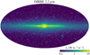 |
Fig. A.1 Iλ at 2.2 µm from DIRBE. |
New LISRF determinations.
Gordon et al. (1998) produced maps from eleven IPP observations taken in 1973–74, when the Pioneer’s were sufficiently distant from the Sun and the contamination from interplanetary dust negligible. Because of the subtraction of bright stars, the IPP maps should include the total radiation from all stars with V > 6.5, plus the diffuse radiation scattered by dust (or any other source of radiation beyond stars, such as the dust-related extended red emission investigated by Gordon et al. 1998). I converted the Gordon et al. (1998) maps11 to the current format to derive Iλ (shown in Fig. A.2 for BIPP); and Jλ, after filling the regions unobserved by the IPPs with the average Iλ trend with latitude (Table A.1). Before producing the maps, Gordon et al. (1998) filtered the original FOV data to remove observations close to the Sun and fluxes corrupted during data transmission; but also data with “incorrect subtraction of bright stars”. In order to check the importance of the incorrect star subtraction in the original dataset, I produced new maps directly from the FOV list provided by the authors, without applying filtering. Curiously, in the unfiltered maps many bright stars are visible, even as bright as V ≤ 2. Some of them can still be seen, as residuals, in the maps of Gordon et al. (1998): for example, when comparing the two maps in Fig. A.2, one can identify easily α Boo (Arcturus, near the central meridian towards the Galactic North Pole) and α Car (Canopus, below the Galactic plane on the top-right of the Large Magellanic Cloud). From the unfiltered maps, I can derive Jλ values higher than those from the maps of Gordon et al. (1998), by 15% and 7% in the BIPP and RIPP bands, respectively. The difference between the unfiltered Pioneer maps, which still apparently includes bright stars, and the maps of Gordon et al. (1998), where most (thought not all) the flux from bright stars is removed, are used as a conservative estimates of the uncertainties on IPP estimates of Jλ, to which I added a further 8% calibration uncertainty (Hanner et al. 1976). The adopted error on the IPP-based Jλ is given in Table A.1. Finally, I sum the contribution of the bright stars and of the IPP maps to derive the total estimates of Jλ (Table A.1).
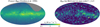 |
Fig. A.2 Pioneer BIPP map from Gordon et al. (1998) (left). Reconstructed contribution from V ≤ 6.5 stars using the HIPPARCOS catalog (right), smoothed with a FWHM=4° Gaussian (to match approximately the resolution of IPP maps). |
Appendix B Validation of synthetic spectra
The reliability of the synthetic spectra obtained in Sect. 4 is controlled by deriving Jλ for the cross-matches between the Gaia/HIPPARCOS catalogs and other independent photometric catalogs: the value obtained by the summation of the stellar fluxes in each photometric band of the independent catalog is compared with the synthetic photometry derived over the same band from the Jλ spectrum. I use the TD-1 catalog (Thompson et al. 1978) in the UV, the 2MASS PointSource Catalog (Skrutskie et al. 2006) in the NIR, for Gaia and HIPPARCOS-derived spectra, and BVJHK photometry from SIMBAD, for HIPPARCOS only.
B.1 Gaia
Using SIMBAD, I searched the Gaia DR3 identifier for each star in the TD-1 catalog: out of the ~31000 stars in TD-1, I found a counterpart in Gaia for ~29500; the selection further restricts to ~19000 stars if only Gaia AP objects are considered for which the spectrum can be estimated directly (see Sect. 4.1). The Jλ spectrum for this selection, together with synthetic and observed datapoints, is shown in Fig. B.1. Judging on the difference, I adopt for the spectrum a relative error of 16% in this range. Even though the spectrum for this selection is on average only 40% of the full Gaia (AP + non-AP extrapolation) spectrum, I assume that the same relative error can be applied in this range for the latter.
The DR3 cross-match between 2MASS and Gaia contains ∼330 million best-neighbor counterparts to Gaia AP stars. Again the total spectrum, the synthetic estimate and the result from flux summation are shown in Fig. B.1. In this range, the difference reduces to 7%. The total spectrum for this selection is very close to the full Gaia AP spectrum across all wavelengths (also shown in the figure); in the NIR, it is 40% of the full Gaia (AP + non-AP extrapolation) spectrum.
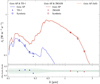 |
Fig. B.1 Jλ for the cross-matches between Gaia AP stars and the TD-1 and 2MASS catalogs. I show the spectrum, synthetic photometry and observation for each cross-match. I also show for comparison the Gaia AP spectrum. The relative difference between observations and synthetic photometry is shown in the bottom panel. The shaded area highlights the uncertainty I adopt for the estimate. |
B.2 HIPPARCOS
According to SIMBAD, there are ~23500 TD-1 stars with an HIPPARCOS identifier. From the difference between synthetic and observed datapoints in Fig. B.2, I adopt for the spectrum a relative error of 17% in this range. In this case, the spectrum for the selection is 2.5× higher than the one I derive in Sect. 4.2 for the HIPPARCOS stars not included in the Gaia catalog, which are only ~1500.
Using SIMBAD, I found a complete set of BVJHK photometry for ~94% of the HIPPARCOS stars. Most of the recovered photometry comes from the Tycho-2 catalog (Høg et al. 2000, for B and V) and the 2MASS PointSource Catalog (Skrutskie et al. 2006, for J, H and K). The comparison between synthetic and observed datapoints (see Fig. B.2) suggests an overall uncertainty of the spectrum of 10% over the optical/NIR range. In this case, the spectrum is ~ 6× higher than for the selection used in Sect. 4.2
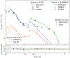 |
Fig. B.2 Same as Fig. B.1, but for the cross-matches between HIPPARCOS and the TD1 catalog and a SIMBAD photometry search. I also show Jλ in the Gaia bands derived independently from HIPPARCOS and Gaia, for the official cross-match between the two catalogs; and the independent spectra estimated from matched HIPPARCOS and Gaia AP stars. For the HIPPARCOS/Gaia comparison in the lower panel (i.e., black symbols and orange line), the reference values (i.e., Synth.) are the Gaia photometry and spectrum. |
B.3 HIPPARCOS vs Gaia
I also checked the accuracy in the derivation of Gaia-band photometry from the original HIPPARCOS photometry (Sect. 2.2). In Fig. B.2 I show the comparison between Jλ in the Gaia bands, obtained from HIPPARCOS fluxes and directly from Gaia fluxes, for the official best-neighbor cross-match between the two catalogs (~100000 stars). The relative difference is within 2% (See also Sect. 2.2 and Table 1).
In analogy, I checked the total spectra derived independently from the two ways described in Sect. 4, for a subsample restricted to the stars with Gaia APs (∼65000 stars). The cross-match gives the opportunity of comparing the values of A0 from Gaia, derived self-consistently with the other APs, and those computed from the optical-NIR photometry available for HIPPARCOS stars, after assuming the parameters for stellar atmospheres derived from SIMBAD and the HIPPARCOS catalog (see Sect. 4.2). The comparison is shown in Fig. B.3: there is a general agreement between the two estimates, but with a large scatter, even for the best case in which all stellar parameters of HIPPARCOS stars are retrieved from the independent dataset, and A0 is derived from the average of six colors. The scatter is probably due to the extinction-temperature degeneracy: if the predicted intrinsic stellar spectrum is, for instance, too blue, the corresponding Ao is biased towards higher values in order to compensate and match the observed photometry. While this issue affects also AP estimates (Andrae et al. 2023), it is likely more important in the independent, non self-consistent, estimates based on SIMBAD and the HIPPARCOS catalog. Nevertheless, the sum over the whole cross-match catalog results in total spectra (also shown in Fig. B.2) which are still within the uncertainties already assumed in this section. Averaging over a large number of objects (most of which have small A0 values because of their closeness) reduces the effects of the scatter in A0 (and of the differences between Gaia APs and the independent stellar parameters). Only for λ ≤ 0.11µm the uncertainties are larger, probably because of the issues discussed so-far, but also because of the different gridding in the table of model spectra used for the HIPPARCOS estimate. Attaching more confidence to the Gaia-derived spectra, I raise the uncertainty for HIPPARCOS spectrum in this range accordingly.
 |
Fig. B.3 Comparison between A0 values from the Gaia AP dataset and those derived from independent stellar parameters from the SIMBAD database and the HIPPARCOS catalog. Red datapoints show all stars in the Gaia-HIPPARCOS cross-match, blue ones those with the best independent dataset (all stellar parameters recovered and extinction derived from six colors; see Sect. 4.2 for details). The dashed line shows the 1-1 correspondence. |
References
- Allen, C. W. 1973, Astrophysical Quantities, 3rd edn. (The Athlon Press, University of London) [Google Scholar]
- Andrae, R., Fouesneau, M., Sordo, R., et al. 2023, A&A, 674, A27 [CrossRef] [EDP Sciences] [Google Scholar]
- Arai, T., Matsuura, S., Bock, J., et al. 2015, ApJ, 806, 69 [NASA ADS] [CrossRef] [Google Scholar]
- Arendt, R. G., Odegard, N., Weiland, J. L., et al. 1998, ApJ, 508, 74 [NASA ADS] [CrossRef] [Google Scholar]
- Astropy Collaboration (Price-Whelan, A. M., et al.) 2018, AJ, 156, 123 [Google Scholar]
- Boggess, N. W., Mather, J. C., Weiss, R., et al. 1992, ApJ, 397, 420 [Google Scholar]
- Brandt, T. D., & Draine, B. T. 2012, ApJ, 744, 129 [Google Scholar]
- Castelli, F., & Kurucz, R. L. 2003, in Modelling of Stellar Atmospheres, 210, eds. N. Piskunov, W. W. Weiss, & D. F. Gray, A20 [NASA ADS] [Google Scholar]
- Chellew, B., Brandt, T. D., Hensley, B. S., Draine, B. T., & Matthaey, E. 2022, ApJ, 932, 112 [CrossRef] [Google Scholar]
- Compiègne, M., Verstraete, L., Jones, A., et al. 2011, A&A, 525, A103 [Google Scholar]
- Creevey, O. L., Sordo, R., Pailler, F., et al. 2023, A&A, 674, A26 [NASA ADS] [CrossRef] [EDP Sciences] [Google Scholar]
- Désert, F. X., Boulanger, F., & Puget, J. L. 1990, A&A, 237, 215 [NASA ADS] [Google Scholar]
- de Zeeuw, P. T., Hoogerwerf, R., de Bruijne, J. H. J., Brown, A. G. A., & Blaauw, A. 1999, AJ, 117, 354 [Google Scholar]
- Draine, B. T. 2011, Physics of the Interstellar and Intergalactic Medium (Princeton University Press) [Google Scholar]
- Draine, B. T., Dale, D. A., Bendo, G., et al. 2007, ApJ, 663, 866 [NASA ADS] [CrossRef] [Google Scholar]
- Driver, S. P., Andrews, S. K., Davies, L. J., et al. 2016, ApJ, 827, 108 [CrossRef] [Google Scholar]
- Dwek, E., Arendt, R. G., Fixsen, D. J., et al. 1997, ApJ, 475, 565 [NASA ADS] [CrossRef] [Google Scholar]
- Edelstein, J., Korpela, E. J., Adolfo, J., et al. 2006, ApJ, 644, L159 [NASA ADS] [CrossRef] [Google Scholar]
- ESA Pubblication division 1997, ESA Special Publication, 1200 [Google Scholar]
- Evans, D. W., Eyer, L., Busso, G., et al. 2023, A&A, 674, A4 [NASA ADS] [CrossRef] [EDP Sciences] [Google Scholar]
- Fitzpatrick, E. L. 1999, PASP, 111, 63 [Google Scholar]
- Gaia Collaboration (Prusti, T., et al.) 2016, A&A, 595, A1 [NASA ADS] [CrossRef] [EDP Sciences] [Google Scholar]
- Gaia Collaboration (Brown, A. G. A., et al.) 2018, A&A, 616, A1 [NASA ADS] [CrossRef] [EDP Sciences] [Google Scholar]
- Gaia Collaboration (Brown, A. G. A., et al.) 2021, A&A, 649, A1 [NASA ADS] [CrossRef] [EDP Sciences] [Google Scholar]
- Gaia Collaboration (Vallenari, A., et al.) 2023, A&A, 674, A1 [NASA ADS] [CrossRef] [EDP Sciences] [Google Scholar]
- Galliano, F., Hony, S., Bernard, J.-P., et al. 2011, A&A, 536, A88 [NASA ADS] [CrossRef] [EDP Sciences] [Google Scholar]
- Gondhalekar, P. M. 1990, in The Galactic and Extragalactic Background Radiation, 139, eds. S. Bowyer, & C. Leinert, 49 [NASA ADS] [CrossRef] [Google Scholar]
- Gondhalekar, P. M., Phillips, A. P., & Wilson, R. 1980, A&A, 85, 272 [NASA ADS] [Google Scholar]
- Gordon, K. 2023, https://doi.org/10.5281/zenodo.7799360 [Google Scholar]
- Gordon, K. D., Witt, A. N., & Friedmann, B. C. 1998, ApJ, 498, 522 [NASA ADS] [CrossRef] [Google Scholar]
- Górski, K. M., Hivon, E., Banday, A. J., et al. 2005, ApJ, 622, 759 [Google Scholar]
- Habing, H. J. 1968, Bull. Astron. Inst. Netherlands, 19, 421 [Google Scholar]
- Hanner, M. S., Sparrow, J. G., Weinberg, J. L., & Beeson, D. E. 1976, in Interplanetary Dust and Zodiacal Light, 48, eds. H. Elsaesser, & H. Fechtig, (Springer), 29 [NASA ADS] [CrossRef] [Google Scholar]
- Harris, C. R., Millman, K. J., van der Walt, S. J., et al. 2020, Nature, 585, 357 [NASA ADS] [CrossRef] [Google Scholar]
- Hauser, M. G., Arendt, R. G., Kelsall, T., et al. 1998, ApJ, 508, 25 [Google Scholar]
- Hayakawa, S., Ito, K., Matsumoto, T., Murakami, H., & Uyama, K. 1978, PASJ, 30, 369 [NASA ADS] [Google Scholar]
- Henry, R. C., Weinstein, A., Feldman, P. D., Fastie, W. G., & Moos, H. W. 1975, ApJ, 201, 613 [NASA ADS] [CrossRef] [Google Scholar]
- Henry, R. C., Swandic, J. R., Shulman, S. D., & Fritz, G. 1977, ApJ, 212, 707 [NASA ADS] [CrossRef] [Google Scholar]
- Henry, R. C., Anderson, R. C., & Fastie, W. G. 1980, ApJ, 239, 859 [NASA ADS] [CrossRef] [Google Scholar]
- Hensley, B. S., & Draine, B. T. 2021, ApJ, 906, 73 [NASA ADS] [CrossRef] [Google Scholar]
- Hensley, B. S., & Draine, B. T. 2023, ApJ, 948, 55 [Google Scholar]
- Hobbs, D., Brown, A., Høg, E., et al. 2021, Exp. Astron., 51, 783 [NASA ADS] [CrossRef] [Google Scholar]
- Hoffleit, D., & Jaschek, C. 1991, The Bright Star Catalogue (New Haven) [Google Scholar]
- Høg, E., Fabricius, C., Makarov, V. V., et al. 2000, A&A, 355, L27 [Google Scholar]
- Hohle, M. M., Neuhäuser, R., & Tetzlaff, N. 2008, New A Rev., 52, 405 [NASA ADS] [CrossRef] [Google Scholar]
- Hunter, J. D. 2007, Comput. Sci. Eng., 9, 90 [NASA ADS] [CrossRef] [Google Scholar]
- Ienaka, N., Kawara, K., Matsuoka, Y., et al. 2013, ApJ, 767, 80 [Google Scholar]
- Jones, A. P. 2009, A&A, 500, 277 [NASA ADS] [CrossRef] [EDP Sciences] [Google Scholar]
- Jones, A. P., Fanciullo, L., Köhler, M., et al. 2013, A&A, 558, A62 [NASA ADS] [CrossRef] [EDP Sciences] [Google Scholar]
- Jones, A. P., Köhler, M., Ysard, N., Bocchio, M., & Verstraete, L. 2017, A&A, 602, A46 [NASA ADS] [CrossRef] [EDP Sciences] [Google Scholar]
- Kawara, K., Matsuoka, Y., Sano, K., et al. 2017, PASJ, 69, 31 [NASA ADS] [CrossRef] [Google Scholar]
- Leinert, C., Bowyer, S., Haikala, L. K., et al. 1998, A&AS, 127, 1 [NASA ADS] [CrossRef] [EDP Sciences] [Google Scholar]
- Li, A., & Draine, B. T. 2001, ApJ, 554, 778 [Google Scholar]
- Lillie, C. F. 1968, PhD thesis, University of Wisconsin System, USA [Google Scholar]
- Marrese, P. M., Marinoni, S., Fabrizio, M., & Altavilla, G. 2019, A&A, 621, A144 [NASA ADS] [CrossRef] [EDP Sciences] [Google Scholar]
- Masana, E., Carrasco, J. M., Bará, S., & Ribas, S. J. 2021, MNRAS, 501, 5443 [NASA ADS] [CrossRef] [Google Scholar]
- Mathis, J. S., Mezger, P. G., & Panagia, N. 1983, A&A, 128, 212 [NASA ADS] [Google Scholar]
- Matsuoka, Y., Ienaka, N., Kawara, K., & Oyabu, S. 2011, ApJ, 736, 119 [NASA ADS] [CrossRef] [Google Scholar]
- Mermilliod, J. C. 1987, A&AS, 71, 413 [Google Scholar]
- Mezger, P. G., Mathis, J. S., & Panagia, N. 1982, A&A, 105, 372 [NASA ADS] [Google Scholar]
- Miville-Deschênes, M., & Lagache, G. 2005, ApJS, 157, 302 [CrossRef] [Google Scholar]
- Murthy, J. 2014, ApJS, 213, 32 [Google Scholar]
- Murthy, J., Henry, R. C., & Sujatha, N. V. 2010, ApJ, 724, 1389 [NASA ADS] [CrossRef] [Google Scholar]
- Murthy, J., Henry, R. C., & Overduin, J. 2023, J. Astrophys. Astron., 44, 82 [NASA ADS] [CrossRef] [Google Scholar]
- Nersesian, A., Xilouris, E. M., Bianchi, S., et al. 2019, A&A, 624, A80 [NASA ADS] [CrossRef] [EDP Sciences] [Google Scholar]
- Neugebauer, G., Habing, H. J., van Duinen, R., et al. 1984, ApJ, 278, L1 [NASA ADS] [CrossRef] [Google Scholar]
- Pancino, E., Marrese, P. M., Marinoni, S., et al. 2022, A&A, 664, A109 [NASA ADS] [CrossRef] [EDP Sciences] [Google Scholar]
- Paradis, D., Dobashi, K., Shimoikura, T., et al. 2012, A&A, 543, A103 [NASA ADS] [CrossRef] [EDP Sciences] [Google Scholar]
- Perryman, M. A. C., Lindegren, L., Kovalevsky, J., et al. 1997, A&A, 323, L49 [Google Scholar]
- Pilbratt, G. L., Riedinger, J. R., Passvogel, T., et al. 2010, A&A, 518, L1 [NASA ADS] [CrossRef] [EDP Sciences] [Google Scholar]
- Planck Collaboration I. 2011, A&A, 536, A1 [NASA ADS] [CrossRef] [EDP Sciences] [Google Scholar]
- Riello, M., De Angeli, F., Evans, D. W., et al. 2021, A&A, 649, A3 [NASA ADS] [CrossRef] [EDP Sciences] [Google Scholar]
- Sano, K., & Matsuura, S. 2017, ApJ, 849, 31 [NASA ADS] [CrossRef] [Google Scholar]
- Sano, K., Kawara, K., Matsuura, S., et al. 2016, ApJ, 818, 72 [CrossRef] [Google Scholar]
- Schlegel, D. J., Finkbeiner, D. P., & Davis, M. 1998, ApJ, 500, 525 [Google Scholar]
- Seon, K.-I., Edelstein, J., Korpela, E., et al. 2011, ApJS, 196, 15 [NASA ADS] [CrossRef] [Google Scholar]
- Siebenmorgen, R. 2023, A&A, 670, A115 [NASA ADS] [CrossRef] [EDP Sciences] [Google Scholar]
- Siebenmorgen, R., Voshchinnikov, N. V., & Bagnulo, S. 2014, A&A, 561, A82 [NASA ADS] [CrossRef] [EDP Sciences] [Google Scholar]
- Skrutskie, M. F., Cutri, R. M., Stiening, R., et al. 2006, AJ, 131, 1163 [NASA ADS] [CrossRef] [Google Scholar]
- Straizys, V., & Kuriliene, G. 1981, Ap&SS, 80, 353 [CrossRef] [Google Scholar]
- STScI Development Team 2013, pysynphot: Synthetic photometry software package, Astrophysics Source Code Library [record ascl:1303.023] [Google Scholar]
- Thompson, G. I., Nandy, K., Jamar, C., et al. 1978, Catalogue of stellar ultraviolet fluxes : a compilation of absolute stellar fluxes measured by the Sky Survey Telescope (S2/68) aboard the ESRO satellite TD-1 (Science Research Council) [Google Scholar]
- Tielens, A. G. G. M., & Hollenbach, D. 1985, ApJ, 291, 722 [Google Scholar]
- Toller, G. N. 1990, in The Galactic and Extragalactic Background Radiation, 138, eds. S. Bowyer, & C. Leinert, 21 [Google Scholar]
- Toller, G., Tanabe, H., & Weinberg, J. L. 1987, A&A, 188, 24 [NASA ADS] [Google Scholar]
- van Leeuwen, F., de Bruijne, J., Babusiaux, C., et al. 2022, Gaia DR3 documentation (European Space Agency; Gaia Data Processing and Analysis Consortium) [Google Scholar]
- Van Rossum, G., & Drake, F. L. 2009, Python 3 Reference Manual (Scotts Valley, CA: CreateSpace) [Google Scholar]
- Weinberg, J. L., Hanner, M. S., Mann, H. M., Hutchison, P. B., & Fimmel, R. 1973, Space Res. Conf., 2, 1187 [NASA ADS] [Google Scholar]
- Weinberg, J. L., Hanner, M. S., Beeson, D. E., DeShields, L. M. I. I., & Green, B. A. 1974, J. Geophys. Res., 79, 3665 [NASA ADS] [CrossRef] [Google Scholar]
- Wes McKinney 2010, in Proceedings of the 9th Python in Science Conference, eds. S. van der Walt, & J. Millman, 56 [CrossRef] [Google Scholar]
- Witt, A. N., & Johnson, M. W. 1973, ApJ, 181, 363 [NASA ADS] [CrossRef] [Google Scholar]
- Ysard, N., Jones, A. P., Guillet, V., et al. 2024, A&A, 684, A34 [NASA ADS] [CrossRef] [EDP Sciences] [Google Scholar]
- Zonca, A., Singer, L., Lenz, D., et al. 2019, J. Open Source Softw., 4, 1298 [Google Scholar]
- Zubko, V., Dwek, E., & Arendt, R. G. 2004, ApJS, 152, 211 [NASA ADS] [CrossRef] [Google Scholar]
Alternatively, the LISRF can be written in terms of energy density, uλ = 4πJλ/c (Draine 2011).
Unless otherwise specified, all Gaia products used in this work, as well as the HIPPARCOS catalog, were downloaded from the Gaia ESA Archive: https://gea.esac.esa.int/archive
Ysard et al. (2024) and the DustEM code call this factor G0. Usually, the name G0 is adopted for the ratio between the total energy radiated over the photon energy range [6,13.6] eV (i.e., [0.0912,0.2] µm) and the same value from the theoretical estimate of the ISRF in the ‘typical’ ISM made by Habing (1968; see also, Tielens & Hollenbach 1985). In units of the Habing flux, it is G0 = 1.14 for the MMP (Draine 2011) and G0 = 0.8 for the current LISRF, accounting for its lower UV output. For simplicity, DustEM sets G0 = 1 for the MMP. Also, the shape of the rescaled spectrum is kept fixed, and thus G0 and U are equivalent (see also Compiègne et al. 2011).
I used the 1st iteration maps and the pre-processed information on the photometry and position of each FOV, available at https://karllark.github.io/data_pioneer10_11_ipp.html.
All Tables
Contribution of direct starlight to the LISRF in Gaia bands, plus estimates for other samples.
All Figures
|
Fig. 1 Jλ vs. Gaia magnitudes, for stars in the Gaia and HIPPARCOS catalogs, and for HIPPARCOS stars with no Gaia counterpart. |
| In the text | |
|
Fig. 2 G-band surface brightness, IG, from the Gaia DR3 catalog (left) and from the HIPPARCOS stars not in DR3 (right). To ease the visualization of the HIPPARCOS contribution, both maps are been smoothed with a Gaussian of FWHM equal to the pixel size. All maps in this work are shown in Galactic coordinates and Mollweide projection (the extent of each map being delimited by Galactic latitude b = −90° at bottom and b = 90° at top, and by Galactic longitude l = −180° at right and l = 180° at left, respectively). |
| In the text | |
|
Fig. 3 Comparison between the Gaia/HIPPARCOS estimates and MMP. Also shown: the observational constraints of MMP (listed in the bottom-left legend); synthetic photometry of the MMP model over the Gaia bands; the Draine (2011) update based on DIRBE full sky data; our estimates from Pioneer 10/11 data; and the more recent UV estimates from Seon et al. (2011). See main text and Appendix A for details. |
| In the text | |
|
Fig. 4 Direct starlight component of the LISRF spectrum. Upper panel: Total spectrum, the spectrum of Gaia AP stars, the recovered spectrum of Gaia non-AP stars, and the spectrum of the HIPPARCOS stars not included in the Gaia catalog. For the total spectrum (and for the Gaia AP com-ponent) I also plot the synthetic Jλ values in the Gaia bands together with the esti-mates from the direct flux summation. I also show observational UV and NIR estimates and the corresponding synthetic photome-try (for the full spectrum only). The relative difference between observations and syn-thetic photometry is shown in the bottom panel. The shaded area refers to the esti-mated uncertainty for the total spectrum (see text for details). |
| In the text | |
|
Fig. 5 JG vs. G (top) and vs. GBP – GRP (bottom), for Gaia stars with and without APs. |
| In the text | |
|
Fig. 6 Predicted Iλ from direct starlight at 0.15 µm and 2.2 µm. Maps have been smoothed with a Gaussian of FWHM=0.7° to match the resolution of DIRBE (and approximately that of the map in Seon et al. 2011). |
| In the text | |
|
Fig. 7 Profiles in the DIRBE 2.2 µm band, along Galactic longitude l (averaged for |b| < 15°) and Galactic latitude b (averaged over the whole l range). |
| In the text | |
|
Fig. 8 Maps of |
| In the text | |
|
Fig. 9 Galactic latitude profiles averaged over the whole longitude range. In the left panel I show IV(100 µm) and the β × Iv(100 µm) templates for the BIPP, FUV, and 1.25 µm bands. In the two panels on the right, I show the profiles for diffuse radiation directly estimated from observations and those from the “literature” and “fit” solutions (see text for details). |
| In the text | |
|
Fig. 10 Diffuse starlight component of the LISRF spectrum. I show the “literature” and “fit” estimates together with the interpolated solutions (see text for details). |
| In the text | |
|
Fig. 11 Total LISRF spectrum compared to estimates derived from large-area observations. The bottom panel show the relative difference between observations and synthetic photometry derived from the “fit” solution spectrum. |
| In the text | |
|
Fig. 12 Galactic latitude profile of lλ, predicted for the Gaia G band, for direct and diffuse starlight, and the total (“fit” solution). The lower panel shows the fractional contribution of diffuse starlight for both “fit” and “literature” solutions. |
| In the text | |
|
Fig. 13 Top row: LISRF from this work (“fit” solution, with its uncertainty), MMP and Draine (2011) (left panel); LISRFs rescaled by the factor U in the legend (right panel). Bottom row: Dust emissivity predicted for the Jones et al. (2017) dust model under different heating conditions. Each bottom panel shows the results for the LISRFs presented in the corresponding upper panel. |
| In the text | |
|
Fig. A.1 Iλ at 2.2 µm from DIRBE. |
| In the text | |
|
Fig. A.2 Pioneer BIPP map from Gordon et al. (1998) (left). Reconstructed contribution from V ≤ 6.5 stars using the HIPPARCOS catalog (right), smoothed with a FWHM=4° Gaussian (to match approximately the resolution of IPP maps). |
| In the text | |
|
Fig. B.1 Jλ for the cross-matches between Gaia AP stars and the TD-1 and 2MASS catalogs. I show the spectrum, synthetic photometry and observation for each cross-match. I also show for comparison the Gaia AP spectrum. The relative difference between observations and synthetic photometry is shown in the bottom panel. The shaded area highlights the uncertainty I adopt for the estimate. |
| In the text | |
|
Fig. B.2 Same as Fig. B.1, but for the cross-matches between HIPPARCOS and the TD1 catalog and a SIMBAD photometry search. I also show Jλ in the Gaia bands derived independently from HIPPARCOS and Gaia, for the official cross-match between the two catalogs; and the independent spectra estimated from matched HIPPARCOS and Gaia AP stars. For the HIPPARCOS/Gaia comparison in the lower panel (i.e., black symbols and orange line), the reference values (i.e., Synth.) are the Gaia photometry and spectrum. |
| In the text | |
|
Fig. B.3 Comparison between A0 values from the Gaia AP dataset and those derived from independent stellar parameters from the SIMBAD database and the HIPPARCOS catalog. Red datapoints show all stars in the Gaia-HIPPARCOS cross-match, blue ones those with the best independent dataset (all stellar parameters recovered and extinction derived from six colors; see Sect. 4.2 for details). The dashed line shows the 1-1 correspondence. |
| In the text | |
Current usage metrics show cumulative count of Article Views (full-text article views including HTML views, PDF and ePub downloads, according to the available data) and Abstracts Views on Vision4Press platform.
Data correspond to usage on the plateform after 2015. The current usage metrics is available 48-96 hours after online publication and is updated daily on week days.
Initial download of the metrics may take a while.