| Issue |
A&A
Volume 691, November 2024
|
|
|---|---|---|
| Article Number | A259 | |
| Number of page(s) | 11 | |
| Section | Extragalactic astronomy | |
| DOI | https://doi.org/10.1051/0004-6361/202450544 | |
| Published online | 19 November 2024 | |
Comparing the interstellar and circumgalactic origin of gas in the tails of jellyfish galaxies
1
Institut für Physik und Astronomie, Universität Potsdam, Karl-Liebknecht-Str. 24/25, 14476 Golm, Germany
2
Leibniz-Institut für Astrophysik Potsdam (AIP), An der Sternwarte 16, 14482 Potsdam, Germany
⋆ Corresponding author; This email address is being protected from spambots. You need JavaScript enabled to view it.
Received:
29
April
2024
Accepted:
26
September
2024
Abstract
Simulations and observations have found long tails in ‘jellyfish galaxies’, which are commonly thought to originate from ram-pressure stripped gas of the interstellar medium (ISM) in the immediate galactic wake. At larger distances from the galaxy, the long tails have been claimed to form in situ, owing to thermal instability and fast radiative cooling of mixed ISM and intracluster medium (ICM). In this paper, we use magnetohydrodynamical wind tunnel simulations of a galaxy with the AREPO code to study the origin of gas in the tails of jellyfish galaxies. To this end, we modelled the galaxy orbit in a cluster by accounting for a time-varying galaxy velocity, ICM density, and the turbulent magnetic field. By tracking gas flows between the ISM, the circumgalactic medium (CGM), and the ICM, we find – contrary to popular opinion – that the majority of the gas in the tail originates in the CGM. Prior to the central passage of the jellyfish galaxy in the cluster, the CGM is directly transported to the clumpy jellyfish tail that has been shattered into small cloudlets. After the central cluster passage, gas in the tail originates both from the initial ISM and the CGM, but that from the latter is accreted onto the galactic ISM before being ram-pressure stripped to form filamentary tentacles in the tail. Our simulation shows a declining gas metallicity in the tail as a function of downstream distance from the galaxy. We conclude that the CGM plays an important role in shaping the tails of jellyfish galaxies.
Key words: methods: numerical / galaxies: clusters: intracluster medium / galaxies: general / galaxies: spiral
© ESO 2024
 Open Access article, published by EDP Sciences, under the terms of the Creative Commons Attribution License (http://creativecommons.org/licenses/by/4.0), which permits unrestricted use, distribution, and reproduction in any medium, provided the original work is properly cited.
1. Introduction
The high density of galaxies in clusters and the existence of a hot X-ray emitting intracluster medium (ICM) play an important role in transforming the morphology and star formation properties of cluster galaxies, which is manifested in the morphology-density relation (Dressler 1980). At the present day, galaxy clusters host larger fractions of galaxies that are morphologically classified as ellipticals and lenticular galaxies of type S0. In addition, cluster galaxies are on average redder, more massive, more concentrated, and less gas rich and have lower specific star formation rates in comparison to low-density environments in the ‘field’, where spiral galaxies dominate the numbers. When a spiral galaxy falls into a cluster, it is exposed to the ram pressure provided by the hot ICM that sweeps clean the interstellar medium (ISM), as pointed out by Gunn et al. (1972). In dense environments, this effect may be responsible for transforming actively star-forming disc galaxies into red S0 galaxies (Quilis et al. 2000), and it dominates over tidal effects, which affect both gas and stars and often lead to galaxy harassment (Moore et al. 1996).
Three-dimensional hydrodynamical simulations have demonstrated that the properties of galaxies are significantly impacted if they are exposed to a ram-pressure wind (e.g. Schulz & Struck 2001; Roediger & Hensler 2005; Tonnesen & Bryan 2012). As the ISM is stripped from the galactic disc, the outer disc is truncated, while the inner disc is compressed, which results in the emergence of numerous flocculent spiral arms. This compression of the central ISM can instigate intense star formation within the first 108 years of interaction (Schulz & Struck 2001; Bekki & Couch 2003), even though this star formation activity is expected to diminish over time as the galactic ISM is exhausted. This initial burst of star formation may elucidate the presence of blue ‘Butcher-Oemler galaxies’ observed in z ≳ 0.3 clusters (Butcher & Oemler 1984). Depending on the properties of magnetic fields, thermal conduction, and viscosity, it is possible that some of the stripped ISM could cool sufficiently to form stars, particularly since the primary heating source of the ISM (i.e. stellar UV radiation) is significantly weaker in intracluster space. Indeed, magnetic fields are draped over these galaxies as they orbit the magnetised ICM to form a protective layer that increases the stripping timescale and shields the stripped tails from the hot ICM wind (Dursi & Pfrommer 2008; Pfrommer & Dursi 2010; Ruszkowski et al. 2014; Sparre et al. 2020). This naturally explains the large-scale magnetic field (≳4 μG) and extremely high fractional polarisation (> 50%) in the long Hα-emitting tail of the jellyfish galaxy JO206 (Müller et al. 2021).
Simulating ram-pressure stripping of disc galaxies that are embedded in their circumgalactic medium (CGM) enabled Bekki (2009) to coin the term ‘jellyfish galaxy’ because of the morphological similarity of the stripped CGM of a galaxy to a jellyfish. High-resolution hydrodynamical simulations of ram-pressure stripped galaxies show little difference in the amount of stripped gas between the case that self-consistently produces a clumpy, multi-phase ISM and a comparison simulation without radiative cooling. However, in the multi-phase galaxy, the gas is stripped more rapidly and to a smaller radius (Tonnesen & Bryan 2009). Radiation-hydrodynamic simulations of gas-rich dwarf galaxies with a multi-phase ISM show that the ram-pressure stripped ISM is the primary origin of molecular clumps in the immediate wake within 10 kpc from the galactic plane, whereas in situ formation owing to ISM-ICM mixing and cooling predominates as the primary mechanism for dense gas in the distant tail of the galaxy (Lee et al. 2020, 2022). Indeed, the mixing scenario is facilitated for Milky Way-like galaxies exposed to a high-density and low-velocity ICM wind, as shown in hydrodynamical simulations (Tonnesen & Bryan 2021), which implies a decreasing metallicity profile with distance along the tail, as found in a Multi Unit Spectroscopic Explorer (MUSE) observation (Franchetto et al. 2021).
Observations of individual jellyfish galaxies show ‘tentacle-like’ tails containing cold gas detectable in H I (Ramatsoku et al. 2019) and molecular hydrogen that is often coincident with Hα (Yoshida et al. 2008; Poggianti et al. 2017) and X-ray emission (Owen et al. 2006; Sun et al. 2007). This demonstrates the true multi-phase nature of these tails with enshrouded sites of star formation (for a review, see Boselli et al. 2022). All of these authors have concluded that ram-pressure stripping of the galactic ISM is responsible for the tails, while heat conduction and advection from the hot ICM may also contribute to powering the optical lines (Sun et al. 2007) and the X-ray tail (Poggianti et al. 2019).
To answer the question about the ubiquity of this jellyfish phenomenon and its role in galaxy evolution in dense environments, progressively larger sample sizes have been constructed. More than ten asymmetric star-forming galaxies have been found in the outskirts of Coma, showing gas stripping from their discs and sometimes long tails reaching 100 kpc (Smith et al. 2010; Yagi et al. 2010). An analysis of several hundred low-redshift jellyfish galaxies with various asymmetric and disturbed morphologies show signs of triggered star formation (Poggianti et al. 2016). This was the basis for a new integral-field spectroscopic survey with MUSE at the Very Large Telescope called GAs Stripping Phenomena in galaxies with MUSE (GASP), which studies gas removal processes in galaxies and compares jellyfish galaxies to a control sample of disc galaxies with no morphological anomalies (Poggianti et al. 2017). Interestingly, the jellyfish phenomenon affects not only a few cluster galaxies but also several tens of galaxies, provided the data is sufficiently deep (Roman-Oliveira et al. 2019; Durret et al. 2021).
This progress in observations calls for significantly improved simulation modelling that accounts for (i) a time varying density and velocity along the galaxy orbit in a cluster (similar to Steinhauser et al. 2016), (ii) a time varying turbulent magnetic field to enable the process of magnetic draping, and (iii) the inclusion of the CGM of the galaxies in addition to the ISM in the disc. The CGM represents a reservoir of accreted gas from the cosmological surroundings. Gas from the CGM condenses onto the disc and provides fuel for ongoing star formation, and galactic winds driven by stellar feedback and active galactic nuclei deposit baryons from the disc into the CGM (Anglés-Alcázar et al. 2017; Suresh et al. 2019; Péroux & Howk 2020). In addition, it contains a significant fraction of the halo’s baryon budget (Tumlinson et al. 2017). It is multi-phase, which is observationally established by detection of various ions probing different temperature–density regimes in absorption sight lines (Werk et al. 2013, 2016; Prochaska et al. 2017; Richter et al. 2017). Idealised hydrodynamical simulations (Schneider & Robertson 2017; Schneider et al. 2018; Girichidis et al. 2021) and cosmological simulations (e.g. van de Voort et al. 2019) also favour the CGM to be multi-phase since clouds larger than the cooling length are thermally unstable (McCourt et al. 2018; Sparre et al. 2019). Furthermore, cold gas is expected to be able to survive and grow in certain halo environments (Armillotta et al. 2017; Gronke & Oh 2018; Li et al. 2020; Sparre et al. 2020; Kanjilal et al. 2021; Abruzzo et al. 2022, 2023).
In this paper, we critically scrutinise the common wisdom that jellyfish tails are primarily produced by ram-pressure stripping of a disc’s ISM, which is complemented by mixing of ISM and ICM gas at larger distances from the galaxy, and we specifically determine the role of CGM gas in the tail. To this end, we follow the galaxy orbit in a cluster by accounting for a time-varying galaxy velocity, an ICM density, and a turbulent magnetic field in a versatile and flexible wind tunnel setup. This allows us to vary important parameters in a controlled fashion and to reach very high resolution. Our approach is complementary to cosmological simulations, which are ideally suited for studying the statistics of orbits of jellyfish galaxies and include a cosmologically self-consistent CGM, although these simulations have to make compromises with numerical resolution. The Illustris TNG simulation, for example, has many jellyfish galaxies where stripping is ongoing (Yun et al. 2019). In a more recent simulation, Illustris TNG50, ram-pressure stripping was also found to be the main mechanism causing gas removal from jellyfish galaxies in halos with virial masses of 1012 − 14.3 M⊙ (Rohr et al. 2023). In a Milky Way-mass setting, satellites orbiting the halo CGM may also experience ram-pressure stripping (Zhu et al. 2024; Roy et al. 2024), and these are hence analogous to jellyfish galaxies in more massive galaxy clusters.
The outline of the paper is as follows. After first laying down our method in Sect. 2, we present our results on the origin of gas and the metallicity in the gaseous tails in Sect. 3. We discuss our results in Sect. 4 and conclude in Sect. 5. In Appendix A, we present our definitions of the ISM, CGM, and ICM in phase space, while we show our procedure of separating the HI disc and tail in Appendix B.
2. Methods
2.1. Jellyfish galaxy simulation
The initial conditions and simulation setup is summarised in Sparre et al. (2024), where the jellyfish galaxy is initialised with a halo mass of M200 = 2 × 10¹² M⊙ and a disc with a stellar mass of M⋆ = 7.38 × 10¹⁰ M⊙. The galaxy has a hot CGM-like halo with a density profile following the same shape as the dark matter (a Hernquist profile, Hernquist 1990) and a temperature that ensures pressure equilibrium of the gas. We used MAKENEWDISK to create the initial galaxy (Springel et al. 2005). In our initial conditions, the disc and CGM have a mass fraction (md and mHG, respectively, from Table 1 of Sparre et al. 2024) of 4.1% and 11.7% of M200. In this paper, we analyse the high-resolution simulation, where the disc normal and the direction of the ICM wind form an angle of 60°, which is an oblique configuration that is more closely oriented to an edge-on inclination (simulation 60deg-Bturb-HR from Sparre et al. 2024). This simulation has a baryonic mass resolution of 3.95 × 10⁴ M⊙.
Accounting for the time-dependence of the hydrodynamical properties of the ICM wind is important when simulating the evolution of jellyfish galaxies (Tonnesen 2019). Our time-dependent ram pressure, Pram ≡ ρv2, exerted by the ICM wind on the galaxy in our wind tunnel setup is shown in Fig. 1. Our setup hence describes a jellyfish galaxy moving supersonically in the ICM (as also found in the cosmological simulation of Yun et al. 2019). We adopted a 1 Gyr long ‘burn-in’ phase in which the galaxy in the initial conditions settles into an equilibrium, and the CGM becomes enriched with outflows from stellar winds. After 1 Gyr, we ramped up the density, temperature, and velocity of the wind experienced by the galaxy, which is determined from a realistic orbit in a M200 = 1.1 × 10¹⁵ M⊙ cluster (halo A from Steinhauser et al. 2016). In practice, our wind tunnel works by injecting density, temperature, magnetic field, velocity, and metallicity (see Fig. 1 in Sparre et al. 2024) in a ‘wind injection region’ at the lower part of the simulation box at y < 46 kpc.
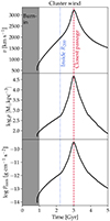 |
Fig. 1. Our magnetohydrodynamical wind tunnel simulation uses a time-dependent wind mimicking what a jellyfish galaxy experiences while orbiting a 1.1 × 10¹⁵ M⊙ cluster. This figure shows the resulting ICM wind speed, ICM wind density, and ram-pressure. In the first 1 Gyr we have a ‘burn-in phase’, where the galaxy settles into an equilibrium. Shortly after 2.0 Gyr the galaxy crosses R200 of the cluster, and 3.0 Gyr marks the closest passage to the centre, where the ram-pressure peaks. |
We used a turbulent time-dependent magnetic field in the wind with a thermal-to-magnetic pressure ratio of 50. The ICM wind and CGM were initialised with a third of solar metallicity, and the ISM itself was initialised with solar metallicity. We used solar abundances.
The ram-pressure stripping condition from Gunn et al. (1972) and Mo et al. (2010) reads
 (1)
(1)
As a result, the ISM of jellyfish galaxies are ‘outside-in stripped’ because the right-hand side of this equation is a declining function of radius. This of course assumes that the surface density profiles do not evolve in time. One source of clumps in the tail is hence expected to be stripped ISM gas, if the ram-pressure exceeds the criterion in Eq. (1). The functional forms of our stellar and gas surface density (Σ⋆, disc and Σgas, disc, respectively) can be found in Sparre et al. (2024). There, we even find that the inner parts of the disc at radii smaller than the scale radius are stripped during the central passage in the cluster.
2.2. Galaxy formation physics
We used the Auriga model of galaxy formation (Grand et al. 2017) but with the two main differences that we did not use active galactic nucleus feedback, and we used a fixed wind velocity, which is only realistic for a Milky Way-mass galaxy. We used the ISM model from Springel & Hernquist (2003), where gas cells with a density higher than the number density threshold for star formation (nsf = 0.157 cm−3) are multi-phase and have a contribution from a cold and a hot phase. Stellar population particles were probabilistically spawned from the star-forming cells, and stellar winds were released according to stellar evolution models (see Vogelsberger et al. 2013 for details).
2.3. Post-processing: Ionisation modelling
We used the CLOUDY (Ferland et al. 1998, 2017) tables presented in Hani et al. (2018) to calculate the H I content of our gas cells. We took into account a uniform UV background (from Faucher-Giguère et al. 2009), radiative cooling, self-shielding, and collisional ionisation.
As mentioned in Sect. 2.2, our ISM model treats star-forming gas cells as having a subgrid contribution from cold and hot phases. In our post-processing analysis, we set the temperature of star-forming gas cells to 103 K. Our results are not sensitive to this value since our main purpose is to ensure that the star-forming gas is included in the ISM according to the criterion in Sect. 2.4. An identical approach is often used in the literature, for example, in Ramesh et al. (2023).
2.4. Our definitions of ISM, CGM, and ICM
Here, we turn to the task of selecting gas residing in the ISM, CGM, and ICM. We based our definition on a combination of the thermal properties and the spatial location of a gas cell. We defined the centre of the galaxy (xgalaxy, ygalaxy, zgalaxy) to be the location of the most bound particle or cell in the simulation. As a measure of the radial extent of the gas of the H I disc (RHI), we determined the distance from the galaxy centre to the upstream location where the disc drops below a characteristic HI column density of 1020.5 cm−2 (column density maps and profiles in Appendix B motivate this choice). At times earlier than 2.60 Gyr, HI clouds are abundant in the CGM upstream of the galaxy. In order not to bias our disc estimates, we modelled the average column density profile with a parabola and performed a fit to determine RHI. At later times, the HI clouds in the CGM upstream of the galaxy centre are stripped, and the HI column density monotonically increases towards the galaxy centre. Thus, we can simply identify the extent of the HI disc by determining the point furthest upstream with a column density above 1020.5 cm−2. We further demonstrate and validate our methods for determining RHI in Appendix B.
To characterise gas in different phases, we used the following definitions of the ISM, CGM, and ICM gas reservoirs:
ISM: Gas with T ≤ 104.5 K and no more than 1.1RHI downstream from the galaxy centre (y ≤ ygalaxy + 1.1RHI). We multiplied RHI by a factor of 1.1 to bias our selection towards being inclusive when defining gas in the ISM. The spatial requirement ensures that the ISM belongs to the disc and not to clumps in the jellyfish tail far downstream from the galaxy.
ICM: Gas with log(T/K)≥0.2log[ρ/(M⊙ kpc−3)] + 5.8. This density dependent temperature cut is successful in isolating the thermal properties of our simulation’s injection region (the ICM) from the CGM.
CGM: Everything else.
In Appendix A, we illustrate the motivation for these selections by analysing the density-temperature diagram.
During infall, the stripping radius, which we identify with the smallest radius where the inequality in Eq. (1) is valid, is smaller in comparison to 1.1RHI. This is consistent with the jellyfish galaxy’s ISM experiencing ram-pressure stripping at these times. The stripping radius shrinks from 5.9 kpc (as the galaxy enters the cluster and passes through R200) to 1.0 kpc (which is reached at the centre of the cluster). In the same time interval, 1.1RHI shrinks from 33.0 kpc to 8.0 kpc.
2.5. Post-processing: friends-of-friends clump finding
We used a friends-of-friends (FoF) algorithm to find groups of gas cells with an H I number density larger than 0.01 cm−3 that are at a distance larger than 1.1RHI downstream from the galaxy centre. The density threshold of 0.01 cm−3 corresponds to an FoF linking length of 0.62 kpc (calculated as described in Sect. 3.4 of Sparre et al. 2024), and we required a minimum of ten cells in an FoF group. We used a serial python code as described further in Sparre et al. (2024). We refer to the identified ‘FoF groups’ as either ‘tail clumps’ or simply ‘clumps’ throughout this paper.
2.6. Tracing of gas
To track the Lagrangian path of gas mass, we used Monte Carlo tracer particles (Genel et al. 2013). At t = 0, we created five tracers within each gas cell. During the simulation, tracer particles were transferred between gas cells, stellar population particles, and wind particles such that an ensemble of tracers enabled us to follow the Lagrangian gas flows in a statistical fashion. The use of tracer particles (instead of directly following the paths of gas cells) is correct and preferred since mass transfer occurs between different gas cells.
We first focused our tracer analysis at a time of 2.50 Gyr. We used our FoF algorithm to identify H I clumps in the tail downstream from the jellyfish galaxy. For each tail clump, we selected all the tracer particles and tracked their density, temperature, and spatial coordinates back in time. Based on their properties at t = 1 Gyr, we determined their origin to be the ISM, CGM, or ICM. This time was chosen because it corresponds to the time when the ‘burn-in phase’ finishes and the galaxy is in quasi-equilibrium. We use the notation CGM → clumps to refer to gas tracers that started out in the CGM at t = 1 Gyr and reside in tail clumps at t = 2.50 Gyr. We use a similar notation for tracers starting in the ISM and ending up in tail clumps (see Table 1).
Origin and evolutionary paths of gas ending up in clumps in the galaxy tail traced using Monte Carlo tracers.
For the ICM, we introduce the tag ‘ICM → clumps’. It is given to tracers that meet one of the following two criteria. (1) At t = 1 Gyr they had a density and temperature obeying our ICM criterion. Or (2) at a time of 1.0 ≤ t/Gyr ≤ 2.50 resided in the injection region of the simulation wind tunnel.
For the tracers characterised as ‘CGM → clumps’, we define a subset of tracers that have had an in-between phase residing in the disc’s ISM. We refer to these tracers as CGM → ISM → clumps. Similarly, we introduce the notation ICM → ISM → clumps for ICM tracers that have been accreted onto the ISM before ending up in the galaxy tail.
If we let f denote the fractional contribution to the H I mass in a clump, we can calculate the fraction of gas that has resided in the ISM at some point prior to a time of 2.50 Gyr as
 (2)
(2)
This quantity plays a key role in our analysis of gas flows. In this subsection, we have explained how our tracer analysis was used to characterise gas at a snapshot of 2.50 Gyr. We repeated this process at times of 2.75 and 3.25 Gyr, and we present our results in the next section.
3. Results
3.1. Validating the thermal profiles with state-of-the-art cosmological simulations
Before analysing the role of CGM gas in the build-up of the jellyfish tail, we validate the initial CGM of the jellyfish galaxy. To do this we analysed our simulation after the burn-in phase at 1.0 Gyr and at 2.0 Gyr, when the galaxy enters R200 of the cluster. In this validation, we compare our CGM profiles to five galaxies from the cosmological Auriga simulations (Grand et al. 2017) of Milky Way-mass galaxies at a redshift of z = 0.
In Fig. 2, we plot the thermal profiles calculated in spherical shells equally spaced in logarithmic radius (logr). For r ≳ 100 kpc, our galaxy is significantly hotter than the Auriga simulations. The reason is the hot ICM wind. Except for this physically desired effect, we find quantitatively good agreement between our simulation and Auriga, implying that we have a CGM consistent with state-of-the-art cosmological simulations of Milky Way-mass galaxies. Our initial conditions are hence ideal for studying how ram-pressure stripping affects the CGM.
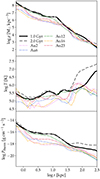 |
Fig. 2. Density, temperature, and thermal pressure as a function of radius for our simulated jellyfish galaxy at 1.0 and 2.0 Gyr. We compare our simulated profiles at 1.0 and 2.0 Gyr to the redshift z = 0 profiles of five different simulations from the Auriga suite. We note that the increase of temperature and thermal pressure at the largest radii delineates the transition from the CGM to the hot ICM wind. Hence, there is good agreement between our simulation and Auriga, implying that our adopted CGM is consistent with cosmological simulations. |
The galaxy experiences an ICM density of 102.7 M⊙ kpc−3 as it enters R200 and a peak of 104.7 M⊙ kpc−3 at the time of the nearest passage of the cluster centre (see Fig. 1). The CGM, on the other hand (see radii ranging from ∼101.5 kpc to 102 kpc in Fig. 2), spans densities ranging from 104 to 105 M⊙ kpc−3. Around the time of the infall, the CGM is hence in the cloud-crushing regime (ρCGM > ρICM), as identified by Ghosh et al. (2024), and closer to the nearest passage there would co-exist zones in the cloud-crushing- and bubble-regimes (the latter regime is defined as ρCGM < ρICM) – which is a realistic scenario, as discussed in Sect. 5.2.1 of Ghosh et al. (2024).
3.2. The origin of gas in the tail
In this section, we turn to the key question of this paper and analyse the tail of the jellyfish galaxy. We present the analysis for three different times: 2.50, 2.75, and 3.25 Gyr. The first two times sample the infall of the galaxy onto the galaxy cluster before the central passage, and the third is after the central passage.
In Fig. 3, we plot the H I column density (upper row) in order to present a visualisation of the cold gas in the tail in the wake of the galaxy, which points in the direction of the ICM velocity (and which is also found in the cosmological simulations of Yun et al. 2019). For the tail clumps identified at each snapshot, we show the mass fraction of the origin of the cold gas (ISM → clumps, CGM → clumps, or ICM → clumps) in the second row. The mass fraction of the gas that at some point has been a part of the cold ISM according to Eq. (2) is shown in the third row, together with the sub-classes outlined in Table 1. The mass-weighted y-velocity for each clump relative to the stars in the galaxy, that is vy − ⟨vy⋆⟩, is shown in the fourth row. We note that the velocity of the ICM wind relative to the galaxy (vwind − ⟨vy⋆⟩) is 2211, 2591, and 2771 km s−1 at the times of 2.50, 2.75, and 3.25 Gyr, respectively. Hence, the tail clumps are not sufficiently accelerated to be co-moving with the wind.
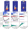 |
Fig. 3. H I column density (upper panels); mass fraction of tail clumps initially residing in the ISM, CGM, or ICM (second row); mass fraction of different paths through the ISM from Table 1 (third row); and the mass-weighted vy-velocity of each tail clump (lower panels) for three times (2.50, 2.75, and 3.25 Gyr). We note that the central passage took place between the second and third analysed time. The white contours indicate the surface density of stars. The yellow arrow marks the y-value, which divides the tail from the galactic disc (ygalaxy + 1.1RHI). The majority of the mass in the tail clumps initially resided in the CGM for these three snapshots. Well before the central passage (at 2.50 Gyr), the dominant mass fraction of the tail’s H I clumps were accreted directly from the CGM. After the central passage (at 3.25 Gyr), about half of the gas in the tail initially resided in the CGM, but it was almost exclusively accreted onto the ISM before being stripped and finally assembled in the jellyfish tail. The other half of the gas originates in the initial ISM that was already present at t = 1 Gyr. |
We observed a remarkable H I tail present at all three times with a clumpy structure characteristic of shattering, similar to what we concluded in Sparre et al. (2024). The downstream clumps are dominated by gas that initially resided in the CGM, especially at t = 2.50 and 2.75 Gyr. There are two reasons for this. First, a fraction of the CGM gas is directly pushed by ICM ram pressure into the tail without ever entering the disc’s ISM. This can, for example, be seen ≳200 kpc downstream at 2.75 Gyr, where f(CGM → clumps) is significantly larger than f(through ISM). Secondly, the gas in our simulated galaxy (and galaxies in general; see Suresh et al. 2019) is continuously being transferred between the CGM and ISM. This highlights the result that it is necessary to include a realistic CGM in idealised jellyfish galaxy simulations to reliably study the structure of the tail.
Next, we further assess the fraction of gas, f(through ISM), that at some point during the simulation was accreted onto the disc’s ISM before entering the shattered tail. There is a transition occurring, when comparing the times before (2.50 and 2.75 Gyr) and after (3.25 Gyr) the central passage. At the latter time, a clear majority of the gas in the shattered tail has resided in the ISM at some point during the simulation, while at the same time about 50% of this gas originated in the CGM (i.e. the channel CGM → ISM → clumps slightly dominates). At the two earlier times, a lower fraction of gas (in comparison to 3.25 Gyr) resided in the ISM before entering the tail. Thus, during the galaxy’s infall, there is a larger fraction of gas that has never been part of the ISM. This gas has been mixed with the stripped cold ISM to an intermediate temperature that is thermally unstable so that it loses its thermal energy via radiative cooling before entering the cold phase in the tail and shatters into smaller cloudlets.
The majority of the cold gas in the tail originates in the CGM, which is less dense and hence much easier to accelerate by the wind in comparison to the denser ISM. Hence, this explains the enormous extent of some jellyfish tails. Mixing in the hot ICM and cooling it to 104 K further adds momentum to the tails (in the galaxy rest frame), but this phase is small by mass in comparison to the other two phases.
This transition is also visible in the H I projections. At 3.25 Gyr, the clumps in the tail are elongated, which is a consequence of these clumps having been directly stripped from the ISM, in accordance with the classic picture of ram-pressure stripping (Gunn et al. 1972). At earlier times, however, the clumps are less elongated and ‘more shattered’ (following the nomenclature of McCourt et al. 2018), so here thermal instability and radiative cooling of CGM gas, which has never resided in the ISM, is more important.
The finding that the ‘through-ISM-channel’ completely dominates after the time of the nearest cluster passage is of course a result of the ram-pressure stripping history. To some degree, this is a coincidence of the choice of our adopted galaxy orbit that implies that this transition occur at around the closest passage.
The monotonically increasing trend in vy versus y − ygalaxy shows that clumps are accelerated as they move downstream. Such a trend is expected during the infall in the cluster. We observed that the tail gas moves faster downstream after the central passage in comparison to before. So after the passage, we not only observed a transition in the origin of the gas but also in the tail velocity.
The above results are insensitive to the choice of FoF parameters. We varied the minimum number of cells that constitute a clump between five, ten (our standard choice), and 20. We also ran the analysis with a ten times high FoF density threshold in comparison to our standard value (0.01 cm−2). These variations of course changed the total number of FoF groups and their masses, but they did not change the overall findings and scalings of the curves in Fig. 3.
Using our intermediate resolution simulations from Sparre et al. (2024), we also checked how our Fig. 3 would change if the angle between the ICM wind and the galaxy’s rotation axis would change from 60° (as in the simulation presented in this paper) to 0, 30, and 90°. Our most important results, which is that f(through ISM) increases for the tail later in the simulation, is independent of this angle. That being said, the experienced ram pressure is of course inclination dependent, as we also discuss in Sparre et al. (2024).
3.3. The baryonic mass budget
In Fig. 4, we assess the build-up of the tail from a mass budget perspective. We focus on the cold gas mass with a temperature below 104.5 K. We plot the (1) total cold gas mass in the simulation, (2) the cold gas mass in the tail, (3) the cold gas mass associated with the galaxy, and (4) the stars formed after t = 2 Gyr, which is when the galaxy started to experience an appreciable ram pressure. The mass of cold gas in the galactic disc significantly declines from the entrance of R200 until the central passage in the cluster. This is an effect of ram-pressure stripping as well as stars forming during the infall (also shown in the figure). Conversely, the mass of cold gas in the tail grows by a factor of three from the infall to the central passage. This is expected from idealised simulations of cloud-wind interactions in the ‘growth’ regime of large clouds (e.g. Armillotta et al. 2017; Gronke & Oh 2018; Sparre et al. 2020; Li et al. 2020). Furthermore, continued star formation and enhanced ram-pressure stripping of the ISM during and after the central passage causes the amount of cold gas to decline in the disc and tail. We note that the formation of stars at late times is consistent with the finding from Rohr et al. (2023) that the jellyfish galaxies continue forming stars until they have lost approximately 98% of their gas. Overall, the evolution of the gas shows the evolution from a gas-rich spiral galaxy to a less star-forming, gas-poor galaxy during the first infall onto the cluster. This is also consistent with Rohr et al. (2023), who find that ram-pressure stripping is capable of stripping jellyfish galaxies from z = 0.5 to z = 0.
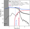 |
Fig. 4. Time evolution of the (1) total cold gas mass (defined as T ≤ 104.5 K) in the simulation, (2) the cold gas in the tail, (3) the cold gas associated with the galactic disc, and (4) the total mass of stars formed since t = 2 Gyr. As expected from idealised simulations of cloud-wind interactions in the regime of large clouds, the cold gas mass of the tail increases after entering the cluster until a time close to the closest central passage. Continued star formation and enhanced ram-pressure stripping of the ISM during the central passage causes a drop of the cold gas in the disc and tail. |
3.4. The metallicity in the gaseous tail
The physics of jellyfish tails can be constrained by, for example, radio observations (Müller et al. 2021; Roberts et al. 2021; Ignesti et al. 2022), but a promising observable is also the gas metallicity of the clumps. Franchetto et al. (2021) has shown that the gas metallicity in the tail is influenced by the mixing of gas from the ICM wind and the galaxy. Here, we study this connection further.
We remind the reader that we initialised gas in the ISM with solar metallicity, ZISM = Z⊙, and gas in the CGM and ICM was initialised with a three-times lower metallicity, ZCGM, ICM = Z⊙/3. In Fig. 5 (left panel), we show the gas metallicity of tail clumps as a function of f(through ISM). During the infall in the cluster (at 2.50 and 2.75 Gyr), there is a strong correlation, which is expected because an over-abundance of metals is initialised and produced in the galactic ISM. After infall (at 3.25 Gyr), the majority of the gas in the tail clumps has resided in the ISM at some point during the simulation. In the meanwhile, the ISM has been significantly enriched during the simulation time so that the tail is not only characterised by a larger metallicity in comparison to earlier times but also has super-solar metallicities.
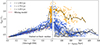 |
Fig. 5. Gas metallicity of the clumps in the tail. The clumps are shown as different symbols denoting the different analysis times. Left panel: Gas metallicity as a function of the mass fraction of gas that at some point during the simulation has resided in the jellyfish galaxy’s ISM. During infall (2.50 and 2.75 Gyr), there is a correlation between these two quantities. This indicates that the metallicity of the jellyfish tail is influenced by mixing of high-metallicity ISM gas with low-metallicity gas from the CGM and ICM. We quantified this with a ‘mixing model’, |
We adopted a simple model for the jellyfish tail metallicity:
 (3)
(3)
Specified to our simulations, this model assumes that all gas that ever was in the galactic ISM has solar metallicity and everything else has one-third solar, so it assumes that the ISM metallicity is not evolving. This toy model has the implicit assumption that the inflow of low-metallicity gas into the ISM and the outflow rate of enriched gas are balanced by metals produced by star formation. We refer to this as a ‘mixing model’.
This model correctly predicts an increasing metallicity as a function of f(through ISM) – observed at times 2.50 and 2.75 Gyr – and delineates the lower envelope of the relation. This is expected because the model does not account for additional enrichment due to ongoing star formation and stellar mass return and indicates that mixing of ISM and CGM gas can explain the metallicity of our tail clumps. At a time of 3.25 Gyr, the ISM has been significantly enriched, so at this point the model no longer gives an accurate description.
In the right panel of Fig. 5, we show the gas metallicity as a function of the downstream distance from the galaxy. At all times, we see a declining metallicity as a function of distance. At t = 2.50 and 2.75 Gyr, the metallicity is higher in the immediate tail at y − ygalaxy ≲ 80 kpc in comparison to further downstream, and at t = 3.25 Gyr, we observed a more prevalent monotonically declining trend reaching further downstream from the galaxy. We thus overall confirm the declining metallicity in the tail as seen in Franchetto et al. (2021) and in the recent modelling of Ghosh et al. 2024 (see their Sect. 4.1.3).
4. Discussion on ISM and CGM stripping
The CGM becomes completely stripped in our simulation. This can be seen by comparing our Fig. B.1 and Fig. B.2, which show the HI column density at a time of 2 Gyr and 2.75 Gyr, respectively. At the latter time, there is a complete lack of > 1019 cm−2 gas upstream from the disc. On a similar note, a short stripping timescale of CGM gas was found in satellites orbiting a MW-like halo in Zhu et al. (2024), who found a CGM stripping timescale of a few hundred million years. We note that we have a peak ram pressure of approximately 3 × 10⁻¹⁰ g cm−1 s−2, which is three orders of magnitudes larger than Zhu et al. (2024) (3.94 × 10⁻¹³ g cm−1 s−2), but the authors also simulated a less massive system, which explains the similarly short stripping timescales. Zhu et al. (2024) also found a large fraction of the ISM survives the ram-pressure stripping, similar to us (see Fig. 2 of Sparre et al. 2024).
Roy et al. (2024) performed a similar analysis of ISM stripping timescales in simulations of satellites orbiting a MW-like galaxy. They found ISM stripping timescales of 0.25 to 3–4 Gyr, depending on the satellite’s mass. The ISM of their most-massive satellite was continuously fed by gas being accreted from the host Milky Way-mass halo’s reservoir. Although we did not see gas being accreted from the ICM to the ISM as a dominant channel, we found a similar result that ram-pressure stripping in our simulations is not capable of fully removing the ISM of the jellyfish galaxy.
In this paper, we have not attempted to resolve the star-forming clouds or the ISM, and instead we have imposed the star formation law from Springel & Hernquist (2003). The ISM-associated observables are therefore not necessarily correctly predicted, and we leave it to future work to carry out simulations with a resolved ISM model and to predict the above-mentioned observables. Expanding our simulation setup to a more structured ISM modelling for a jellyfish galaxy orbiting a galaxy cluster will likely reveal the impact of the existence of these two tail formation mechanisms, and it may even lead to an evolutionary sequence for jellyfish galaxies and their tails. A natural follow-up question is also how the signatures of the two mechanisms are imprinted into the common jellyfish observables, such as maps of UV intensity, emission lines, X-ray, radio and molecular gas.
Another advantage of using a structured ISM model is associated with the mixing layer, which has a temperature in between the stripped cool gas and the hot gas (Tonnesen & Bryan 2021; Roy et al. 2024). This cooling may induce formation of condensed clouds (Gronke & Oh 2018; Abruzzo et al. 2023). For this to happen, it is of course necessary to fully capture the density and temperature gradients of the gas in the mixing layer surrounding the cold gas. A potential caveat here comes from the treatment of the ISM in our physics model. When gas is denser than the star formation threshold, it is described by an effective equation of state, and stellar winds are probabilistically ejected from the gas cells. The stellar wind particles are decoupled from the hydrodynamical interactions until they are outside the star-forming region. Because of this behaviour, we do not expect the detailed structure of the star-forming gas or the layers surrounding them to be fully realistic in our current simulations. Re-running with a structured ISM model that models galactic winds emerging from a combination of supernova, cosmic ray, and radiative energy injection would improve the modelling of the mixing layers and the ISM structure (Thomas et al. 2024).
5. Conclusion
This paper has revealed two distinct formation mechanisms of the tails of jellyfish galaxies. In one scenario, when ram-pressure is not sufficiently strong to strip the majority of the ISM, tails are formed by CGM gas that is being transferred into the tail, where it mixes with the stripped ISM to intermediate temperatures. The mixed gas is subject to thermal instability such that the ensuing fast radiative cooling causes the formation of multi-phase tails. However, when the ram pressure from the ICM is strong enough, the ISM is directly stripped and moved into the wake of the galaxy, where a dense tail is formed. This mechanism follows the idea of the analytical model of Gunn et al. (1972). These two formation mechanisms are clearly identified in our numerical simulation, but it is still an open question as to whether and how these processes can be identified in observations.
A very recent publication by Ghosh et al. (2024) also identifies the importance of including the CGM when studying the stripping of jellyfish galaxies and the build-up of their tails. In comparison to our work, they performed a comprehensive study of stripping regimes in multiple simulations, where they identify the ‘bubble-mode’ and ‘cloud-crushing-regime’ for CGM stripping. The strategy of our paper is to include a time-varying wind in a single simulation and to also include radiative cooling processes, star formation, and chemical enrichment. This approach enabled us to study, for example, the metallicity evolution and shattering of tail clumps. We find it encouraging that both studies identify the CGM as playing a key role in forming jellyfish tails.
Acknowledgments
We acknowledge support by the European Research Council under ERC-AdG grant PICOGAL-101019746.
References
- Abruzzo, M. W., Bryan, G. L., & Fielding, D. B. 2022, ApJ, 925, 199 [NASA ADS] [CrossRef] [Google Scholar]
- Abruzzo, M. W., Fielding, D. B., & Bryan, G. L. 2023, ApJ, submitted [arXiv:2307.03228] [Google Scholar]
- Anglés-Alcázar, D., Faucher-Giguère, C.-A., Kereš, D., et al. 2017, MNRAS, 470, 4698 [CrossRef] [Google Scholar]
- Armillotta, L., Fraternali, F., Werk, J. K., Prochaska, J. X., & Marinacci, F. 2017, MNRAS, 470, 114 [NASA ADS] [CrossRef] [Google Scholar]
- Bekki, K. 2009, MNRAS, 399, 2221 [Google Scholar]
- Bekki, K., & Couch, W. J. 2003, ApJ, 596, L13 [NASA ADS] [CrossRef] [Google Scholar]
- Boselli, A., Fossati, M., & Sun, M. 2022, A&ARv, 30, 3 [NASA ADS] [CrossRef] [Google Scholar]
- Butcher, H., & Oemler, A. 1984, J., ApJ, 285, 426 [NASA ADS] [Google Scholar]
- Dressler, A. 1980, ApJ, 236, 351 [Google Scholar]
- Durret, F., Chiche, S., Lobo, C., & Jauzac, M. 2021, A&A, 648, A63 [NASA ADS] [CrossRef] [EDP Sciences] [Google Scholar]
- Dursi, L. J., & Pfrommer, C. 2008, ApJ, 677, 993 [NASA ADS] [CrossRef] [Google Scholar]
- Faucher-Giguère, C.-A., Lidz, A., Zaldarriaga, M., & Hernquist, L. 2009, ApJ, 703, 1416 [Google Scholar]
- Ferland, G. J., Korista, K. T., Verner, D. A., et al. 1998, PASP, 110, 761 [Google Scholar]
- Ferland, G. J., Chatzikos, M., Guzmán, F., et al. 2017, Rev. Mex. Astron. Astrofis., 53, 385 [NASA ADS] [Google Scholar]
- Franchetto, A., Tonnesen, S., Poggianti, B. M., et al. 2021, ApJ, 922, L6 [NASA ADS] [CrossRef] [Google Scholar]
- Genel, S., Vogelsberger, M., Nelson, D., et al. 2013, MNRAS, 435, 1426 [NASA ADS] [CrossRef] [Google Scholar]
- Ghosh, R., Dutta, A., & Sharma, P. 2024, MNRAS, 531, 3445 [NASA ADS] [CrossRef] [Google Scholar]
- Girichidis, P., Naab, T., Walch, S., & Berlok, T. 2021, MNRAS, 505, 1083 [NASA ADS] [CrossRef] [Google Scholar]
- Grand, R. J. J., Gómez, F. A., Marinacci, F., et al. 2017, MNRAS, 467, 179 [NASA ADS] [Google Scholar]
- Gronke, M., & Oh, S. P. 2018, MNRAS, 480, L111 [Google Scholar]
- Gunn, J. E., Gott, J., & Richard, I. 1972, ApJ, 176, 1 [Google Scholar]
- Hani, M. H., Sparre, M., Ellison, S. L., Torrey, P., & Vogelsberger, M. 2018, MNRAS, 475, 1160 [CrossRef] [Google Scholar]
- Hernquist, L. 1990, ApJ, 356, 359 [Google Scholar]
- Ignesti, A., Vulcani, B., Poggianti, B. M., et al. 2022, ApJ, 924, 64 [NASA ADS] [CrossRef] [Google Scholar]
- Kanjilal, V., Dutta, A., & Sharma, P. 2021, MNRAS, 501, 1143 [Google Scholar]
- Krogager, J. K., Møller, P., Fynbo, J. P. U., & Noterdaeme, P. 2017, MNRAS, 469, 2959 [NASA ADS] [CrossRef] [Google Scholar]
- Lee, J., Kimm, T., Katz, H., et al. 2020, ApJ, 905, 31 [NASA ADS] [CrossRef] [Google Scholar]
- Lee, J., Kimm, T., Blaizot, J., et al. 2022, ApJ, 928, 144 [NASA ADS] [CrossRef] [Google Scholar]
- Li, Z., Hopkins, P. F., Squire, J., & Hummels, C. 2020, MNRAS, 492, 1841 [NASA ADS] [CrossRef] [Google Scholar]
- McCourt, M., Oh, S. P., O’Leary, R., & Madigan, A.-M. 2018, MNRAS, 473, 5407 [Google Scholar]
- Mo, H., van den Bosch, F. C., & White, S. 2010, Galaxy Formation and Evolution (Cambridge University Press) [Google Scholar]
- Moore, B., Katz, N., Lake, G., Dressler, A., & Oemler, A. 1996, Nature, 379, 613 [Google Scholar]
- Müller, A., Poggianti, B. M., Pfrommer, C., et al. 2021, Nat. Astron., 5, 159 [Google Scholar]
- Owen, F. N., Keel, W. C., Wang, Q. D., Ledlow, M. J., & Morrison, G. E. 2006, AJ, 131, 1974 [Google Scholar]
- Péroux, C., & Howk, J. C. 2020, ARA&A, 58, 363 [CrossRef] [Google Scholar]
- Pfrommer, C., & Dursi, L. J. 2010, Nat. Phys., 6, 520 [NASA ADS] [CrossRef] [Google Scholar]
- Poggianti, B. M., Fasano, G., Omizzolo, A., et al. 2016, AJ, 151, 78 [Google Scholar]
- Poggianti, B. M., Moretti, A., Gullieuszik, M., et al. 2017, ApJ, 844, 48 [Google Scholar]
- Poggianti, B. M., Ignesti, A., Gitti, M., et al. 2019, ApJ, 887, 155 [Google Scholar]
- Prochaska, J. X., Werk, J. K., Worseck, G., et al. 2017, ApJ, 837, 169 [CrossRef] [Google Scholar]
- Quilis, V., Moore, B., & Bower, R. 2000, Science, 288, 1617 [Google Scholar]
- Ramatsoku, M., Serra, P., Poggianti, B. M., et al. 2019, MNRAS, 487, 4580 [Google Scholar]
- Ramesh, R., Nelson, D., & Pillepich, A. 2023, MNRAS, 518, 5754 [Google Scholar]
- Richter, P., Nuza, S. E., Fox, A. J., et al. 2017, A&A, 607, A48 [NASA ADS] [CrossRef] [EDP Sciences] [Google Scholar]
- Roberts, I. D., van Weeren, R. J., McGee, S. L., et al. 2021, A&A, 650, A111 [NASA ADS] [CrossRef] [EDP Sciences] [Google Scholar]
- Roediger, E., & Hensler, G. 2005, A&A, 433, 875 [NASA ADS] [CrossRef] [EDP Sciences] [Google Scholar]
- Rohr, E., Pillepich, A., Nelson, D., et al. 2023, MNRAS, 524, 3502 [NASA ADS] [CrossRef] [Google Scholar]
- Roman-Oliveira, F. V., Chies-Santos, A. L., Rodríguez del Pino, B., et al. 2019, MNRAS, 484, 892 [Google Scholar]
- Roy, M., Su, K.-Y., Tonnesen, S., Fielding, D. B., & Faucher-Giguère, C.-A. 2024, MNRAS, 527, 265 [Google Scholar]
- Ruszkowski, M., Brüggen, M., Lee, D., & Shin, M. S. 2014, ApJ, 784, 75 [NASA ADS] [CrossRef] [Google Scholar]
- Schneider, E. E., & Robertson, B. E. 2017, ApJ, 834, 144 [NASA ADS] [CrossRef] [Google Scholar]
- Schneider, E. E., Robertson, B. E., & Thompson, T. A. 2018, ApJ, 862, 56 [NASA ADS] [CrossRef] [Google Scholar]
- Schulz, S., & Struck, C. 2001, MNRAS, 328, 185 [NASA ADS] [CrossRef] [Google Scholar]
- Smith, R. J., Lucey, J. R., Hammer, D., et al. 2010, MNRAS, 408, 1417 [Google Scholar]
- Sparre, M., Pfrommer, C., & Vogelsberger, M. 2019, MNRAS, 482, 5401 [Google Scholar]
- Sparre, M., Pfrommer, C., & Ehlert, K. 2020, MNRAS, 499, 4261 [NASA ADS] [CrossRef] [Google Scholar]
- Sparre, M., Pfrommer, C., & Puchwein, E. 2024, MNRAS, 527, 5829 [Google Scholar]
- Springel, V., & Hernquist, L. 2003, MNRAS, 339, 289 [Google Scholar]
- Springel, V., Di Matteo, T., & Hernquist, L. 2005, MNRAS, 361, 776 [Google Scholar]
- Steinhauser, D., Schindler, S., & Springel, V. 2016, A&A, 591, A51 [NASA ADS] [CrossRef] [EDP Sciences] [Google Scholar]
- Sun, M., Donahue, M., & Voit, G. M. 2007, ApJ, 671, 190 [Google Scholar]
- Suresh, J., Nelson, D., Genel, S., Rubin, K. H. R., & Hernquist, L. 2019, MNRAS, 483, 4040 [NASA ADS] [CrossRef] [Google Scholar]
- Thomas, T., Pfrommer, C., & Pakmor, R. 2024, A&A, submitted [arXiv:2405.13121] [Google Scholar]
- Tonnesen, S. 2019, ApJ, 874, 161 [Google Scholar]
- Tonnesen, S., & Bryan, G. L. 2009, ApJ, 694, 789 [NASA ADS] [CrossRef] [Google Scholar]
- Tonnesen, S., & Bryan, G. L. 2012, MNRAS, 422, 1609 [CrossRef] [Google Scholar]
- Tonnesen, S., & Bryan, G. L. 2021, ApJ, 911, 68 [NASA ADS] [CrossRef] [Google Scholar]
- Tumlinson, J., Peeples, M. S., & Werk, J. K. 2017, ARA&A, 55, 389 [Google Scholar]
- van de Voort, F., Springel, V., Mandelker, N., van den Bosch, F. C., & Pakmor, R. 2019, MNRAS, 482, L85 [NASA ADS] [CrossRef] [Google Scholar]
- Vogelsberger, M., Genel, S., Sijacki, D., et al. 2013, MNRAS, 436, 3031 [Google Scholar]
- Werk, J. K., Prochaska, J. X., Thom, C., et al. 2013, ApJS, 204, 17 [NASA ADS] [CrossRef] [Google Scholar]
- Werk, J. K., Prochaska, J. X., Cantalupo, S., et al. 2016, ApJ, 833, 54 [NASA ADS] [CrossRef] [Google Scholar]
- Yagi, M., Yoshida, M., Komiyama, Y., et al. 2010, AJ, 140, 1814 [Google Scholar]
- Yoshida, M., Yagi, M., Komiyama, Y., et al. 2008, ApJ, 688, 918 [Google Scholar]
- Yun, K., Pillepich, A., Zinger, E., et al. 2019, MNRAS, 483, 1042 [Google Scholar]
- Zhu, J., Tonnesen, S., Bryan, G. L., & Putman, M. E. 2024, ApJ, 974, 142 [NASA ADS] [CrossRef] [Google Scholar]
Appendix A: Defining the ISM, CGM, and ICM gas reservoirs
We now describe our choices of the ISM, CGM, and ICM definition from Sect. 2.4 in detail. With these definitions the (ρ, T)-plane is used to divide up the phases, according to the dashed lines in Fig. A.1. We have adopted an ISM definition aimed at including cold gas in the disc. We have adopted a definition of ICM gas selecting all gas in the wind injection region during the simulation. Finally the CGM is defined to be gas which is neither ISM or ICM – this requirement effectively selects halo gas colder or comparable to the virial temperature. Our definitions are explicitly stated in Sect. 2.4.
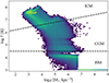 |
Fig. A.1. Tracer classification based on the (ρ, T)-plane. The background histogram shows the gas cells at a time of 2.50 Gyr, and the dashed lines divide our definitions of ISM, CGM, and ICM. In Sect. 2.4 we show quantitative definitions of these reservoirs. |
Appendix B: Determination of the HI disc radius
We now introduce and define the HI disc radius (RHI), which we use in Sect. 2 to define the tail of the jellyfish galaxy. Conceptually, we would like to determine it as the radius, where the HI column density of the disc reaches the value typically associated with a galaxy’s ISM (≈1020.5–1022 cm−2, see table 5 and fig. 8 of Krogager et al. 2017).
We determine the projected HI column density in the (x, y)-plane using a 100 × 200 histogram grid distributed at x − xgalaxy = ±25 kpc and y − ygalaxy = ±50 kpc. For each of these grid cells, we calculate  numerically. The resulting projection plots at a time of 2.0 and 2.75 Gyr are shown in Fig. B.1 and B.2, respectively (left panels). Next we determine the characteristic HI value as a function of y, by averaging over x:
  . The right panels of Fig. B.1 and B.2 show this averaged profile.
By comparing the HI projection at 2.0 and 2.75 Gyr, we see that the former snapshot has a richer and more inhomogeneous gaseous structure upstream from the galaxy. This is a contribution from the ISM and CGM, which has not yet been stripped at 2.0 Gyr. To derive an extent of the HI disc, we here fit a second order polynomial of the form, log⟨NHI⟩=A(y − ygalaxy)2 + B(y − ygalaxy)+C. This fit is shown in the right panel of the figures. At 2.0 Gyr we use this fit to determine the y-value, where the disc HI column density reaches a value of 1020.5 cm−2.
At later times, for example, at 2.75 Gyr, the CGM upstream from the disc has been stripped. Instead of performing a fit, we simply take the first y-value with ⟨NHI⟩≥1020.5 cm−2. At t ≤ 2.60 Gyr we perform fits as described above, and at later times, we identify the lowest y-value with ⟨NHI⟩≥1020.5 cm−2. We visually inspect all snapshots of the simulations to check that this gives a reasonable behaviour of the HI disc radius. In the left panel of Fig. B.1 and B.2 we plot the fitted- and value-identified radius as a blue and black circle, respectively. The time evolution of our identified RHI is shown in Fig. B.3. We see that this quantity increases from the start of the simulation until the galaxy enters R200 in the galaxy cluster. This is because of gas accreted to the ISM from the CGM. As the ram-pressure increases the HI radius declines until the nearest passage. At later times, the HI radius slowly increases in our simulation. The resulting time-depending HI radius enables us to classify whether gas downstream from the galaxy centre belongs to the tail or the disc ISM (Sect. 2.4).
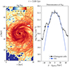 |
Fig. B.1. HI projected column density of the jellyfish galaxy (left panel), where the cross marks the galaxy centre, and the blue triangle and black circle mark RHI determined with a fit and by identifying the furthest upstream location with ⟨NHI⟩≥1020.5 cm−2, respectively. In the right panel, we plot ⟨NHI⟩ (see text for details) and mark RHI determined with the different methods. At this early time of t = 2.0 Gyr, there are CGM clumps upstream from the galaxy, so we use a fit to determine the RHI for the disc. |
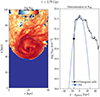 |
Fig. B.2. Same as Fig. B.1 but for a time of t = 2.75 Gyr, where we instead of fitting the averaged column density with a parabola simply determine the furthest upstream location with ⟨NHI⟩≥1020.5 cm−2 (see black triangle). This approach is sufficient and preferred at times, where HI clumps in the CGM upstream the galaxy are absent. |
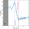 |
Fig. B.3. Evolution of the HI radius, which has been determined with a fit for t ≤ 2.60 Gyr, and a simple detection of the furthest upstream location with ⟨NHI⟩≥1020.5 cm−2 at later times. |
All Tables
Origin and evolutionary paths of gas ending up in clumps in the galaxy tail traced using Monte Carlo tracers.
All Figures
|
Fig. 1. Our magnetohydrodynamical wind tunnel simulation uses a time-dependent wind mimicking what a jellyfish galaxy experiences while orbiting a 1.1 × 10¹⁵ M⊙ cluster. This figure shows the resulting ICM wind speed, ICM wind density, and ram-pressure. In the first 1 Gyr we have a ‘burn-in phase’, where the galaxy settles into an equilibrium. Shortly after 2.0 Gyr the galaxy crosses R200 of the cluster, and 3.0 Gyr marks the closest passage to the centre, where the ram-pressure peaks. |
| In the text | |
|
Fig. 2. Density, temperature, and thermal pressure as a function of radius for our simulated jellyfish galaxy at 1.0 and 2.0 Gyr. We compare our simulated profiles at 1.0 and 2.0 Gyr to the redshift z = 0 profiles of five different simulations from the Auriga suite. We note that the increase of temperature and thermal pressure at the largest radii delineates the transition from the CGM to the hot ICM wind. Hence, there is good agreement between our simulation and Auriga, implying that our adopted CGM is consistent with cosmological simulations. |
| In the text | |
|
Fig. 3. H I column density (upper panels); mass fraction of tail clumps initially residing in the ISM, CGM, or ICM (second row); mass fraction of different paths through the ISM from Table 1 (third row); and the mass-weighted vy-velocity of each tail clump (lower panels) for three times (2.50, 2.75, and 3.25 Gyr). We note that the central passage took place between the second and third analysed time. The white contours indicate the surface density of stars. The yellow arrow marks the y-value, which divides the tail from the galactic disc (ygalaxy + 1.1RHI). The majority of the mass in the tail clumps initially resided in the CGM for these three snapshots. Well before the central passage (at 2.50 Gyr), the dominant mass fraction of the tail’s H I clumps were accreted directly from the CGM. After the central passage (at 3.25 Gyr), about half of the gas in the tail initially resided in the CGM, but it was almost exclusively accreted onto the ISM before being stripped and finally assembled in the jellyfish tail. The other half of the gas originates in the initial ISM that was already present at t = 1 Gyr. |
| In the text | |
|
Fig. 4. Time evolution of the (1) total cold gas mass (defined as T ≤ 104.5 K) in the simulation, (2) the cold gas in the tail, (3) the cold gas associated with the galactic disc, and (4) the total mass of stars formed since t = 2 Gyr. As expected from idealised simulations of cloud-wind interactions in the regime of large clouds, the cold gas mass of the tail increases after entering the cluster until a time close to the closest central passage. Continued star formation and enhanced ram-pressure stripping of the ISM during the central passage causes a drop of the cold gas in the disc and tail. |
| In the text | |
|
Fig. 5. Gas metallicity of the clumps in the tail. The clumps are shown as different symbols denoting the different analysis times. Left panel: Gas metallicity as a function of the mass fraction of gas that at some point during the simulation has resided in the jellyfish galaxy’s ISM. During infall (2.50 and 2.75 Gyr), there is a correlation between these two quantities. This indicates that the metallicity of the jellyfish tail is influenced by mixing of high-metallicity ISM gas with low-metallicity gas from the CGM and ICM. We quantified this with a ‘mixing model’, |
| In the text | |
|
Fig. A.1. Tracer classification based on the (ρ, T)-plane. The background histogram shows the gas cells at a time of 2.50 Gyr, and the dashed lines divide our definitions of ISM, CGM, and ICM. In Sect. 2.4 we show quantitative definitions of these reservoirs. |
| In the text | |
|
Fig. B.1. HI projected column density of the jellyfish galaxy (left panel), where the cross marks the galaxy centre, and the blue triangle and black circle mark RHI determined with a fit and by identifying the furthest upstream location with ⟨NHI⟩≥1020.5 cm−2, respectively. In the right panel, we plot ⟨NHI⟩ (see text for details) and mark RHI determined with the different methods. At this early time of t = 2.0 Gyr, there are CGM clumps upstream from the galaxy, so we use a fit to determine the RHI for the disc. |
| In the text | |
|
Fig. B.2. Same as Fig. B.1 but for a time of t = 2.75 Gyr, where we instead of fitting the averaged column density with a parabola simply determine the furthest upstream location with ⟨NHI⟩≥1020.5 cm−2 (see black triangle). This approach is sufficient and preferred at times, where HI clumps in the CGM upstream the galaxy are absent. |
| In the text | |
|
Fig. B.3. Evolution of the HI radius, which has been determined with a fit for t ≤ 2.60 Gyr, and a simple detection of the furthest upstream location with ⟨NHI⟩≥1020.5 cm−2 at later times. |
| In the text | |
Current usage metrics show cumulative count of Article Views (full-text article views including HTML views, PDF and ePub downloads, according to the available data) and Abstracts Views on Vision4Press platform.
Data correspond to usage on the plateform after 2015. The current usage metrics is available 48-96 hours after online publication and is updated daily on week days.
Initial download of the metrics may take a while.