| Issue |
A&A
Volume 691, November 2024
|
|
|---|---|---|
| Article Number | A265 | |
| Number of page(s) | 12 | |
| Section | Planets and planetary systems | |
| DOI | https://doi.org/10.1051/0004-6361/202449759 | |
| Published online | 18 November 2024 | |
LBM-DEM modeling of particle-fluid interactions on active small solar bodies
School of Aerospace Engineering, Tsinghua University,
Beijing,
China
★ Corresponding author; This email address is being protected from spambots. You need JavaScript enabled to view it.
Received:
27
February
2024
Accepted:
30
September
2024
Abstract
Context. Aeolian-like surface features observed on small Solar System bodies have piqued interest in their underlying formation mechanisms. Understanding the evolution of fluid-solid interactions is crucial for elucidating the nature of cometary activity.
Aims. We established a resolved fluid-particle simulation approach and implemented it into our self-developed DEMBody and LBM-Coupler codes to simulate the wind erosion process on comet 67P.
Methods. We developed this novel framework by applying the lattice Boltzmann method-discrete element method (LBM-DEM) in a low-gravity and rarefied atmosphere environment. The inter-particle forces were modeled using the Hertz contact model, friction, and cohesion. The fluid field was calculated by solving the lattice Boltzmann equations, which use the distribution function as the variable. The fluid-particle forces were modeled using the partially saturated cells method, in which the force is calculated based on the populations of the fluid cells occupied by the solid phase. We conducted 2D and 3D validation simulations and a series of simulations of a regolith layer as a preliminary application to validate the framework.
Results. The validation results of the drag coefficient under 2D and 3D conditions are in good agreement with previous theoretical and numerical estimates. Additionally, the wind erosion process on the surface of comet 67P is reproduced using the presented approach. This preliminary application show that the threshold velocity to initiate grain motion on comet 67P is about 25 m/s, which is consistent with the observations that sediment transport driven by winds frequently occurs near the perihelion of comet 67P.
Conclusions. The proposed LBM-DEM framework can be successively applied to simulate the fluid-solid interaction on small solar bodies that have extremely low-gravity and rarefied atmosphere environments. Future works based on this tool and focused on aeolian geologic landforms, such as sand dunes, can help us understand the dynamics of cometary activity.
Key words: hydrodynamics / methods: numerical / comets: general / comets: individual: 67P/Churyumov-Gerasimenko
© The Authors 2024
 Open Access article, published by EDP Sciences, under the terms of the Creative Commons Attribution License (https://creativecommons.org/licenses/by/4.0), which permits unrestricted use, distribution, and reproduction in any medium, provided the original work is properly cited.
This article is published in open access under the Subscribe to Open model. This email address is being protected from spambots. You need JavaScript enabled to view it. to support open access publication.
1 Introduction
Aeolian morphology, caused by wind-driven transport, has been found to be ubiquitous across the Solar System, including on terrestrial planets such as Earth, Mars, and Venus (Greeley & Iversen 1985) and the dwarf planet Pluto (Telfer et al. 2018). The occurrence, manifestation, and configuration of the aeolian geomorphological features, such as the ripple marks and barchan dunes, can provide us with indirect information about the local wind regimes and the physical characteristics of the sediments, both in the present and throughout their geological history (Kok et al. 2012). While extensive research has been conducted on planets and moons, it is noteworthy that this phenomenon is not exclusive to these larger celestial bodies. Active small Solar System bodies, exemplified by comet 67P/Churyumov-Gerasimenko (Sullivan et al. 2005), also exhibit ubiquitous aeolian processes. The images taken by the Rosetta spacecraft have unveiled a nucleus adorned with a diverse array of geological features, resembling other rocky asteroids but distinguished by the presence of H2O and CO2 ices undergoing sublimation due to exposure to solar heating (Zhang & Michel 2021). As the comet approaches the Sun, an extremely rarefied atmosphere of sublimated molecules – the coma – develops around the nucleus. Outgassing occurs predominantly in the sunlit part, where solar heating is more intense, causing violent diurnal variations in the atmosphere characteristics; for example, at perihelion, the pressure drops by ten orders of magnitude, from 0.1 Pa at sunrise to 10–10 Pa at sunset (Jia et al. 2017). This atmosphere, despite being thin, possesses a strong pressure gradient that is capable of driving tangential flows from the warm, high-pressure regions toward cold, low-pressure regions. Such flows are likely to trigger wind-driven transport of the sediment and thus the formation of sand ripples and wind tails, as observed on comet 67P (Thomas et al. 2015).
To study the topography induced by fluid–solid interactions on Earth, laboratory experiments and in situ measurements have been performed. Stegner & Wesfreid (1999) and Betat et al. (1999) both performed experimental studies on the formation and revolution of sand ripples submerged in water, and the aeolian sand transport process under various meteorological conditions was observed at a beach (Udo et al. 2008). In the context of other celestial bodies within our Solar System, the study of their topography has relied on a multifaceted approach encompassing remote or in situ observations, theoretical analyses, and laboratory simulations. The dynamic wind processes on Mars were proved using high-resolution images that showed that widespread ripple migration took place (Silvestro et al. 2010). The Aglaonice dune field and the Fortuna-Meshkenet dunes were all identified in images (Weitz et al. 1994). To simulate Venusian atmosphere conditions, a Venus wind tunnel was deployed, facilitating the determination of the minimum wind speeds required for particle entrainment as a function of grain size, as well as the quantification of the flux of windblown particles under Venusian conditions (Greeley et al. 1984). Furthermore, a scaling law for aeolian dunes on Mars, Venus, and Earth was derived through linear stability analysis of the flat sand bed evolution equations under turbulent shear flow conditions. This scaling law was subsequently validated using measurements performed under various atmosphere conditions, including in a high-pressure CO2 wind tunnel for Venus and in a low-pressure CO2 wind tunnel for Mars (Claudin & Andreotti 2006).
However, replicating the conditions of small solar bodies, which are characterized by low gravitational forces and rarefied atmospheres, within laboratory conditions presents a significant challenge. Numerical simulations provide an alternative approach. The gravitational parameter can be arbitrarily defined in numerical simulations, allowing for the simulation of a wide range of gravitational environments, from a negligible gravity on small bodies to the formidable gravitational pull exerted by giant planets. This resolves the issue of the brief and unstable microgravity conditions provided by drop towers or parabolic flights. Regarding the rarefied gas environments, although current laboratory conditions can effectively mimic high-vacuum environments, they entail substantial costs. Numerical simulations, on the other hand, offer a more accessible and cost-effective way to achieve these conditions. Consequently, numerical simulations provide a powerful tool for exploring the atmosphere–regolith interaction dynamics prevalent in environments similar to that of comet 67P.
The methodologies for modeling gas-particle two-phase flows are classified into three categories based on scale: microscale, mesoscale, and macroscale (Sundaresan et al. 2018). The microscale approach, namely particle-resolved direct numerical simulation (PR-DNS), is able to resolve the flow structure at the smallest scale (i.e., the Kolmogorov scale) and produces the most accurate calculations. However, the computational intensity and detail of PR-DNS impose limitations on the scale of systems that can be simulated. On a coarser scale, the particulate phase is regarded as a continuum using the Euler–Euler modeling framework. This approach, while facilitating the management of large-scale granular systems, neglects the discrete nature of granular systems, which limits its ability to accurately characterize their heterogeneous behaviors. The Euler–Lagrange approach strikes a balance between computational demands and numerical precision. In this paradigm, particles are described in a Lagrangian context through the discrete element method (DEM), while the fluid phase is resolved within an Eulerian framework. This mesoscale approach has been extensively employed in numerous investigations. For instance, Durán et al. (2014) utilized DEM to model sand particles in conjunction with the computational fluid dynamics (CFD) method to model wind dynamics, successfully reproducing the aeolian sand ripples on Earth and Mars. Hence, DEM was applied in this work for modeling the particle phase. However, the application of CFD methods presents challenges in the context of small celestial bodies, as elaborated below.
The CFD method relies on the Navier–Stokes equations, with the continuity assumption of the fluid phase as its foundational premise. However, for active small celestial bodies such as comet 67P, their rarefied atmospheres leads to large mean free paths for molecules (larger than 0.01 m), rendering the continuity assumption invalid (Jia et al. 2017). Specifically, the CFD method becomes unsuitable when the Knudsen number (Kn), a dimensionless measure of gas rarefaction, exceeds a value of 0.1 (Guckenheimer & Holmes 1997). For example, the Knudsen number on comet 67P is about 0.5, making the CFD method unsuitable in this case. The direct simulation Monte Carlo (DSMC) approach (Bird 1994) is applicable for high Knudsen numbers, yet its computational expense is prohibitively high. The lattice Boltzmann method (LBM; Chen & Doolen 1998) offers a balance between the two. It is more adaptable to higher Knudsen numbers than traditional CFD methods and less computationally intensive than DSMC. Additionally, LBM’s inherent spatial and temporal locality of the update rules allows for efficient computations on parallel architectures (Kandhai et al. 2002). With comet 67P having a Knudsen number of around 0.5, which falls within the computational capabilities of LBM (Kn < 10; Jia et al. 2017; Homayoon et al. 2011; Nie et al. 2002), this method was thus chosen for this work to model the fluid phase on small bodies.
In this paper, we introduce the LBM-DEM model for simulating the fluid–particle interaction processes ubiquitous on active small solar bodies. Given the novelty of this technique, we first provide a comprehensive introduction to the methodology, along with details of the enhancements we included to facilitate its application to small bodies. Subsequently, we conducted three validation simulations: the fluid dynamics around a 2D cylinder and a 3D sphere are examined, and a sediment transport process in a water flume is simulated. Following this validation, we applied the methodology to analyse the regolith evolution under the influence of fluid flow across the surface akin to what is found on active small bodies. Specifically, we simulated the wind-erosion process on comet 67P and estimated the threshold velocity of winds to initiate regolith grain movement. The results show that the threshold velocity is about 25 m/s on comet 67P, which is consistent with previous observations. Therefore, our proposed LBM-DEM framework can be successively applied to study aeolian geologic landforms and cometary activity in low-gravity and rarefied atmosphere environments.
In Sect. 2, we provide details of our numerical LBM-DEM framework and the self-developed code LBMCoupler. Three validation simulation scenarios are introduced in Sect. 3. The simulation of a simplified regolith layer and the simulation outcomes are presented and discussed in Sect. 4. A preliminary application for estimating the sediment transport threshold on comet 67P is presented in Sect. 4. Finally, conclusions and an outlook are given in Sect. 5.
2 Simulation methodology
2.1 Discrete element method
The motion of a specific particle is governed by the conservation of momentum and angular momentum:
 (1)
(1)
where Fc and Tc are the contact forces and torques exerted on the particle by other particles, mirror particles, and boundary walls, respectively. The “f” subscript of Ff and Tf stands for “fluid” (i.e., Ff and Tf are the fluid interaction force and torque, which will be described in Sect. 2.2.4).
In this study, the effective numerical code DEMBody, which is based on the soft-sphere discrete element method (SSDEM), was used to simulate the mechanical behavior of the particles (Cheng et al. 2021, 2022). The normal and tangential force exerted on one sphere is calculated based on Hertz– Mindlin theory:
 (2)
(2)
where un and ut are the normal and tangential components of the relative velocity of two spheres, respectively. The variable δij represents the extent of compression between spheres in contact, while S denotes the overall tangential elongation that takes place during the collision. In this study, the damping parameters, γn and γs , which are associated with the coefficients of restitution, εn and εs , have both been empirically assigned a value of 0.5 (Clark et al. 2016; Fan et al. 2017). The subscript “eff” in Eq. (2) represents the effective value of the corresponding variables, namely the effective radius (reff), effective Young’s modulus ( ), and effective shear modulus (
 ), which are defined as half of the harmonic average of the corresponding material parameters of the two spheres in contact (see Somfai et al. 2005 for more details).
Additionally, real particles in contact can exhibit resistance to rolling or twisting motions (Ai et al. 2011). A physically based rotational resistance model, which is derived through a theoretical analysis of the contacting stresses distribution and proposed by Jiang et al. (2015), is applied and given as
 (3)
(3)
where ωr and ωt are the relative rolling and twisting motion. And δr and δt are the total rolling and twisting angular displacements from the equilibrium contact point. kn and ks, which are the material stiffness, can be expressed as  and
and  , which are terms in Eq. (2). β is the shape parameter characterizing the hypothetical effective contact area
  .
.
Furthermore, prior studies have demonstrated that the influence of the van der Waals force becomes significant in low- gravity, ultra-high-vacuum conditions (Rozitis et al. 2014). In these circumstances, micro-sized grains situated between larger boulders form a bridge-like granular network due to the van der Waals force, which imparts macroscopic cohesion to two contacting boulders (Sánchez & Scheeres 2014). Hence, we incorporated the model introduced by Zhang et al. (2018) to replicate the relatively weak attractive inter-particle force observed within regolith of small solar bodies. It is given as
 (4)
(4)
where c represents the cohesive strength of the interstitial regolith, which ranges from a few to several hundred pascals and is estimated from the observational data (Rozitis et al. 2014; Hirabayashi et al. 2014). We note that the cohesive strength mentioned above is a particle–particle parameter rather than a macroscopic value. The macroscopic cohesion, C, can be estimated based on the packing characteristics of the granular system using (Zhang et al. 2021)
 (5)
(5)
where η and ϕ are, respectively, the packing efficiency of a granular system and the friction angle, and Ncont is the average contact number, which is equal to the total contact number divided by the total particle number.
In summary, this study required three fundamental parameters, namely µ, β, and c, as outlined in Cheng et al. (2023), to model a wide range of granular materials. Additionally, we examined their influence on the gas-driven processes investigated in this research.
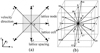 |
Fig. 1 Velocity sets of D2Q9 (a) and D3Q19 (b). |
2.2 Lattice Boltzmann method with the partially saturated cells method
2.2.1 Basic formulation
The LBM originated from lattice gas automata and its key concept involves developing simplified kinetic models that integrate the fundamental physics of microscopic or mesoscopic processes, thereby ensuring that the averaged macroscopic properties adhere to the intended macroscopic equations (Chen & Doolen 1998). The fundamental variable is the particle distribution function f (x, ξ, t), which represents the density in 3D physical and velocity space. Instead of the conventional Navier–Stokes equations, the Lattice Boltzmann equation (i.e., the Boltzmann equation with spatial and temporal discretization) is used in LBM (Chen & Doolen 1998):
 (6)
(6)
where the first equation represents the collision step and the second one represents the streaming step, respectively. The subscript i represents the ith direction. The vector ei is the direction of the discretized direction, and the coordinates of the nearest neighbor points around point x are x + ei. Qi is the collision operator, which represents the change rate of the distribution function. Δx and Δt are space and time increments, respectively. The notation DdQq represents the q-velocity model in d-dimensional space. Figure 1 shows the velocity sets of the D2Q9 and D3Q19 models, namely a nine-velocity model in 2D space and 19-velocity model in 3D space, respectively.
The density, ρ, and the velocity, u, are defined as particle velocity moments of the distribution function (Chen & Doolen 1998):
 (7)
(7)
In other words, the values of the macroscopic physical quantities are calculated based on the distribution function.
The expression of the collision operator Ωi mentioned above is complex and difficult to solve. Multiple simplified expressions have been derived based on different models to make the calculation simple enough. The Bhatnagar–Gross–Krook (BGK) collision operator (Bhatnagar et al. 1954) is a single relaxation time model that captures the relaxation of the distribution function toward the equilibrium distribution (Krüger et al. 2017). It can be expressed as
 (8)
(8)
where Δt is the time increment in LBM, and τ is the relaxation time, which determines the transport coefficients such as viscosity and heat diffusivity (Krüger et al. 2017). The equilibrium distribution,  , for an incompressible flow (i.e., the Mach number <<1) is given as (He & Luo 1997)
![Mathematical equation: $f_i^{{\rm{eq}}} = {\omega _i}\left\{ {\rho + {\rho _0}\left[ {{{({e_i} \cdot u)} \over {c_s^2}} + {{3{{({e_i} \cdot u)}^2}} \over {2c_s^4}} - {{{u^2}} \over {2c_s^2}}} \right]} \right\},$](/articles/aa/full_html/2024/11/aa49759-24/aa49759-24-eq15.png) (9)
(9)
where ρ and ρ0 are the local fluid density and the system’s average density, respectively. u is the local velocity and ωi is the weight coefficient in the ith direction. cs is the lattice sound speed, and varies from different discretizations of the continuum phase space. And the pressure is given by 
The BGK model is a simple and efficient way to simplify the collision operator. However, its accuracy and stability will reduce under large viscosities and small viscosities, respectively (Krüger et al. 2017). Hence, the multiple-relaxation-time (MRT) model is also applied as a supplementary method to overcome these problems.
The collision operator in the general MRT algorithm can be written as (d’Humières 2002)
 (10)
(10)
where M and M–1 is the transformation matrix and its inverse matrix, which transforms population space to moment space and back, respectively, based on the Gram–Schmidt procedure. The transformation matrix for multiple velocity sets can be found in d’Humières (2002), Suga et al. (2015) and Yang et al. (2012). R = diag (r1, r2,…, rq) is the relaxation matrix and r1, r2,…,rq are relaxation factors (see Suga et al. 2015 and d’Humières 2002 for more details).
2.2.2 Partially saturated cells method
The partially saturated cells method (PSM; Noble & Torczynski 1998) is also referred to as the immersed moving boundary method. Applying this method, the solid phase is resolved into each computation cell in the form of volume fraction ε. It is defined as the ratio of the volume of a fluid cell occupied by a specific particle to the whole cell volume. Figure 2 illustrates the interaction of a particle with a fluid cell. The fill level is used to modified the collision operator mentioned above and to evaluated the interaction forces between the two phases (Rettinger & Rüde 2017).
An essential procedure of PSM is calculating the volume fraction, ε, which needs to be recalculated at each time step once any particle moves. A cell-decomposition-based method (Owen et al. 2011) was applied in this study. In this method, a fluid cell is divided into equal-sized sub-cells, as shown in Fig. 3. An inside– outside algorithm is performed on each sub-cell center and the volume fraction, ε, is then calculated as as the ratio of the number of inside sub-cells to the total number of sub-cells. To obtain ε with a higher level of accuracy, a larger number of sub-cells is needed. However, this will take a longer computational time due to the increased effort needed to calculate and compare the distances between the center of the particle and the center of each sub-cell.
Therefore, we propose a novel algorithm for the rapid calculation of ε. As shown in Fig. 2, the volume fraction is influenced by the length ratio of the particle diameter to the side length of the fluid cell, and the position of the particle measured in the spherical coordinate system (cylindrical coordinate system for 2D conditions) with the center of the cell as the origin, including r, θ and ϕ. That is, the volume fraction is a function of the size ratio, the center–center distance and the two angles. We calculated the variance and the average value of each group of volume fraction results with the same size ratio and center–center distance and with two different azimuthal angles. The maximum standard deviation is 0.0192, which meets the requirement of the accuracy. Consequently, it can be concluded that the volume fraction exhibits minimal variation with respect to θ and φ. Thus, we can simplify the volume fraction as a function solely of the size ratio and the center–center distance. Subsequently, we constructed a dataset that correlates the volume fraction with the size ratio and center–center distance using the sub-cell method described above. During simulations, this predefined dataset was employed, and interpolation was used to calculate the corresponding volume fraction values.
To evaluate the efficiency of the approach, we conducted tests on one million randomly generated scenarios, using different size ratios, center–center distances, and angles. The interpolation method was compared with the supersampling method under four different conditions. The results of the test are listed in Table 1. t represents the CPU time it takes to conduct one million volume fraction calculations and E(Errɛ) means the expectation of the volume fraction error. The results indicate that the presented approach is able to significantly increase the efficiency of the volume fraction calculation, especially for 3D calculations. This improvement is essential for long-term and large-scale simulations. For example, a minimum of 216 (63) calculations are needed in each DEM time step when calculating the volume fractions of one particle under the condition that the lattice resolution is 5. If a simulation involves 10 000 particles and requires 10 000 integration iterations, the proposed method can save at least two hours. The time-saving potential of the interpolation method is even more pronounced with larger particle counts and extended simulation durations.
With the obtained volume fraction, the general expression of the modified collision operator is
 (11)
(11)
where s is the sth particle that occupies the local fluid cell. Bs is a weighting function related to the volume fraction ε and is given as
 (12)
(12)
and for a fluid cell, B = Σs Bs. The collision operator of the fluid phase  has been given in Sect. 2.2.1. The collision operator Ωi in Eq. (6) is replaced by
  in Eq. (11) when solid phase exists in the fluid calculation domain. The expression of the operator applied in this work is (Noble & Torczynski 1998)
![Mathematical equation: $\Omega _{i,s}^{{\rm{solid}}} = f_i^{{\rm{eq}}}\left( {\rho ,{{\bf{u}}_{\rm{s}}}} \right) - {f_q}\left( {{\bf{x}},t} \right) + \left( {1 - {{\Delta t} \over \tau }} \right)\left[ {{f_q}\left( {{\bf{x}},t} \right) - f_q^{{\rm{eq}}}\left( {\rho ,{{\bf{u}}_{\rm{f}}}} \right)} \right],$](/articles/aa/full_html/2024/11/aa49759-24/aa49759-24-eq22.png) (13)
(13)
where uf and us are local velocities of solid phase and fluid phase, respectively. The equation of the macroscopic velocity also needs to be modified when a solid phase exists in the fluid phase using the PSM:
 (14)
(14)
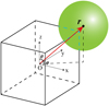 |
Fig. 2 DEM sphere interacting with a LBM cell (the cube). The dashed blue lines represent the portion of edges covered by the sphere. The center of the sphere is located at the spherical coordinate whose origin is at the center of the cell. |
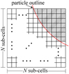 |
Fig. 3 Sub-cells in a fluid cell (the square). |
Comparison of the interpolation method and the supersampling method.
2.2.3 Boundary conditions
In LBM simulations, the application of boundary conditions entails the acquisition of the unknown populations at the lattice points residing along the boundary. When simulating the fluid–particle interactions on active comets, it is essential to consider various types of boundaries, including velocity boundaries, pressure boundaries, wall boundaries, and periodic boundaries.
The Zou–He boundary condition, as introduced by Zou & He (1997), is applied for open boundaries, including velocity boundaries and pressure boundaries. The speed u0 and the density ρ0 is fixed at the velocity boundary and the pressure boundary, respectively. Because the pressure is proportional to the density (given in Sect. 2.2.1), it is sufficient to give the density when applying the pressure boundary. Then Eq. (7) is solved with the given velocity and density. Additionally, the assumption that the bounce-back rule for the nonequilibrium part of the distribution function normal to the boundary is applied (i.e.,  ).
).
A straightforward periodic boundary condition is implemented into our code. The unknown populations  obtained after the collision step are determined by the corresponding populations at the opposite side of the domain. That is, if the length of the domain in a particular direction is L, the unknown populations can be expressed by
  .
.
The bounce-back formula is applied for Dirichlet boundary condition with a prescribed wall velocity, which is expressed as  (Krüger et al. 2017). The subscript w indicates the properties defined at the wall location.
2.2.4 Interaction force calculation
The hydrodynamic force acting upon a particle can be computed utilizing the previously derived quantities  and Bs. The last term in Eq. (11),
  , signifies the extent of disruption caused to the fluid as a result of the existence of solid particles. Therefore, the hydrodynamic force is the accumulation of momentum transfer across numerous lattice directions within the vicinity of n lattice cells occupied by the solid particle (Yang et al. 2019), which gives
 (15)
(15)
The hydrodynamic torque is the cross-product of the lever arm and the corresponding force, which can be written as
 (16)
(16)
where xs and xp are the center of the sth fluid cell occupied by a particle and the center of the particle, respectively. The subscript  represents the opposite direction of the vector.
We note that the calculation process outlined does not incorporate any empirical model representing fluid–solid interaction forces, such as a drag force model. Therefore, the obtained force in LBM is a product of “direct” simulation, devoid of reliance on hypothetical force models. This methodology extends beyond the calculation of forces acting solely on particles; indeed, it enables the direct computation of forces on solid structures with any shape. The steps needed are simply to calculate the volume fraction of each cell based on the shape.
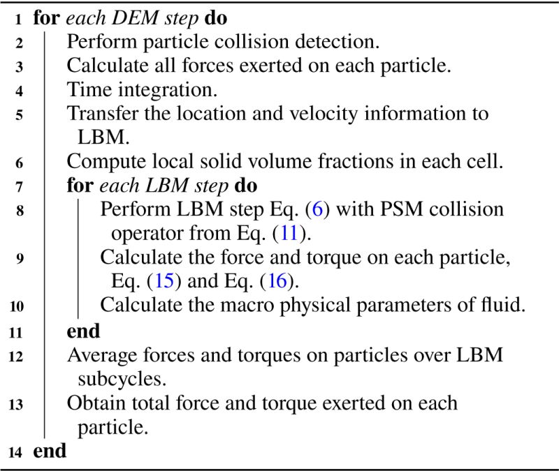
2.3 LBM-DEM algorithm summary
In the process of simulation implementation, a crucial parameter is the time step, which not only affects the accuracy of the simulation but also influences the computational resources consumed. A prevalent strategy for increasing the time step of DEM and thus saving resources involves the “softening” of particles, achieved through the reduction of the Young’s modulus pertaining to the material constituting the particles. However, in LBM simulations, dimensionless parameters are applied rather than physical units. The time coefficient ctime is determined based on the values of length coefficient clength and kinetic coefficient cv, and it is calculated as
 (17)
(17)
where ctime = treal/Δt, clength = lreal/Δx and cv = Vreal/vLBM, respectively. The time step of DEM is typically larger than that of LBM in our simulations. As a result, to achieve a stable flow field within each DEM time step, multiple iterations of LBM are required. Therefore, we can further enhance computational efficiency by judiciously reducing the number of LBM iterations per DEM time step.
The approach proposed in this paper is summarized in algorithm 1. The LBM with PSM is implemented into the selfdeveloped code LBMCoupler, integrated with the preexisting DEM code DEMBody1 (Cheng et al. 2021, 2022, 2023).
3 Model validation
Our code LBMCoupler employs both 2D and 3D models to accommodate a broader range of scenarios. In order to corroborate the efficacy of the coupling algorithm, we conducted three test simulations: the first involves an oscillating cylinder positioned at the center of a stationary fluid domain, the second features a stationary sphere subjected to a uniform flow environment and the third is the simulation of a particle transport process in a flume.
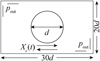 |
Fig. 4 Schematic of the oscillating cylinder immersed in the static flow. |
3.1 Flow induced by an oscillating cylinder
The first validation simulation involves a mobile body subjected to prescribed motion. The settings refers to that in Majumder et al. (2022): a cylinder with a diameter of d within a domain of size 30d × 20d. The cylinder is initially located at the center of the fluid domain as shown in Fig. 4 and subjected to a harmonic oscillation described by the following form,
 (18)
(18)
where Xc0 is the initial position of the cylinder, set to 15d. The recurring motion of the cylinder initiates the flow of fluid, and the fluctuating hydrodynamics can be described in terms of the Reynolds number (Re = U0d/v) and the Keulegan-Carpenter number (KC = U0/fd), where U0 is the peak velocity. Here the value of KC = 5 and Re = 100 are applied. The diameter of the cylinder d is 0.5 m, and the kinetic viscosity v is 1.0 × 10⁻⁶ m2/s, which is close to that of the water. The peak velocity U0 is 1.0 × 10⁻³ m/s and the frequency f is 2 × 10³ Hz. Pressure outlet boundary conditions are implemented at all the four domain boundaries.
Figure 5 displays velocity vectors and streamlines near the cylinder at three different phase angles of the cylinder’s oscillation. In the method we employed, the grid points inside the solid particles undergo collision and migration processes similar to those outside the particles. This approach is in contrast to the momentum exchange method, where fluid and solid points are entirely distinguished. Hence, within the region occupied by the cylinder in the figure, there are arrows representing fluid velocity. However, to enhance the visual distinction between the interior and exterior of the solid region while simultaneously illustrating the “fluid” velocity inside, this area has been treated with partial transparency. The close alignment between the experimental and numerical findings is affirmed by the comparisons presented in Fig. 5, which shows the results in Dütsch et al. (1998) and this work across three phase angles of the cylinder’s oscillatory motion. The streamline figures show that asymmetric vortices, which change over time, are generated on both sides of the moving cylinder at the three phase angles. It can be observed that the shape of the vortices and the streamlines exhibit fairly consistent match. This congruence suggests that our computational code is a credible tool for accurately simulating the flow field around moving objects.
Beyond the flow field computations, the calculation of the interaction forces between the fluid and particles needs to be validated as well. Here we focused on the force coefficients (Cd = 2F/pU2d for 2D) against time to calibrate the accuracy of our simulations. F is the force acting on a cylinder of unit length and U is the peak velocity the cylinder. Figure 6 shows that our results compare well with previous computational and experimental data, both in terms of the trend variation and the magnitude of the absolute values. We note that the results in Dütsch et al. (1998) are for periods after initial transient flows. Hence, we cut off the transients for the first several periods, represented by the period of t/T < 1.0, of our results in Fig. 6. The maximum absolute value of the drag coefficient is about 3.2, consistent with the value measured in previous experiments and simulations. We note that some discrepancies are indeed observed, particularly around the peaks and troughs of the Cd curve. This could potentially be attributed to factors such as the discetization of the movement of the cylinder and the selection of the time step.
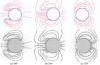 |
Fig. 5 Comparison of velocity vectors and streamlines in the vicinity of the cylinder for Re = 100 and KC = 5 between this work (the first row) and Dütsch et al. (1998, the second row) at (a) 180°, (b) 210°, and (c) 330°. The blue arrows are the velocity vectors, the red curves are the streamlines, and the black circle is the cylinder. |
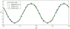 |
Fig. 6 Comparison of variation of streamwise drag coefficient, Cd, with respect to the time cycle between this work and Dütsch et al. (1998), Suzuki & Inamuro (2011), and Majumder et al. (2022). |
3.2 Uniform flow past a stationary sphere
The flow around a stationary sphere serves as a benchmark problem in the field of hydrodynamics. Figure 7 illustrates the 3D domain used in this validation simulations. The fluid domain is 20d in length, 5d in width, and 5d in height. At the inlet and outlet, velocity boundary conditions and pressure boundary conditions are respectively imposed. Four surrounding boundaries are subjected to periodic boundary conditions. A sphere, possessing a diameter denoted as d, is situated within the fluid domain. The distance from the center of the sphere to the inlet is 2.5d, with the sphere’s center aligning at the midpoint of the x-axis direction section.
The drag coefficients (Cd = 8F/ρU2πd2 in the context of 3D conditions) are computed across varying Reynolds number scenarios, derived from the simulation results. As mentioned algorithm 1, F is the time-averaged force calculated using Eq. (15) after the flow over the sphere reaches a steady state (i.e., when the drag force reaches stability over time). The Reynolds number is defined by the expression Re = Ud/ν, where d signifies the diameter of the sphere, and ν represents the kinematic viscosity of the fluid. Consequently, adjustments to the fluid velocity at the inlet are made to systematically vary the Reynolds number in the simulations. Figure 8a shows that the results obtained align well with the variation of drag coefficient with Reynolds number observed in previous works.
Moreover, we checked the influence of lattice resolution on the accuracy of the computational outcomes. Figures 8b and c illustrate two conditions of lattice resolution, 5 and 10, respectively. It is evident that higher resolution leads to improved accuracy, but within the resolution range we employed, the errors with respect to experimental measurements do not exceed 5%, which falls within an acceptable range. However, higher precision also entails larger computational expenses. Specifically, when the resolution is doubled, the requisite number of lattice points expands by a factor of eight in the context of 3D conditions, which means more than an eightfold increase in computational time. Therefore, a lattice resolution of 5 is predominantly employed in following simulations.
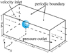 |
Fig. 7 Domain used in the validation simulation of the flow past a stationary sphere. |
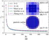 |
Fig. 8 Validation simulation results in the context of 3D conditions. (a) Comparison of the streamwise drag coefficient versus the Reynolds number in this work and in Schiller & Naumann (1935), Morsi & Alexander (1972), and Zhang & VanderHeyden (2002). (b and c) 2D representations depicting a DEM sphere mapped onto the LBM lattice grid at a lattice resolution of N = 5 and N = 10, respectively. |
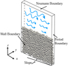 |
Fig. 9 Simulation domain of the validation simulations. |
3.3 Particle transport in a flume
In addition to running simulations of a single particle (or a cylinder), we validated our method by simulating sediment transport processes. Benavides et al. (2022) and Deal et al. (2023) undertook experimental investigations into bedload sediment transport using glass spheres within a confined flume. Zhang et al. (2022) simulated the transport process based on the experiment and calculated the transport flux versus the fluid shear stress. Here we conducted corresponding LBM-DEM simulations, with the settings based on those in Zhang et al. (2022). The validation result was evaluated by comparing the time-averaged sediment transport rates versus bed shear stress.
Figure 9 illustrates the simulation domain. Particles are located in the flume and fluid flows into the flume from the upstream. Particles are able to be moved when the fluid velocity is large enough (i.e., the transport flux increases when the fluid shear stress reaches a certain value). The particle motion is recorded by high-speed cameras in experiments (Deal et al. 2023) and it is more convenient to calculate the flux based on the particle motion by numerical simulations.
The particle phase consists of 903 spheres with an average diameter (dp) of 4.95 mm and a density (ρs) of 2550 kg/m3. Both the sphere-sphere and the sphere–wall friction coefficients are 0.5, and the restitution coefficient of the particles is 0.93. The simulated domain has a length of 118.8 mm and height of 148.5 mm. The width is slightly wider than two times of the average particle diameter and is 12.5 mm. Period boundary conditions are applied in the streamwise direction. The Neumann boundary condition is applied at the top of the domain, and the no-slip wall boundary conditions are applied in the bottom and two sides.
In the experiments, the flume is positioned at a specific angle relative to the ground. Hence, the gravity 𝑔 = 9.8 m/s2 is imposed at an angle of slope S with respect to the vertical axis of the simulated domain and the flow is driven by the gravity component parallel to the streamwise. The dimensionless sediment transport rate and the dimensionless bed shear stress are calculated, respectively, as
 (19)
(19)
and
 (20)
(20)
where qs and τb are the sediment volume flux per unit width and the bed shear stress, respectively. The fluid is water and the fluid density ρ is 1000 kg/m3. τb and qs are calculated as (Zhang et al. 2022)
 (21)
(21)
and
 (22)
(22)
where S is the slope of the flume. H is the height from the fluid surface to the bed surface. L and W are the simulated domain length and the fume width, respectively. Vi is the streamwise velocity of the ith particle.
Due to the limit of the calculation resource, we selected five different slopes for our simulations, corresponding to dimensionless shear stress τ* = 0.023, 0.028, 0.035, 0.047, and 0.068. The simulation duration is 30 s, with the last 10 s of data used to calculate the average values. The initial condition sets the particles distributed randomly with zero velocity and stationary fluid.
The outcomes achieved through our method, along with the simulation results of Zhang et al. (2022) and the experimental results of Deal et al. (2023), are presented in Fig. 10. When the dimensionless shear stress is low enough, particle movement is minimal, leading to a low dimensionless particle flux, consistent with the observations from Zhang et al. (2022). As the shear stress increases, particles begin to move and the flux increases rapidly. The results of our simulations show strong quantitative agreement with both the experimental results and the existing simulations. This consistency verifies the accuracy of our method and the reliability of out code.
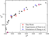 |
Fig. 10 Time-averaged dimensionless particle flux versus the dimensionless shear stress from this work (red circle), the experimental results of Deal et al. (2023, black cross), and the simulation results of Zhang et al. (2022, blue × mark). |
4 Application to comet 67P
When comet 67P is closer to the sun, its surface experiences periodic winds due to its rotation. Winds cause particles on the surface to start moving, leading to geomorphic changes such as the formation and migration of sand ripples (Jia et al. 2017). This phenomenon is a typical particle two-phase flow process. Our proposed approach can be used for the study of this problem. In this section we simulate the fluid flow over a simplified regolith layer as a preliminary application of the LBM-DEM framework, showcasing the efficacy of this method in modeling particle–fluid interactions on active small celestial bodies. And systematic simulations were conducted to estimate the threshold velocity for initiating particle movement on comet 67P.
4.1 Basic physical parameters
The gravitational force on comet 67P is exceedingly weak owing to its kilometer-scale dimensions, and its magnitude has been assessed through diverse methodologies (Sierks et al. 2015; Sachse et al. 2022). Here we used a value of 2 × 10⁻⁴ m/s2 in our simulations (Jia et al. 2017). The properties of the regolith grains were set to be similar to those on comet 67P (i.e., a Poisson ratio of 0.3 and a bulk density of 2400 kg/m3; Pätzold et al. 2016). According to Hertz’s theory, the time step in DEM simulations is determined by the Young’s modulus of the material and the maximum relative velocity among particles; that is, higher stiffness and collision velocities result in smaller time steps and longer computational costs. Therefore, in the framework of DEM simulations, a softened Young’s modulus, rather than its actual value, is typically employed to avoid long computation times. However, this softening must be moderated to ensure that the maximum overlaps between particles does not exceed the threshold of 5% of their radius, a critical constraint for maintaining the fidelity of the simulations. Given the relatively low collision velocities (below 0.1 m/s) in our simulation scenarios, a Young’s modulus of 106 Pa is implemented. Consequently, the DEM time step is set to 4 × 10⁻⁴ s.
In addition to the parameters mentioned above, the three key material properties of regolith grains mentioned in Sect. 2.1 (i.e., µ, β, and c) need to be determined. The calculated mean landslide apparent friction angle on comet 67P is 34° as reported by Lucchetti et al. (2019). Here we adopted both the sliding friction coefficient and the rolling friction coefficient of 1.0, which is equivalent to an internal friction angle of ~32° as calibrated in Cheng et al. (2023). Regarding the cohesion strength at the surface of comet 67P, there lacks a precise value for application. Attree et al. (2018) approximated the minimal tensile strength required on the surface to uphold overhangs and prevent them from collapsing under their gravitational forces. This study suggests that a minimal strength of around 1 Pa could be sufficient, with potential variations ranging from 1 to 5 Pa to sustain a one- meter-length overhang. Given that the Hapi region of comet 67P is characterized by its smooth, dust-covered terrain and absence of steep inclines (Attree et al. 2018), it is reasonable to assume that the cohesion strength of this area would not exceed 1 Pa. Therefore, for our simulations, the micro cohesion strength is set to be 39 Pa, corresponding to a macro cohesion strength of 0.98 Pa according to Eq. (5), which aligns with the estimated range for the surface of comet 67P.
Due to the limitations of computational resources, the simulations are constrained to a limited region on the surface of 67P, which is 60 cm in length, 30 cm in width and 11 cm in depth, as shown in Fig. 11. The average diameter of the particles is 2 cm and the regolith layer consists of 2023 spheres. Periodic boundary conditions are enforced in the x-direction, aligning with the mean flow direction, to eliminate the artificial effects of confining boundaries. Smooth wall boundary conditions are enforced in the two y-direction surfaces to eliminate the lateral forces and ensure that particles do not leave in the y-direction. A coarse wall is located at the bottom of the regolith layer. As illustrated in Fig. 11, particles that are closely attached to the bottom boundary (blue particles) are set to be immobilized. This setup can better depict the regolith layer on the surface of small celestial bodies under real conditions.
The wind traverses above the regolith layer, predominantly orienting along the direction of the x-axis. The fluid properties are chosen to mimic those observed on comet 67P at perihelion, particularly under the local afternoon conditions (Jia et al. 2017), with a density of 1 × 10⁻⁵ kg/m3. At the inlet, the velocity boundary condition is enforced, while the outlet is governed by the pressure boundary condition. As illustrated in Fig. 11, a velocity profile based on the principles of viscous fluid boundary layer theory is imposed at the inlet. Specifically, a linear velocity profile within the viscous sub-layer and a logarithmic profile extending far from the surface are applied, respectively.
The kinetic viscosity of the fluid can be calculated as (Jia 2016)
 (23)
(23)
where Vth is the thermal velocity and l is the mean free path. According to the estimation in Jia et al. (2017), the kinetic viscosity of the gas is about 1.67 m2/s. The character length is the average diameter of the particles and the velocity is about 30 m/s. Hence, the Reynolds number is about 0.36. The ratio of the particle density to the gas density is 2.4 × 10⁸ and the Galileo number is 0.1377.
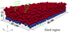 |
Fig. 11 Initial regolith layer. The blue particles are fixed during the calculation process, while red particles can move. A schematic diagram depicting the velocity profile and taking boundary layer effects into account is also drawn (green arrows). |
4.2 Data processing method
To determine the threshold quantitatively, a standard need to be established. Here the effective number of moving particles (neff) is applied based on the transported grains per unit area introduced in Durán et al. (2012), and is given as
 (24)
(24)
where up is the speed in the x-direction of a particle. The neff is measured from each simulation result. And the graph of the effective number versus shear velocity can be obtained. Hence, the threshold velocity can be determined according to the trend of the effective number.
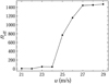 |
Fig. 12 Effective number of moving particles versus shear velocity. |
4.3 Estimation of the threshold velocity on comet 67P
The dynamical evolution of the regolith layer under rarefied traverse wind with various velocities is shown in supplementary online movies. Initially, the fluid field is at rest, that is to say, the velocity at each lattice point is zero in each simulation. Then, the velocity of the mean flow of the inlet boundary is set to undergo a gradual increase until it attains the predetermined maximum value. This maximum shear velocity is varied from 21 m/s to 29 m/s in intervals of 1 m/s, which enables the identification of the threshold wind velocity required to mobilize the particles.
Figure 12 shows the effective number of moving particles versus the shear velocity. When the flow velocity is sufficiently low (i.e., the shear velocity is between 21 m/s and 24 m/s), the effective number of the moving particles is relatively low. And as Fig. 13a shows, only a few particles have moved from their original positions when the shear velocity is 24 m/s. This variation can be attributed to the unique conditions experienced by individual particles within the regolith layer, rather than the dynamical state of the whole regolith layer. For example, some particles may be positioned above the average layer height or exhibit a relatively low equivalent strength compared to the average due to the fact that there is less contact area. Consequently, even under relatively low wind speeds, some isolated particles may begin to move. However, these isolated instances do not alter the overall static dynamical state of the particle layer; that is, the majority of particles remain in static.
With the increase in the wind velocity, a larger number of particles are set into motion within the same duration, leading to a rapid increase in the effective number of moving particles within the simulation duration. This transition indicates that particle movement has become a critical factor, marking a significant shift in the dynamical state of the regolith layer. Figure 13b shows the regolith layer at 30 s under the condition that the shear velocity is 25 m/s. Because of the high cohesion strength, the cohesion force dominates the resistance of the movement of the particles. However, the influence range of the cohesion force is small (one diameter of the particle). Hence, when the particles have been moved (i.e., the inter-particle force has been overcome), the resistance caused by the cohesion force reduces rapidly. Therefore, it can be observed from the image that when the wind speed increases to a certain value, the curve undergoes a very noticeable change, from 24 m/s to 25 m/s. This indicates that a large number of particles begin to move under the driving force of the gas, identifying this point as the threshold velocity. Hence, the threshold velocity is determined to be about 25 m/s according to Fig. 12. This approach ensures a more precise estimation of the threshold velocity for initiating particle motion under wind influence.
In addition to determine the threshold velocity, these simulations also reveal dynamical details of the particle layer erosion process under wind influence. Figure 14 shows the flow field and the streamlines under the condition of 24 m/s and 25 m/s at 30 s, respectively. The flow over the regolith layer exhibits laminar characteristics when the shape of the layer change little. The streamlines are relatively smooth, and the farther away from the layer, the higher the fluid velocity. As the wind velocity increases, some particles are detached from the surface of the particle layer due to the force exerted by the fluid. Since the velocity of the fluid is much higher than the velocity of the particles, the velocity of the fluid around the particles is lower than the velocity of the fluid away from the particles, which in turn appears as blue color in the lower one of Fig. 14. In addition, the presence of the flow past body around the particles can be seen through the streamlines, which is derived from the presence of particles.
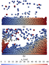 |
Fig. 13 Regolith layer under two different shear velocity conditions: (a) 24 m/s and (b) 25 m/s at 30 s. The color of the particles represents the original x-position (x0). |
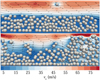 |
Fig. 14 Flow field at the simulation time of 30 s under the condition of a shear velocity of 24 m/s (the upper image) and 25 m/s (the lower image). |
4.4 Discussion
The computation of the temporal evolution of vapor velocity over the surface of comet 67P throughout a complete comet day is undertaken through calculations grounded in the thermal equilibrium model, porous layer model, and the turbulent boundary layer model, as expounded upon in detail in Jia et al. (2017). The results indicate a dynamic pattern of wind velocity near the comet’s surface: it starts at zero at sunrise, increases to a peak velocity of 75 m/s near perihelion, and then declines back to zero, remaining there throughout the night. This pattern suggests that for approximately 22% of the comet’s 12.4-hour day, the surface wind velocity exceeds our estimated threshold for sediment transport. This observation confirms that there is indeed a significant portion of the comet day during which sediment transport is viable, given the wind velocities surpass the identified threshold. The observation of the formation and active evolution of sand ripples on the surface of the comet is consistent with this inference. Therefore, the findings from this study provide a foundational assessment of the fluid environment on comet 67P. This validation underscores the utility of our methodology for exploring the dynamics of fluid–particle interactions in the context of active small celestial bodies.
Our method provide a useful simulation tool and there is no need to consider multiple types of interaction forces specially because no force model is needed in the presented method of force calculation as mentioned in Sect. 2.2.4. For example, the presence of a fluid velocity gradient along the normal direction of the regolith surface layer leads to lift forces on the particles. The significant velocity gradient adjacent to the surface, coupled with the fluid’s viscosity, makes the lift forces much large. We also observed in the simulation that some particles will move upward while traversing along the fluid flow direction. Separation of these rising particles from the regolith layer reduces their interactions, including cohesion and friction between particles. These complex dynamical effects are challenging to accurately incorporate within theoretical derivations. For instance, Jia et al. (2017) neglected the lift force exerted by the fluid on particles, and only a few spheres (Dey 1999) or circles (Shao & Lu 2000) were considered in theoretical derivations, which can lead to a biased result.
5 Conclusions
This paper advances a methodology for modeling fluid–particle interactions, particularly within the context of the environmental conditions prevailing on dynamic minor celestial bodies. This involves the synergistic integration of the LBM and DEM methods, which are implemented within our proprietary software framework LBMCoupler, which itself was derived from a preexisting SSDEM code, DEMBody. To substantiate the efficacy of this novel approach, we assessed the flow patterns induced by a 2D cylinder, determined the drag coefficient resulting from a uniform flow impinging upon a stationary 3D sphere, and quantitatively compared the transport rate of particles in a flume versus the fluid shear stress using experiments and existing simulations. Our findings show a strong concordance with the literature.
In a preliminary application, the simulation was conducted to elucidate the wind interaction on comet 67P using a regolith layer comprising 2023 particles. The evolutionary dynamics of the regolith layer exhibit discernible variations as the wind velocity increases. At lower wind velocities, particles proximate to the surface engage in a creeping motion, with occasional instances of particles achieving liftoff due to collisions with their counterparts. As the velocity increases, a large number of particles will be in motion, causing a change in the state of the particle layer, from which the threshold velocity can be determined. The calculated threshold velocity for wind-induced erosion means that sediment transport, which is the key mechanism in the formation of sand ripples, is able to take place on comet 67P. This validates the effectiveness of our approach and underscores the potential of our methodology for assessing threshold velocities for erosion and sediment transport. A more in-depth study of the threshold velocity of active small solar bodies will be presented in subsequent works.
The proposed methodology has significant potential for simulating fluid–particle interaction phenomena on active small celestial bodies. Future research should delve deeply into regolith transport, with a focus on investigating the morphological changes occurring on these active small bodies. However, the current scale of the regolith layer simulation is insufficient for a comprehensive analysis. To address this limitation, substantial improvements to the algorithm’s efficiency are essential. Additionally, the utilization of an unresolved methodology – wherein particles remain unresolvable to the fluid cell – coupled with the application of fluid-interaction models becomes crucial. This strategy is particularly relevant for accommodating scenarios with a higher number of particles and longer simulation times, and would enable the exploration of fluid–particle interactions on a much larger scale.
Data availability
The simulations were performed using the DEMBody and LBMCoupler codes in their custom version that includes the SSDEM and the LBM (see Sect. 2). The compiled version can be downloaded via https://github.com/gicyerlivan147/LBM-DEM-COMPILED
Movies linked to Sect. 4.3 are available at https://www.aanda.org
Acknowledgements
This work is supported by the National Natural Science Foundation of China under Grant 62227901. B.C. is also supported by the National Natural Science Foundation of China (No. 12202227) and the Postdoctoral Innovative Talent Support Program of China (No. BX20220164).
References
- Ai, J., Chen, J.-F., Rotter, J. M., & Ooi, J. Y. 2011, Powder Technol., 206, 269 [CrossRef] [Google Scholar]
- Attree, N., Groussin, O., Jorda, L., et al. 2018, A&A, 611, A33 [NASA ADS] [CrossRef] [EDP Sciences] [Google Scholar]
- Benavides, S. J., Deal, E., Rushlow, M., et al. 2022, Geophys. Res. Lett., 49, e2021GL096088 [NASA ADS] [CrossRef] [Google Scholar]
- Betat, A., Frette, V., & Rehberg, I. 1999, Phys. Rev. Lett., 83, 88 [NASA ADS] [CrossRef] [Google Scholar]
- Bhatnagar, P. L., Gross, E. P., & Krook, M. 1954, Phys. Rev., 94, 511 [Google Scholar]
- Bird, G. A. 1994, Molecular Gas Dynamics And The Direct Simulation Of Gas Flows (Oxford University Press) [Google Scholar]
- Chen, S., & Doolen, G. D. 1998, Annu. Rev. Fluid Mech., 30, 329 [CrossRef] [Google Scholar]
- Cheng, B., Yu, Y., Asphaug, E., et al. 2021, Nat. Astron., 5, 134 [Google Scholar]
- Cheng, B., Asphaug, E., Ballouz, R.-L., Yu, Y., & Baoyin, H. 2022, Planet. Sci. J., 3, 249 [NASA ADS] [CrossRef] [Google Scholar]
- Cheng, B., Asphaug, E., Yu, Y., & Baoyin, H. 2023, Astrodynamics, 7, 15 [NASA ADS] [CrossRef] [Google Scholar]
- Clark, A. H., Kondic, L., & Behringer, R. P. 2016, Phys. Rev. E, 93, 050901 [NASA ADS] [CrossRef] [Google Scholar]
- Claudin, P., & Andreotti, B. 2006, Earth Planet. Sci. Lett., 252, 30 [CrossRef] [Google Scholar]
- Deal, E., Venditti, J. G., Benavides, S. J., et al. 2023, Nature, 613, 298 [NASA ADS] [CrossRef] [Google Scholar]
- Dey, S. 1999, Appl. Math. Model., 23, 399 [CrossRef] [Google Scholar]
- d’Humières, D. 2002, Philos. Trans. Roy. Soc. Lond. A Math. Phys. Eng. Sci., 360, 437 [CrossRef] [Google Scholar]
- Durán, O., Andreotti, B., & Claudin, P. 2012, Phys. Fluids, 24, 103306 [CrossRef] [Google Scholar]
- Durán, O., Claudin, P., & Andreotti, B. 2014, PNAS, 111, 15665 [CrossRef] [Google Scholar]
- Dütsch, H., Durst, F., Becker, S., & Lienhart, H. 1998, J. Fluid Mech., 360, 249 [CrossRef] [Google Scholar]
- Fan, F., Parteli, E. J. R., & Pöschel, T. 2017, Phys. Rev. Lett., 118, 218001 [NASA ADS] [CrossRef] [Google Scholar]
- Greeley, R., & Iversen, J. D. 1985, Wind as a Geological Process: On Earth, Mars, Venus, and Titan, Cambridge Planetary Science Series (Cambridge [Cambridgeshire]; New York: Cambridge University Press) [CrossRef] [Google Scholar]
- Greeley, R., Iversen, J., Leach, R., et al. 1984, Icarus, 57, 112 [NASA ADS] [CrossRef] [Google Scholar]
- Guckenheimer, J., & Holmes, P. 1997, Nonlinear Oscillations, Dynamical Systems, and Bifurcations of Vector Fields, corr. 5th print edn., Applied Mathematical Sciences, No. v.42 (New York: Springer) [Google Scholar]
- He, X., & Luo, L.-S. 1997, J. Statist. Phys., 88, 927 [NASA ADS] [CrossRef] [Google Scholar]
- Hirabayashi, M., Scheeres, D. J., Sánchez, D. P., & Gabriel, T. 2014, ApJ, 789, L12 [NASA ADS] [CrossRef] [Google Scholar]
- Homayoon, A., Isfahani, A. M., Shirani, E., & Ashrafizadeh, M. 2011, Int. Commun. Heat Mass Transfer, 38, 827 [CrossRef] [Google Scholar]
- Jia, P. 2016, PhD thesis, Université Sorbonne Paris, France [Google Scholar]
- Jia, P., Andreotti, B., & Claudin, P. 2017, PNAS, 114, 2509 [NASA ADS] [CrossRef] [Google Scholar]
- Jiang, M., Shen, Z., & Wang, J. 2015, Comput. Geotech., 65, 147 [NASA ADS] [CrossRef] [Google Scholar]
- Kandhai, B., Derksen, J., & Van Den Akker, H. 2002, in Parallel Computational Fluid Dynamics 2001 (Elsevier), 199 [CrossRef] [Google Scholar]
- Kok, J. F., Parteli, E. J. R., Michaels, T. I., & Karam, D. B. 2012, Rep. Progr. Phys., 75, 106901 [CrossRef] [Google Scholar]
- Krüger, T., Kusumaatmaja, H., Kuzmin, A., et al. 2017, The Lattice Boltzmann Method: Principles and Practice, Graduate Texts in Physics (Cham: Springer International Publishing) [CrossRef] [Google Scholar]
- Lucchetti, A., Penasa, L., Pajola, M., et al. 2019, Geophys. Res. Lett., 46, 14336 [NASA ADS] [CrossRef] [Google Scholar]
- Majumder, S., Arnab, G., Dipankar, N. B., & Ganesh, N. 2022, Comput. Math. Applic., 110, 19 [CrossRef] [Google Scholar]
- Morsi, S. A., & Alexander, A. J. 1972, J. Fluid Mech., 55, 193 [CrossRef] [Google Scholar]
- Nie, X., Doolen, G. D., & Chen, S. 2002, J. Statist. Phys., 107, 279 [NASA ADS] [CrossRef] [Google Scholar]
- Noble, D. R., & Torczynski, J. R. 1998, Int. J. Mod. Phys. C, 09, 1189 [NASA ADS] [CrossRef] [Google Scholar]
- Owen, D. R. J., Leonardi, C. R., & Feng, Y. T. 2011, Int. J. Numer. Methods Eng., 87, 66 [NASA ADS] [CrossRef] [Google Scholar]
- Pätzold, M., Andert, T., Hahn, M., et al. 2016, Nature, 530, 63 [CrossRef] [Google Scholar]
- Rettinger, C., & Rüde, U. 2017, Comput. Fluids, 154, 74 [CrossRef] [Google Scholar]
- Rozitis, B., MacLennan, E., & Emery, J. P. 2014, Nature, 512, 174 [CrossRef] [Google Scholar]
- Sachse, M., Kappel, D., Tirsch, D., & Otto, K. A. 2022, A&A, 662, A2 [NASA ADS] [CrossRef] [EDP Sciences] [Google Scholar]
- Sánchez, P., & Scheeres, D. J. 2014, Meteor. Planet. Sci., 49, 788 [Google Scholar]
- Schiller, L., & Naumann, A. 1935, Z. Vereins Deutsch. Ing., 77, 318 [Google Scholar]
- Shao, Y., & Lu, H. 2000, J. Geophys. Res. Atmos., 105, 22437 [CrossRef] [Google Scholar]
- Sierks, H., Barbieri, C., Lamy, P. L., et al. 2015, Science, 347, aaa1044 [Google Scholar]
- Silvestro, S., Fenton, L. K., Vaz, D. A., Bridges, N. T., & Ori, G. G. 2010, Geophys. Res. Lett., 37, 2010GL044743 [CrossRef] [Google Scholar]
- Somfai, E., Roux, J.-N., Snoeijer, J. H., van Hecke, M., & van Saarloos, W. 2005, Phys. Rev. E, 72, 021301 [NASA ADS] [CrossRef] [Google Scholar]
- Stegner, A., & Wesfreid, J. E. 1999, Phys. Rev. E, 60, R3487 [NASA ADS] [CrossRef] [Google Scholar]
- Suga, K., Kuwata, Y., Takashima, K., & Chikasue, R. 2015, Comput. Math. Applic., 69, 518 [CrossRef] [Google Scholar]
- Sullivan, R., Banfield, D., Bell, J. F., et al. 2005, Nature, 436, 58 [NASA ADS] [CrossRef] [Google Scholar]
- Sundaresan, S., Ozel, A., & Kolehmainen, J. 2018, Annu. Rev. Chem. Biomol. Eng., 9, 61 [CrossRef] [Google Scholar]
- Suzuki, K., & Inamuro, T. 2011, Comput. Fluids, 49, 173 [CrossRef] [Google Scholar]
- Telfer, M. W., Parteli, E. J. R., Radebaugh, J., et al. 2018, Science, 360, 992 [NASA ADS] [CrossRef] [Google Scholar]
- Thomas, N., Davidsson, B., El-Maarry, M. R., et al. 2015, A&A, 583, A17 [NASA ADS] [CrossRef] [EDP Sciences] [Google Scholar]
- Udo, K., Kuriyama, Y., & Jackson, D. W. T. 2008, J. Geophys. Res., 113, F04008 [Google Scholar]
- Weitz, C. M., Plaut, J. J., Greeley, R., & Saunders, R. S. 1994, Icarus, 112, 282 [NASA ADS] [CrossRef] [Google Scholar]
- Yang, F., Shi, X., Guo, X., & Sai, Q. 2012, Energy Procedia, 16, 639 [NASA ADS] [CrossRef] [Google Scholar]
- Yang, G., Jing, L., Kwok, C., & Sobral, Y. 2019, Comput. Geotech., 114, 103100 [NASA ADS] [CrossRef] [Google Scholar]
- Zhang, Y., & Michel, P. 2021, Astrodynamics, 5, 293 [NASA ADS] [CrossRef] [Google Scholar]
- Zhang, D. Z., & VanderHeyden, W. 2002, Int. J. Multiphase Flow, 28, 805 [NASA ADS] [CrossRef] [Google Scholar]
- Zhang, Y., Richardson, D. C., Barnouin, O. S., et al. 2018, ApJ, 857, 15 [Google Scholar]
- Zhang, Y., Michel, P., Richardson, D. C., et al. 2021, Icarus, 362, 114433 [CrossRef] [Google Scholar]
- Zhang, Q., Deal, E., Perron, J. T., et al. 2022, J. Geophys. Res., 127, e2021JF006504 [NASA ADS] [CrossRef] [Google Scholar]
- Zou, Q., & He, X. 1997, Phys. Fluids, 9, 1591 [CrossRef] [Google Scholar]
Our code can be downloaded from the following website: https://bin-cheng-thu.github.io/dembody-code/
All Tables
All Figures
|
Fig. 1 Velocity sets of D2Q9 (a) and D3Q19 (b). |
| In the text | |
|
Fig. 2 DEM sphere interacting with a LBM cell (the cube). The dashed blue lines represent the portion of edges covered by the sphere. The center of the sphere is located at the spherical coordinate whose origin is at the center of the cell. |
| In the text | |
|
Fig. 3 Sub-cells in a fluid cell (the square). |
| In the text | |
|
Fig. 4 Schematic of the oscillating cylinder immersed in the static flow. |
| In the text | |
|
Fig. 5 Comparison of velocity vectors and streamlines in the vicinity of the cylinder for Re = 100 and KC = 5 between this work (the first row) and Dütsch et al. (1998, the second row) at (a) 180°, (b) 210°, and (c) 330°. The blue arrows are the velocity vectors, the red curves are the streamlines, and the black circle is the cylinder. |
| In the text | |
|
Fig. 6 Comparison of variation of streamwise drag coefficient, Cd, with respect to the time cycle between this work and Dütsch et al. (1998), Suzuki & Inamuro (2011), and Majumder et al. (2022). |
| In the text | |
|
Fig. 7 Domain used in the validation simulation of the flow past a stationary sphere. |
| In the text | |
|
Fig. 8 Validation simulation results in the context of 3D conditions. (a) Comparison of the streamwise drag coefficient versus the Reynolds number in this work and in Schiller & Naumann (1935), Morsi & Alexander (1972), and Zhang & VanderHeyden (2002). (b and c) 2D representations depicting a DEM sphere mapped onto the LBM lattice grid at a lattice resolution of N = 5 and N = 10, respectively. |
| In the text | |
|
Fig. 9 Simulation domain of the validation simulations. |
| In the text | |
|
Fig. 10 Time-averaged dimensionless particle flux versus the dimensionless shear stress from this work (red circle), the experimental results of Deal et al. (2023, black cross), and the simulation results of Zhang et al. (2022, blue × mark). |
| In the text | |
|
Fig. 11 Initial regolith layer. The blue particles are fixed during the calculation process, while red particles can move. A schematic diagram depicting the velocity profile and taking boundary layer effects into account is also drawn (green arrows). |
| In the text | |
|
Fig. 12 Effective number of moving particles versus shear velocity. |
| In the text | |
|
Fig. 13 Regolith layer under two different shear velocity conditions: (a) 24 m/s and (b) 25 m/s at 30 s. The color of the particles represents the original x-position (x0). |
| In the text | |
|
Fig. 14 Flow field at the simulation time of 30 s under the condition of a shear velocity of 24 m/s (the upper image) and 25 m/s (the lower image). |
| In the text | |
Current usage metrics show cumulative count of Article Views (full-text article views including HTML views, PDF and ePub downloads, according to the available data) and Abstracts Views on Vision4Press platform.
Data correspond to usage on the plateform after 2015. The current usage metrics is available 48-96 hours after online publication and is updated daily on week days.
Initial download of the metrics may take a while.