| Issue |
A&A
Volume 691, November 2024
|
|
|---|---|---|
| Article Number | A313 | |
| Number of page(s) | 7 | |
| Section | Astrophysical processes | |
| DOI | https://doi.org/10.1051/0004-6361/202348635 | |
| Published online | 21 November 2024 | |
Constraints on the accretion properties of quasi-periodic erupters from GRMHD simulations
1
Max Planck Institute for Astronomy, Königstuhl 17, 69117 Heidelberg, Germany
2
The Raymond and Beverly Sackler School of Physics and Astronomy, Tel Aviv University, Tel Aviv 69978, Israel
⋆ Corresponding author; This email address is being protected from spambots. You need JavaScript enabled to view it.
Received:
16
November
2023
Accepted:
14
October
2024
Abstract
Context. Some apparently quiescent supermassive black holes (BHs) at centers of galaxies show quasi-periodic eruptions (QPEs) in the X-ray band, the nature of which is still unknown. A possible origin for the eruptions is an accretion disk. However, the properties of such disks are restricted by the timescales of recurrence and the duration of the flares.
Aims. In this work, we test the possibility that the temporal properties of known QPEs can be explained by accretion from a compact accretion disk with an outer radius rout ∼ 40rg, and we focus on a particular object, GSN 069.
Methods. We ran several 3D general relativistic magnetohydrodynamic (GRMHD) simulations with the H-AMR code of thin and thick disks and studied how the initial disk parameters such as thickness, magnetic field configuration, magnetization, and Kerr parameter affect the observational properties of QPEs.
Results. We show that accretion onto a slowly rotating BH through a small, moderately thin accretion disk with an initially low plasma β can explain the observed time between outbursts and the lack of evidence for a variable jet emission. In order to form such a disk, the accreting matter should have a low net angular momentum. A potential source for such low angular momentum matter with a quasi-periodic feeding mechanism might be a tight binary of wind-launching stars. Apart from their primary application, our results can also be useful for general studies of systems with small accretion disks, in which evolution occurs very rapidly so that the disks cannot be considered stationary. For such systems, it is important to understand how the initial conditions affect the results.
Key words: accretion / accretion disks / black hole physics / magnetic fields / magnetohydrodynamics (MHD) / methods: numerical
© The Authors 2024
 Open Access article, published by EDP Sciences, under the terms of the Creative Commons Attribution License (https://creativecommons.org/licenses/by/4.0), which permits unrestricted use, distribution, and reproduction in any medium, provided the original work is properly cited.
This article is published in open access under the Subscribe to Open model.
Open access funding provided by Max Planck Society.
1. Introduction
Quasi-periodic eruptions (QPEs) were detected for the first time in the galactic nucleus of GSN 069 in 2019 (Miniutti et al. 2019). During the active periods, the observed X-ray luminosity increased by up to two orders of magnitude above its quiescent level, reaching a peak luminosity of Lx = 1042 − 1043 erg s−1. The source has also been detected at 6 GHz by the Very Large Array (VLA), and it has a persistent radio luminosity of Lradio ∼ 1.9 ⋅ 1036 erg s−1 and a corresponding jet power Pj ≈ 1041 erg s−1 (Miniutti et al. 2019). Later, four other sources with QPEs were found: RX J1301.9+2747, eRO-QPE1, eRO-QPE2, and XMMSL1 J024916.6−041244 (Giustini et al. 2020; Arcodia et al. 2021; Chakraborty et al. 2021). All four of these sources have similar variability patterns, namely, short X-ray outbursts (0.4–8 hours) separated by long quiescent states (2–19 hours). The durations of the outbursts, their amplitudes, and the recurrence times are not constant for a given source, and they change from burst to burst in such a way that the strongest QPE is followed by a longer recurrence time (Miniutti et al. 2019). The spectra in both the active and quiescent states are soft and well fitted by a blackbody with a temperature of kT ∼ 30 − 50 eV in the quiescent and kT ∼ 100 − 300 eV during the active states, although quiescent emission has not been detected from all sources. Assuming that the quiescent blackbody emission comes from inner accretion disk regions, one may estimate the black hole (BH) masses in the observed QPEs to be in the range MBH = 105 − few × 106 M⊙. All sources are associated with galactic nuclei, but their inferred masses are smaller than typical BH masses in AGNs. Another feature distinguishing these sources from classical AGNs is the lack of broad optical or UV emission lines, although in GSN 069 there are narrow-line regions that might indicate recent activity. According to Miniutti et al. (2019), the lack of variability in the radio source detected in GSN 069 implies that the production mechanism of the associated jet is likely unrelated to the QPE process. As we argue in this work, this may not necessarily be the case. The observed parameters of each of the five sources mentioned are given in Table 1.
Main observational parameters of the QPE systems.
Quasi-periodic eruptions are widely discussed in the community (e.g. Pan et al. 2022; Lu & Quataert 2023; Suková et al. 2021; Metzger et al. 2022; Ingram et al. 2021; Wang et al. 2022). A major challenge for any model involving disk accretion is the viscous timescale, which is determined by disk size and can easily exceed the observed duration of the outbursts. One possible scenario to explain it is that the outbursts originate from the innermost parts of the disk and are thus disconnected from the overall viscous time. For example, Pan et al. (2022) assumed that the QPEs are produced by radiation- or magnetic pressure-driven instabilities at the inner part of the accretion disk (see also Śniegowska et al. 2023). Lu & Quataert (2023) explained the QPEs with circularization shocks that take place during unstable mass-transfer events onto the BH from a star undergoing a Roche-lobe overflow (RLOF).
We discuss in more detail two works that are particularly relevant to our work. In the first, Metzger et al. (2022) considered two stars orbiting a BH on co-planar orbits, where at least the outer star is undergoing a RLOF. When the inner star passes between the outer star and the BH, the combined gravitational pull reduces the Roche-lobe radius of the outer star, causing a short-term increase in the mass transfer rate from the outer star. As a result, the accretion disk is loaded with fresh stellar material. In this model, the disk accretion is the source of the QPE, while the recurrence time is determined by the time interval between flybys of the two stars. In such a system, the accretion disk formed during the flybys could be considerably more compact due to the sideways gravitational pull of the second star, thus resolving the long viscous time problem.
In the second work, Krolik & Linial (2022) connected the origin of QPEs with the formation of a self-interacting shock in the accretion stream from a star orbiting the BH. In this model, it was assumed that a significant amount of the angular momentum of the matter is carried away by magnetic stresses so the shocked matter falls down onto the BH within the free-fall time. The existence of magnetic stresses suggests a prompt formation of an accretion disk, where the stresses are responsible for effective viscosity and thus for angular momentum distribution. From simulations of disk accretion, magnetic pressure is known to be limited by approximate equipartition, and the magnetization of the accretion flow itself is never very high. For the Krolik & Linial (2022) model to be successful, it is necessary for the accretion disk to accrete most of its mass during the recurrence time, again implying a small disk size.
Both of these works explain some observational features of the QPEs, such as the burst and recurrence times and the burst amplitudes. However, an important question remains regarding what happens to the matter during its accretion onto the BH. To account for the flare energy, an excess mass of ΔM ∼ 10−7 M⊙ must be transferred from the star to the disk in each cycle, corresponding to a mean mass transfer rate of ΔM/Trec ∼ 10−4 (ΔM/10−7 M⊙)(Trec/10 h)−1 M⊙/yr, where Trec is the flare recurrence time. If the accretion time is longer than the flare recurrence time, the mass of the disk will continuously increase until a quasi-steady state is established, where (on average) the rate at which mass is transferred to the disk is balanced by the rate of accretion onto the BH. This leads to a quiescent bolometric luminosity of Lb ≈ 1042 erg s−1, which may be consistent with the observed luminosity during minimum states in GSN 069 and RXJ 1301.9+2747, assuming a correction factor of a few between the UV and soft X-ray luminosities but not with the quiescent luminosity of other QPEs. Regardless of these observational constraints, in both models, the authors argued that it is necessary for the BH to accrete all the material within the timescale of the QPE cycle or even within the timescale of the flare itself. Metzger et al. (2022) made 1D semi-analytical calculations and showed that a significant part of the disk material will accrete onto the BH at timescales of less than a day (see Fig. 3 of their paper). Krolik & Linial (2022) did not attempt to model the infalling material beyond the point of self-intersection. A more self-consistent answer to this question can be found using numerical 3D simulations of the accretion flow.
In this work, we investigate whether the recurrence times can be explained by a disk accretion onto a BH without invoking additional physical entities. This general result has particular applications to the works of Metzger et al. (2022) and Krolik & Linial (2022). In a system with an orbital period Porb ∼ Trec ∼ 10 hours, the accretion disk size would typically be on the order of a hundred gravitational radii rg. Information about any changes at the outer boundary of the disk are transferred into the inner parts on viscous times associated with the outer disk radius, rout, which is too large to account for the QPE. An obvious way to account for this inconsistency is to assume that the disk is initially much more compact. In this paper, we consider accretion from smaller disks with outer radii rout ∼ 40rg and thicknesses h/r ∼ 0.1 − 1. The viscous times at the outer boundaries of these disks is 50/α0.1 hours, where α0.1 = α/0.1 is the viscosity parameter, comparable with the recurrence time. This disk size is consistent with the observed luminosities and blackbody temperatures, both in the quiescent and in the active states, meaning that the emitting region should be very compact and comparable to the innermost stable circular orbit size. In addition to the fact that such a disk has much shorter viscous timescales, the small size can also explain the lack of broad optical and UV emission lines that are produced in the outer parts of huge AGN disks. We did not study how such a small disk can be formed. Instead, we focus on the overall dynamics and timescale evolution of the accretion process. However, we mention a few possible formation paths for such a disk in the discussion. A more elaborated study of the flares associated with the disk should involve radiative processes, and this will be performed in the future papers.
In the next section, we describe the numerical models we used. In Section 3, we discuss how the disk parameters influence the accretion dynamics of the disk and its relation to the observational properties of the QPEs. We also use our simulations to explore the predicted jet power in order to explain the absence of variable jets in these systems. Finally, in Section 4 we summarize the results.
2. Models
We conducted multiple 3D general relativistic magnetohydrodynamic (GRMHD) simulations utilizing the H-AMR code (Liska et al. 2022), which is based on the original HARM code by Gammie et al. (2003) and Noble et al. (2006). All the main equations are given in those papers. The simulations were performed in spherical Boyer-Lindquist coordinates r, θ, ϕ. We invoked a standard Fishbone and Moncrief torus (Fishbone & Moncrief 1976) surrounding a Kerr BH with outflow, transmissive, and periodic boundary conditions in the r, θ, ϕ directions, respectively.
We used the units G = c = 1 and normalized all of our quantities by the BH mass MBH, 0 and maximal disk density ρ0. The adiabatic index in our simulations is γ = 4/3. The grid is evenly spaced in the angular directions, while the radial direction we use the following spacing for r < 400rg, we used a logarithmically spaced grid with a constant dr/r, and for r > 400rg the grid scales as dr/r = 4(log r)3/4. We set the basic resolution to Nr × Nθ × Nϕ = 192 × 132 × 128, where we applied an additional level of adaptive mesh refinement (AMR) in regions with ρ > 0.5ρ0, resulting in an effective resolution in the disk of Nr × Nθ × Nϕ = 384 × 264 × 512. The initial torus has an inner radius of rin = 8rg, and the gas pressure has a maximum at rmax = 14rg, so the outer boundary of the disk is about 40rg (see the description of all models in Table 2). The cell aspect ratio on the equatorial plane at r = rin is δr : rδθ : rδϕ = 1 : 0.69 : 0.71. Since the initial torus is not too large, we set the outer radial boundary at Rsim = 1000 rg. We ran one additional simulation of a thick disk with a larger outer boundary Rsim = 105rg to check for consistency and verified that the results remained unchanged. In most models (K1–K5), there is no radiation, so the disks are advection dominated Narayan & Yi (1995). In two models, K6 and K7, we cool down the gas to produce moderately thin disks with h/r = 0.3 and h/r = 0.1, respectively (Liska et al. 2021).
Details of the 3D simulations used in this paper and the main result.
The initial magnetic field in the torus contains only a poloidal component defined by the ϕ− component of the vector potential Aϕ. We considered two different initial magnetic field configurations (Fig. 1). The first configuration is a single loop defined by the vector potential:
 (1)
(1)
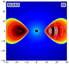 |
Fig. 1. Initial density distribution and magnetic field configuration in the thick disk models (K1–K5). Magnetic field lines are marked by solid black lines for clockwise oriented field, and dashed white lines are used for those in the counter-clockwise oriented field. In the thin disk simulations K6, K7, we used the same single loop initial conditions. The initially thick torus evolved into a thin disk because of the cooling within the first 500 dynamical times. |
Here, ρcut = 0.05ρ0 is the threshold density below which the magnetic field vanishes. The second configuration has multiple dipolar loops set by
 (2)
(2)
where Nloops is the number of the loops and
 (3)
(3)
with  ,
,  respectively denoting the inner and outer radii of the torus (or more precisely its magnetized section, defined by ρ > ρcut). In our simulations, we considered Nloops = 6 for model K2. The normalization parameter A0 was chosen to ensure the required initial ratio of gas to magnetic pressure is β = pg/pm ≥ βmin, where βmin is set by hand for every simulation (see Table 2). This form of magnetic potential gives an approximately constant β distribution in the disks, which is important for our ability to resolve the magneto-rotational instability (MRI; Balbus & Hawley 1991).
To compare our results with observations, we converted the code time units into physical ones using a characteristic BH mass, MBH, 0 = 106 M⊙, with an associated dynamical time, td = 4.93MBH/MBH, 0 s. We did not convert the mass accretion rate from the code units to the physical units because they depend on the disk density ρ0, which is a free parameter in our models. We emphasize that the accretion time depends on the disk geometry but not on ρ0. Therefore, Ṁ can be re-scaled by changing ρ0 without affecting the recurrence time. In reality, ρ0 can be inferred from the mean accretion rate (averaged over the orbital period of the donor star), which is determined by the rate of mass transfer from the star to the disk and should be ⟨Ṁ⟩ ∼ 10−4 M⊙ yr−1. We note that this quantity merely reflects the bolometric luminosity during quiescent states (i.e., between flaring states), thus setting a lower limit on the actual accretion rate during a flare.
3. Results
In this work, we focus on two observed properties of the QPE in GSN 069 and test what type of disks can reproduce them: (1) A recurrence time of Trec ∼ 10 hours, which is related to the disk accretion time. (2) The absence of a variable jet, which is connected with the electromagnetic (EM) energy output from the BH. To test each property, we divided our models into three groups:
-
We used models K2 and K3 to understand the effect of the magnetic field configuration.
-
We used models K1, K3, K4, and K5 to test the importance of the plasma β and the Kerr parameter a.
-
We used models K3, K6, and K7 to understand how the disk thickness, h/r, affects the accretion time and jet production.
For each model, we plotted the evolution of the mass accretion rate through the horizon in code units:
 (4)
(4)
where ρ is the proper mass density, ur is the r-component of the contravariant four-velocity,  is a solid angle differential area, and g is the metric determinant. The integral is taken on the BH horizon, defined by a sphere with a radius
  .
.
In order to check for the presence of a jet, we analyzed the accretion jet efficiency, ηa, which measures the electromagnetic power output from the BH horizon relative to the rest-mass energy flux that crosses the horizon. It is defined as
 (5)
(5)
where  is the rest-mass energy flow through the horizon and FEM = ∬[TEM]trdAΩ is the total EM power coming out of the BH horizon, with [TEM]tr = b2urut − brbt denoting the electromagnetic part of the rt component of the stress-energy tensor. Here, bi and bi are contravariant and covariant fluid-frame magnetic four-field components, and b2 = bibi Komissarov (1999), Tchekhovskoy et al. (2011).
The initial phase of magnetic field amplification in the disk sets the onset time of accretion onto the BH. As this time affects the overall lifetime of our transient disks, it is important to make sure that the magnetic field amplification is physical (i.e., driven by MRI in the disk). A standard way of evaluating this is to measure the quality factor, Qi, which measures the number of cells resolving the initial MRI wavelength in the i = r, θ, ϕ direction:
 (6)
(6)
Here, vA, i is the Alfven velocity for the i-component of the magnetic field and Ω is the angular velocity. Typically, values above approximately ten are considered marginally sufficient Hawley et al. (2011).
In Fig. 2, we plot the time-averaged profiles of the quality factors Qr, Qθ, Qϕ in the equatorial plane. The limit (Q = 10) above which MRI is expected to work is shown by the dotted horizontal line. Model K5 with an initially low beta has Qr, Qθ ∼ 15 − 30, while for the initially higher plasma β, the quality factors Qr, Qθ ∼ 10 are sufficient for MRI growth. The quality factors in the ϕ direction are high in both cases. In the thin disk models and in models with an initially less magnetized torus, Qr, Qθ ∼ 5 − 10, but the smallest is Qϕ = 25, which is well above the critical value. We thus conclude that in our simulations, the magnetic field can be amplified in a physical way due to MRI.
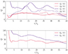 |
Fig. 2. Time-averaged profile of quality factors Qr, Qθ, Qϕ in the equatorial plane for the thick disk models with an initial β = 10 (model Q5) and β = 100 (model K3). The vertical dotted lines show the positions of the inner radius, the pressure maximum, and the outer radius of the initial torus. The horizontal line shows the level Q = 10. |
3.1. Magnetic field configuration
In the first set of models, we studied the effect of magnetic field on the QPE. We compared two thick disk models, K2 and K3 (Fig. 3). The disk in model K2 has six magnetic loops of alternate polarity, representing a more random magnetic field configuration, while model K3 has a single loop. The initial flux in each loop of model K2 is about the same and is 2.5 times smaller than the magnetic flux in model K3. We did not consider thin disks here since resolving the MRI in such disks, which is necessary to obtain a physical evolution of the disk magnetic field, requires resolutions much higher than what our computational capabilities permit.
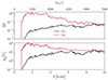 |
Fig. 3. Evolution of mass accretion rate in code units and of the jet efficiency in models K2 and K3. All values were measured at the BH horizon. The time is presented in hours, appropriate for a BH mass of 106 M⊙ (lower x axis), and in natural units of rg/c (top x axis). |
Accretion onto the BH in the case of a single loop (K3) starts sooner and reaches a higher rate than in the case of random field (K2). The main reason for this difference is that in model K2 the radial component of the magnetic field is much smaller than in K3, reducing the effective viscosity in the disk1 and increasing the accretion time. A second reason originates from reconnection in the small-scale field of model K2, which starts soon after the onset of the simulation and prevents an efficient additional buildup of magnetic field by the MRI. As a result, the disk of model K2 features a significantly lower accretion rate than the disk of model K3 despite the fact that both disks had a similar initial magnetic flux.
Another outcome of the complex magnetic field topology is a smaller magnetic flux buildup on the BH horizon, with a peak flux that is approximately one-sixth the peak flux in model K3, resulting in a lower jet efficiency in the first half of the simulation (Fig. 3). We thus conclude that the small-scale magnetic field simulations produce a smaller mass accretion rate, a lower magnetic flux through the horizon, and a low jet efficiency.
3.2. Plasma β and Kerr parameter a
To study the effect of the initial magnetization on the observational parameters, we compared the evolution of three thick disk models (K1, K3, K4) with an initial β = 1000, 100, and 10, respectively. These models have the same geometry and magnetic field configuration. The evolution of the compared parameters is shown in Fig. 4. We observed that in the more magnetized disks, accretion starts sooner, and the magnetic flux on the horizon accumulates faster and more efficiently. The mass accretion rate increases rapidly2 in the disks with β = 10 − 100, it but decreases by a factor of ten within two to six hours, becoming comparable to the less magnetized model K1. The accretion jet efficiency is higher for the highly magnetized disks and reaches a value of ∼100% in models K4 (β = 10) and K3 (β = 100), while in model K1, with β = 1000, it remains below 20%, as it has a lower initial magnetic flux in the disk, which is also converted into jet Poynting flux more slowly than for the other thick disk models.
So far we saw low accretion jet efficiency only in the multiple loops case (model K2). Another way of reproducing it is in systems with a slowly rotating BH. As shown by Lowell et al. (2024), the accretion jet efficiency ηa (in their paper it is called the EM outflow efficiency) drops when a < 0.2. To test this, we compared two thick disk models, K4 and K5, that differ only in their Kerr parameter: K4 has a fast-rotating BH (a = 0.9375) and K5 has a slower-rotating BH (a = 0.15). The results are shown in Fig. 5. The mass accretion rate is the same for both models, showing high rates in the first two hours and dropping by an order of magnitude at longer times. However, the accretion jet efficiency in the slowly rotating BH is only a few percent, making model K5 an ideal candidate to explain the lack of a variable jet in the QPEs.
3.3. Disk thickness
In all the simulations described so far, we considered ADAF-like disks without cooling. Cooling reduces the disk thickness and decreases the plasma β by lowering the gas pressure within the disk. This should have two opposite effects. On one hand, the mass accretion rate in thin disks is expected to be smaller3. On the other hand, the small β increases the viscosity parameter α in the disk and thus also the mass accretion rate. Recent work by Scepi et al. (2024) shows that the accretion rate in thin disks is higher than what has been predicted by analytical models. The situation can even be more complicated, and accretion may proceed in different channels (Jiang et al. 2019). In order to study how the disk thickness affects the observational parameters, we ran two simulations, K6, K7, with a moderately thin disks. We reduced the disk thickness to h/r = 0.3 and h/r = 0.1, respectively, by cooling the gas. It took about t = 50rg/c for the disk to reach the target scale height. We compare these models with the thick disk model K3 in the Fig. 6. As one can see, the mass accretion rate in all three simulations behave similarly despite the difference in disk thickness, and it is in a good agreement with the results obtained by Scepi et al. (2024). The jet efficiency, as expected, is smaller for the thin accretion disks.
3.4. Recurrence time
Last, in order to explain the observed recurrence time of ten hours, we required that the significant fraction of the disk mass be accreted within this time. If a significant fraction of the initial disk mass is left after ten hours, any additional mass that falls on the disk in the following cycles will result in continuous growth of the disk mass within a few orbital periods, increasing the quiescent emission and erasing the QPE signature.
In Fig. 7, we plot the current to initial disk mass ratio versus time for three different BH masses: 106 M⊙, 5 ⋅ 105 M⊙, and 105 M⊙ (respectively shown as solid, dotted, and dashed lines). We measured the disk mass as the mass of the gravitationally bounded material in the simulation defined by the criterion4
 (7)
(7)
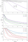 |
Fig. 7. Ratio of total disk mass to the initial disk mass versus time in the different simulations. For each model, we show the evolution of the disk mass fraction for three different BH masses: solid line (MBH = 106 M⊙), dashed line (MBH = 5 ⋅ 105 M⊙), and dotted line (MBH = 105 M⊙). |
where h = 1 + γug/ρ is the specific enthalpy, γ = 4/3 is the adiabatic index, ug is the thermal energy density, and ut is the temporal covariant component of four-velocity (equal to minus energy at infinity). Comparisons were done for all models in this work. Only models K3, K4, K5, and K6, which feature relatively highly magnetized disks, show a significant drop in disk mass within the ten-hour cycle time and a BH mass range appropriate for GSN 069. We note that in all thick and moderately thin disk models, a significant contribution to the mass loss comes from strong disk winds. This is at odds with the thin disk model (K7), in which the mass loss from winds is insignificant. Thus, despite the fact that models K7 and K3 show a similar accretion history (see Fig. 6), model K7 has a higher disk mass at the end of the cycle, making it incompatible with the observational constraint of low quiescent emission.
4. Discussion
In this work, we have explored the possibility that the QPEs observed in GSN 069 occur due to regular cycles of mass buildup in a small accretion disk around the super massive BH. We focused on two main observables: the time between outbursts and the lack of evidence for a variable jet emission. Three thick and one moderately thin highly magnetized disk models, K3–K6, can account for the required observables within some margins. Out of the three thick disks, model K4 features a significant mass loss by the end of the cycle. Models K3, K5, and K6 show similar accretion properties to model K4 but with a higher jet accretion efficiency of ηa ∼ 20% due to the larger Kerr parameter.
To estimate the disk thickness regime appropriate for our system, we compared the diffusion time at the inner parts of the disk (Ohsuga et al. 2005), tdiff ∼ 3τh/c with the accretion time ta ∼ r/vr, where vr is the radial velocity. The ratio of the two times can be formulated as
 (8)
(8)
where  is the Eddington mass accretion rate, σT is the Thomson cross section, and mp is a proton mass. Values much below unity imply that the mass is accreted faster than the energy can be dissipated, and thus the disk does not have time to puff up and remains thin. The observed peak X-ray luminosity of GSN 069 is Lx = 5 × 1042 erg s−1 (Miniutti et al. 2019) and corresponds to a mass accretion rate range of (0.4−4)ṀEdd, depending on the BH mass MBH = (106 − 105) M⊙. The associated diffusion-to-accretion time ratio falls within the value range of 0.3 − 3, suggesting that the disk should have a moderately thin to thin geometry, depending on the BH mass. We thus conclude that out of the models we examined, model K6, possibly with a relatively low Kerr parameter, is the most reasonable candidate to explain the QPEs in GSN 069.
In order to avoid emitting a significant and variable radio emission, the jets in model K6 have to accelerate freely to a distance of r ≫ c ⋅ 10 hours ∼ 104M6−1rg before they can decelerate due to interaction with the ambient medium and radiate their energy. A recurrence time of ten hours requires a combination of a disk with β ≲ 100 and a large-scale magnetic field (as can be seen in models K3–K6). These conditions could be difficult to fulfill if the disk is formed from partial disruption of a regular star, as there is no strong evidence that the magnetic field in the stellar matter has such high magnetization and regular structure. It is more likely that in this case, the initial magnetic field in the disk has a randomly distributed small-scale magnetic field, which leads to relatively slow accretion, as can be seen in model K2. The problem may be resolved if we assume that the matter forming the disk originates from a stellar wind. In stellar winds, the gas pressure drops faster than the magnetic pressure, thus the plasma β should be small. Such a scenario can be realized if we consider a binary system of two S stars with a binary period of approximately ten hours orbiting a super massive BH. Such a system typically exhibits strong stellar winds that are expected to be accreted onto the BH in the Bondi-Hoyle regime and can provide the BH with a low angular momentum5, a strongly magnetized flow of matter, and a variable on the timescale of the binary period. Circularization of this matter happens almost immediately on dynamical timescales at the Bondi radius associated with that wind. The main role of stellar winds from S stars in forming accretion disks in Galactic centers is supported by numerical simulations by Calderón et al. (2021).
In this paper, we have studied several non-stationary accretion disks. We have shown how the accretion behavior at the initial stages of the simulations is affected by the choice of initial conditions. Not only can our results be applied to the particular problem described in the paper, but they will also be useful for other studies of systems with non-stationary accretion behavior, such as gamma-ray bursts.
The viscosity depends on Maxwellian stresses Trϕ ∝ brbϕ.
The two peaks seen in the first hour in the Ṁ and ηa plots of models K4, K5 are a numerical effect originating from the onset of accretion.
According to the standard disk model (Shakura & Sunyaev 1973), thin disks accrete slower because the mass accretion rate Ṁ is proportional to the radial velocity vr, which depends on the thickness as vr = αvK(H/R)2.
Without mixing the quantity, hut is conserved along a streamline; a marginally bounded fluid element will reach infinity with h = 1 and ut = −Γ = −1, where Γ is the Lorentz factor.
This angular momentum is smaller than the orbital angular momentum by the factor (RB/Rorb)2, where RB is the Bondi radius and Rorb is the orbital radius (Wang 1981).
Acknowledgments
We thank Pavel Abolmasov, Sasha Tchekhovskoy and Matthew Green for helpful discussions. This work was supported by a grant from the Simons Foundation (00001470) to AL. This research was enabled in part by support provided by the Digital Research Alliance of Canada (alliancecan.ca).
References
- Arcodia, R., Merloni, A., Nandra, K., et al. 2021, Nature, 592, 704 [NASA ADS] [CrossRef] [Google Scholar]
- Balbus, S. A., & Hawley, J. F. 1991, ApJ, 376, 214 [Google Scholar]
- Calderón, D., Cuadra, J., Schartmann, M., Burkert, A., & Russell, C. M. P. 2021, ASP Conf. Ser., 528, 221 [Google Scholar]
- Chakraborty, J., Kara, E., Masterson, M., et al. 2021, ApJ, 921, L40 [NASA ADS] [CrossRef] [Google Scholar]
- Fishbone, L. G., & Moncrief, V. 1976, ApJ, 207, 962 [NASA ADS] [CrossRef] [Google Scholar]
- Gammie, C. F., McKinney, J. C., & Tóth, G. 2003, ApJ, 589, 444 [Google Scholar]
- Giustini, M., Miniutti, G., & Saxton, R. D. 2020, A&A, 636, L2 [NASA ADS] [CrossRef] [EDP Sciences] [Google Scholar]
- Hawley, J. F., Guan, X., & Krolik, J. H. 2011, ApJ, 738, 84 [NASA ADS] [CrossRef] [Google Scholar]
- Ingram, A., Motta, S. E., Aigrain, S., & Karastergiou, A. 2021, MNRAS, 503, 1703 [NASA ADS] [CrossRef] [Google Scholar]
- Jiang, Y.-F., Blaes, O., Stone, J. M., & Davis, S. W. 2019, ApJ, 885, 144 [NASA ADS] [CrossRef] [Google Scholar]
- Komissarov, S. S. 1999, MNRAS, 308, 1069 [Google Scholar]
- Krolik, J. H., & Linial, I. 2022, ApJ, 941, 24 [NASA ADS] [CrossRef] [Google Scholar]
- Liska, M., Hesp, C., Tchekhovskoy, A., et al. 2021, MNRAS, 507, 983 [NASA ADS] [CrossRef] [Google Scholar]
- Liska, M. T. P., Chatterjee, K., Issa, D., et al. 2022, ApJS, 263, 26 [NASA ADS] [CrossRef] [Google Scholar]
- Lowell, B., Jacquemin-Ide, J., Tchekhovskoy, A., & Duncan, A. 2024, ApJ, 960, 82 [CrossRef] [Google Scholar]
- Lu, W., & Quataert, E. 2023, MNRAS, 524, 6247 [NASA ADS] [CrossRef] [Google Scholar]
- Metzger, B. D., Stone, N. C., & Gilbaum, S. 2022, ApJ, 926, 101 [NASA ADS] [CrossRef] [Google Scholar]
- Miniutti, G., Saxton, R. D., Giustini, M., et al. 2019, Nature, 573, 381 [Google Scholar]
- Narayan, R., & Yi, I. 1995, ApJ, 452, 710 [NASA ADS] [CrossRef] [Google Scholar]
- Noble, S. C., Gammie, C. F., McKinney, J. C., & Del Zanna, L. 2006, ApJ, 641, 626 [NASA ADS] [CrossRef] [Google Scholar]
- Ohsuga, K., Mori, M., Nakamoto, T., & Mineshige, S. 2005, ApJ, 628, 368 [NASA ADS] [CrossRef] [Google Scholar]
- Pan, X., Li, S.-L., Cao, X., Miniutti, G., & Gu, M. 2022, ApJ, 928, L18 [NASA ADS] [CrossRef] [Google Scholar]
- Scepi, N., Begelman, M. C., & Dexter, J. 2024, MNRAS, 527, 1424 [Google Scholar]
- Shakura, N. I., & Sunyaev, R. A. 1973, A&A, 24, 337 [NASA ADS] [Google Scholar]
- Śniegowska, M., Grzȩdzielski, M., Czerny, B., & Janiuk, A. 2023, A&A, 672, A19 [NASA ADS] [CrossRef] [EDP Sciences] [Google Scholar]
- Suková, P., Zajaček, M., Witzany, V., & Karas, V. 2021, ApJ, 917, 43 [CrossRef] [Google Scholar]
- Tchekhovskoy, A., Narayan, R., & McKinney, J. C. 2011, MNRAS, 418, L79 [NASA ADS] [CrossRef] [Google Scholar]
- Wang, Y. M. 1981, A&A, 102, 36 [NASA ADS] [Google Scholar]
- Wang, M., Yin, J., Ma, Y., & Wu, Q. 2022, ApJ, 933, 225 [NASA ADS] [CrossRef] [Google Scholar]
All Tables
All Figures
|
Fig. 1. Initial density distribution and magnetic field configuration in the thick disk models (K1–K5). Magnetic field lines are marked by solid black lines for clockwise oriented field, and dashed white lines are used for those in the counter-clockwise oriented field. In the thin disk simulations K6, K7, we used the same single loop initial conditions. The initially thick torus evolved into a thin disk because of the cooling within the first 500 dynamical times. |
| In the text | |
|
Fig. 2. Time-averaged profile of quality factors Qr, Qθ, Qϕ in the equatorial plane for the thick disk models with an initial β = 10 (model Q5) and β = 100 (model K3). The vertical dotted lines show the positions of the inner radius, the pressure maximum, and the outer radius of the initial torus. The horizontal line shows the level Q = 10. |
| In the text | |
|
Fig. 3. Evolution of mass accretion rate in code units and of the jet efficiency in models K2 and K3. All values were measured at the BH horizon. The time is presented in hours, appropriate for a BH mass of 106 M⊙ (lower x axis), and in natural units of rg/c (top x axis). |
| In the text | |
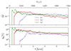 |
Fig. 4. Same as Fig. 3 but for the thick disk models K1, K3, and K4. |
| In the text | |
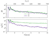 |
Fig. 5. Same as Fig. 3 but for models K4 and K5. |
| In the text | |
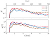 |
Fig. 6. Same as Fig. 3 but for models K3, K6, and K7. |
| In the text | |
|
Fig. 7. Ratio of total disk mass to the initial disk mass versus time in the different simulations. For each model, we show the evolution of the disk mass fraction for three different BH masses: solid line (MBH = 106 M⊙), dashed line (MBH = 5 ⋅ 105 M⊙), and dotted line (MBH = 105 M⊙). |
| In the text | |
Current usage metrics show cumulative count of Article Views (full-text article views including HTML views, PDF and ePub downloads, according to the available data) and Abstracts Views on Vision4Press platform.
Data correspond to usage on the plateform after 2015. The current usage metrics is available 48-96 hours after online publication and is updated daily on week days.
Initial download of the metrics may take a while.