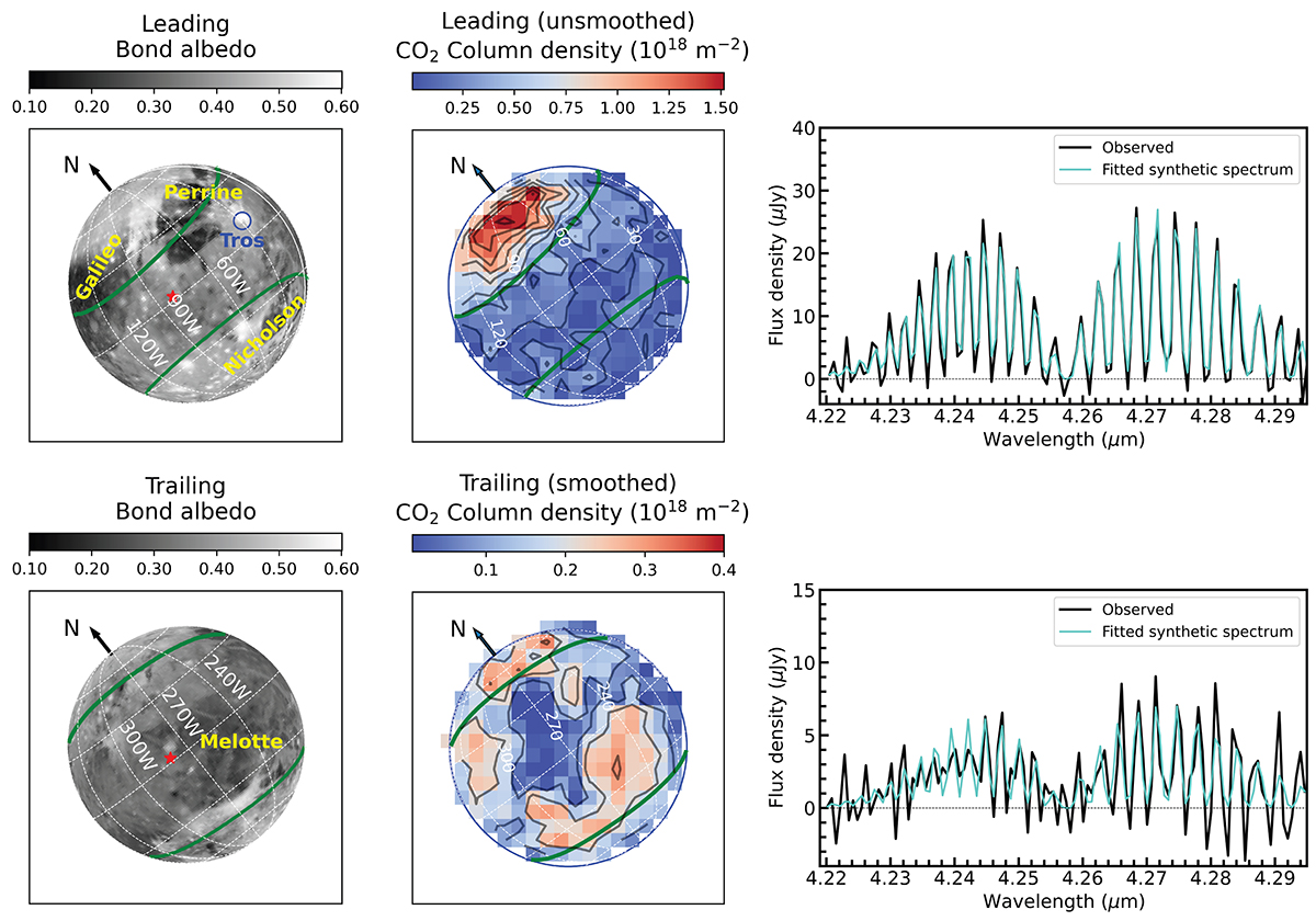
Fig. 1.
Download original image
CO2 in Ganymede’s exosphere. The top and bottom rows are for the leading and trailing sides, respectively. The left column shows Bond albedo maps derived by de Kleer et al. (2021) from Voyager-Galileo mosaic. The middle column shows line-of-sight CO2 column density maps inferred from spectral modeling (Appendices B–D). The trailing data were smoothed using a 3 × 3 boxcar filter. The color scales for the leading and trailing sides differ, and are indicated above the plots. The pixel sizes are 0.1 × 0.1″ and the PSF is ∼0.19″ (FWHM). The CO2 maximal emission in the leading hemisphere (based on central contour) is at 81°W, 51°N (∼12 h local time); correcting for the line of sight, the maximum vertical column density is at 72°W, 45°N (12.6 h local time, see Figs. 4A, O.2). The third column shows CO2 gaseous emission spectra obtained after removing the continuum emission from Ganymede’s surface, averaged over latitudes 45−90°N for leading (top), and 30−60°S for trailing (bottom). The best fit synthetic spectra are shown in cyan, with a fitted rotational temperature of 108 ± 8 K for the leading side, and a fixed rotational temperature of 105 K for the trailing side. The y scale is μJy per pixel. The green lines on the maps show the OCFBs at the time of the JWST observations (Appendix J, Duling et al. 2022). The subsolar point is shown by a red star in the Bond albedo maps.
Current usage metrics show cumulative count of Article Views (full-text article views including HTML views, PDF and ePub downloads, according to the available data) and Abstracts Views on Vision4Press platform.
Data correspond to usage on the plateform after 2015. The current usage metrics is available 48-96 hours after online publication and is updated daily on week days.
Initial download of the metrics may take a while.