| Issue |
A&A
Volume 689, September 2024
|
|
|---|---|---|
| Article Number | A349 | |
| Number of page(s) | 26 | |
| Section | Galactic structure, stellar clusters and populations | |
| DOI | https://doi.org/10.1051/0004-6361/202450971 | |
| Published online | 24 September 2024 | |
On the use of field RR Lyrae as Galactic probes
VII. Light curve templates in the LSST photometric system
1
INAF – Osservatorio Astronomico di Roma,
Via Frascati 33,
00040
Monte Porzio Catone,
Italy
2
Instituto de Astrofísica de Canarias,
Calle Via Lactea s/n,
38205
La Laguna,
Tenerife,
Spain
3
Departamento de Astrofísica, Universidad de La Laguna, Avenida Astrofísico Francisco Sánchez,
s/n, 38200 San Cristóbal de La Laguna,
Tenerife,
Spain
4
INAF – Osservatorio Astronomico di Capodimonte,
Salita Moiariello 16,
80131
Napoli,
Italy
5
Department of Physics and Astronomy, Vanderbilt University,
Nashville,
TN
37240,
USA
6
Konkoly Observatory, HUN-REN Research Centre for Astronomy and Earth Sciences, MTA Centre of Excellence,
1121 Konkoly Thege Miklós út 15–17,
Budapest,
Hungary
7
ELTE Eötvös Loránd University, Institute of Physics,
1117 Pázmány Péter sétány 1/a,
Budapest,
Hungary
Received:
3
June
2024
Accepted:
15
July
2024
Abstract
Context. The Vera C. Rubin Observatory will start operations in 2025. During its first two years, too few visits per target per band will be available, meaning that the mean magnitude measurements of variable stars will not be precise and thus standard candles such as RR Lyrae (RRL) will not be usable. Light curve templates (LCTs) can be adopted to estimate the mean magnitude of a variable star with a few magnitude measurements, provided that their period (plus the amplitude and reference epoch, depending on how the LCT is applied) is known. The LSST will provide precise RRL periods within the first six months, enabling exploitation of RRLs if LCTs are available.
Aims. We aim to build LCTs in the LSST bands to enhance the early science with LSST. Using them will provide a one- to two-year advantage with respect to the classical approach concerning distance measurements.
Methods. We collected grί-band data from the ZTF survey and z-band data from DECam to build the LCTs of RRLs. We also adopted synthetic grίz band data in the LSST system from pulsation models, plus SDSS, Gaia and OGLE photometry, inspecting the light amplitude ratios in different photometric systems to provide useful conversions to apply the LCTs.
Results. We have built LCTs of RRLs in the grίz bands of the LSST photometric system; for the z band, we could build only fun damental mode RRL LCTs. We quantitatively demonstrated that LCTs built with ZTF and DECam data can be adopted on the LSST photometric system. The LCTs will decrease the uncertainty on distance estimates of RRLs by a factor of at least two with respect to a simple average of the available measurements. Finally, within our tests, we have found a brand new behavior of amplitude ratios in the Large Magellanic Cloud.
Key words: methods: data analysis / stars: distances / stars: variables: RR Lyrae
Corresponding author; This email address is being protected from spambots. You need JavaScript enabled to view it.
© The Authors 2024
 Open Access article, published by EDP Sciences, under the terms of the Creative Commons Attribution License (https://creativecommons.org/licenses/by/4.0), which permits unrestricted use, distribution, and reproduction in any medium, provided the original work is properly cited.
This article is published in open access under the Subscribe to Open model. This email address is being protected from spambots. You need JavaScript enabled to view it. to support open access publication.
1 Introduction
The Vera C. Rubin Observatory will see first light at the beginning of 2025, and for ten years, it will carry on the Legacy Survey of Space and Time (LSST), surveying the entire southern sky in six passbands (ugrizy). The synergy of the wide field camera (3.5 square degrees) and the large primary mirror (8.4 m diameter) will be the keys for the unprecedented efficiency of the so-called Wide-Fast-Deep (WFD) survey within LSST. The WFD will deliver the most extended set of light curves for variable stars in terms of the following combined properties: (I) epoch extension (10 years); (II) sky area (18 000 deg2); (III) number of phase points (more than 800 in total); (IV) number of passbands (six, from u to y); and (V) depth: r ~ 24.03 (26.90) mag with 5σ signal-to-noise, for the single exposure (10-year co-added image). The WFD is conceived to be a complement of the Gaia mission (Gaia Collaboration 2016) in the inner bulge and in the outer halo concerning not only variability but also astrometry.
The RR Lyrae (RRLs) are old low-mass core-Helium-burning stars on the horizontal branch pulsating regularly with periods of 0.2–1.4 days (Soszyński et al. 2019; Braga et al. 2021). The RRLs are present in every component of the Milky Way – globular clusters, the halo, bulge, and thick disk – and, recently, several thin disk RRLs were also found (Prudil et al. 2020; Matsunaga et al. 2022). The RRLs obey to tight period-luminosity (PL) relations at effective wavelengths ranging from ~600 nm to ~4500 nm, thus including all passbands between, for example, R (or r) and M (or [4.5] in the Wide-field Infrared Survey Explorer (WISE) system; Longmore et al. 1986; Catelan et al. 2004; Madore et al. 2013; Braga et al. 2015). This makes them reliable old-age standard candles, and they are therefore a complement to the distance estimates of the young and more luminous Classical Cepheids (Leavitt 1908; Madore & Freedman 1991; Skowron et al. 2019). The RRLs are also metallicity probes since they obey P–[Fe/H]-ϕ3ı relations, where ϕ31 is a parameter derived from the Fourier coefficient of the fit of the light curve (Jurcsik & Kovacs 1996; Mullen et al. 2022; Kovacs & Jurcsik 2023). Metallicity has an important role since it also affects PLs. Therefore, the period–luminosity–metallicity (PLZ) relations can also be used as iron abundance diagnostics once the distance is known (Martínez-Vázquez et al. 2016; Braga et al. 2016). Period-Wesenheit (PW) relations and period-Wesenheit-metallicity (PWZ) relations, where the Wesenheit is a pseudo-magnitude that is reddening-free by construction (Madore 1982), were used as distance indicators, too. It is worth noting that some combination of magnitudes, especially toward bluer passbands, give metallicity-insensitive PWZs, as verified both theoretically and empirically (Marconi et al. 2015, 2022; Ngeow et al. 2022; Narloch et al. 2024, Accepted for publication in A&A) Thanks to all of these properties and being strictly old (≳9 Gyr; however, recent studies theorize that a minority of metal-rich thin disk RRLs could be young, as they are the outcome of a merger Bobrick et al. 2024), they can be used as tracers of the earliest stages of Galactic evolution (Fiorentino et al. 2015; Iorio & Belokurov 2021).
To fully exploit RRLs as probes of Galactic evolution, it is mandatory to estimate accurate mean magnitudes (<ma𝑔>), as in turn they provide individual distance estimates by means of the PL relations. Being variable stars, a <ma𝑔> estimate requires a good sampling of the pulsation cycle to properly model the light curve. However, as shown by Jones et al. (1996) and Braga et al. (2019), light curve templates (LCTs) can be adopted to estimate accurate <ma𝑔> that have only one observed phase point (provided that the period, light amplitude [Ampl], and the reference epoch are well constrained). The LCTs are, in short, analytical functions (or gridded points) that reproduce the typical shape of the light curve of a variable star within a specific range of periods and Ampl, pulsating in a specific mode. The RRLs pulsate either in the fundamental (F) or in the first overtone (FO) mode, or both simultaneously – the so-called double-mode (DM). Empirical evidence for the existence of second overtone (SO) RRLs is not clear (Kiss et al. 1999; Rodríguez et al. 2003), and SO RRLs are not supported theoretically by pulsation models (Stothers 1987). Therefore, we ignore SO RRLs in this work. We also ignore DMs because (1) additional factors come into play (e.g., the difference in phase and the Ampl ratio between the two modes) and (2), concerning PLs and distance estimates, DMs were either discarded or treated as FO RRLs since the dominating mode is generally the FO. To sum up, we focus only on F and FO LCTs.
The empirical classification of RRLs into RRa, RRb, and RRc based on the shape of their light curves dates back to Bailey (1902). Schwarzschild (1940) associated the RRa and RRb stars (sawtooth-shaped light curves, later unified into the RRab class) with the F mode and the RRc stars (sinusoidal light curves) with the FO mode. The pulsation mode is therefore the most important parameter to consider for LCTs. However, RRLs pulsating in the same mode can have significantly different light curve shapes, and the most reliable parameter to separate the different morphological classes of light curves is the pulsation period (Inno et al. 2015; Braga et al. 2019).
The main aim for which the LCTs in this work are conceived is to enhance the science performed with LSST early data. By “LSST early data” we mean both the commissioning data, realtime calibrated images, and Data Releases 1 and 2 (6 and 12 months of data, respectively). Observations from DR1, for example, will allow for a period estimate with precision better than 0.05% for typical RRL periods (Di Criscienzo et al. 2023) but also with uncertainties on <ma𝑔> up to 0.1–0.2 mag. This will translate into a distance uncertainty of up to 20%, which is too large for any galactic archaeology analysis with RRLs. Using the LCTs from this work will mean having an advantage of one to two years compared with a more classical approach concerning the distance determination of RRLs. This is going to be particularly interesting in the bulge and in the outer halo, where LSST will discover hundreds of thousands of new RRLs. We point out that the LCTs by Sesar et al. (2010, hereinafter, S10), although they cover SDSS ugriz passbands, are not fit for our purpose, and this is the reason why we decided that new LCTs are necessary.
The paper is structured as follows. In Section 2, we present the dataset used to build the LCTs; the procedure adopted to build the LCTS is explained in Section 3. We discuss the accuracy of our LCTs and how to use them in Section 4 and report our conclusions in Section 5. We added three sections in the Appendix to discuss the shape of the LCTs, the comparison with S10 LCTs, and the light amplitude ratios.
2 Dataset
In general, LCTs are built starting from normalized and overlapped light curves observed in a given passband. In our case, this is not possible since Rubin Observatory has not started its operations yet, meaning that there is no existing observed data in the ugrizyLSST (ugrizyL, in short) photometric system.
Therefore, as a database to build the LCTs, we decided to adopt light curves collected by other instruments, with passbands as similar as possible to the ugrizyL photometric system. The two empirical datasets that we have selected are: (1) Zwicky Transient Facility (ZTF, Bellm et al. 2019; Masci et al. 2019) light curves of RRLs in the 𝑔riZTF bands (𝑔riZ, in short), selected from our catalog of ~286000 RRLs, mostly based on Gaia DR2+EDR3, plus other surveys (Fabrizio et al. 2019, 2021); (2) The Dark Energy Camera (DECAM, DePoy et al. 2008) survey of the Galactic bulge by Saha et al. (2019) in the u𝑔rizDECam (u𝑔rizD, in short).
A critical question arises as to whether we can really adopt ZTF and DECam passbands to derive LCTs that can be used with LSST data. A detailed answer to this question is be given in Section 3.6.
2.1 ZTF
The extremely large 47ºfield of view of ZTF allowed this instrument to survey the sky very quickly, collecting hundreds of 𝑔rZ-band plus tens of iZ-band phase points per target. From now on, we use the suffix Z to refer to the ZTF photometric system. Nonsuffixed passband names are used when referring to the LCTs and to passbands in general. As a starting sample, we adopted our catalog of RRLs based on Gaia DR2+EDR3 and other surveys, such as Catalina, ASASSN, and PanSTARRS (Fabrizio et al. 2019, 2021, and references therein). By using Gaia EDR3 coordinates for this catalog, we queried the ZTF DR17 database and retrieved a catalog of 35434/29510/9949 𝑔Z/rZ/iZ light curves. To keep only the best sampled light curves to build the LCTs, we rejected all the light curves with a value of ngoodobsrel (number of epochs within the current data release, without photometric quality issues) larger or equal than 80.
After this cut, the catalog narrowed down to 24 925 RRLs in total. We have downloaded 23 849/19 146/2192 𝑔Z /rZ /iZ light curves for these objects. The 𝑔Z /rZ /iZ light curves have, on average, 303/499/88 phase points. These numbers are the result of the rejection – already in the query step – of all the observations with catflags ≥32768 (i.e., measurements for which moon illumination or clouds might have hampered the photometric quality).
2.2 DECam
Unfortunately, the ZTF survey did not collect images with pass-bands redder than i. Nonetheless, for our purpose, it is crucial to push our LCTs at longer wavelengths, because LSST will acquire images also in z and y. These are the most important filters to investigate the bulge of the Milky way, since longer wavelengths are less affected by the extreme reddening in that region. Moreover, the PL relations have a higher slope (meaning that they are more precise distance indicators) at redder passbands.
For this reason, we complemented the ZTF sample described above with DECam time series of RRLs in the bulge collected by Saha et al. (2019). They acquired tens of images in each of the ugrizD passbands (where the D suffix refers to the DECam photometric system) and detected 474 RRab. Unfortunately, their sample does not include RRc since they did not search for them. This means that we could not obtain zD-band LCTs for this pulsation mode. We also point out that we will not use uD-band data to build u-band LCTs. First of all, the u band is less important for distance determination, because the PL is flat and has a high dispersion at short wavelengths. Secondly, the steepness of the u-band light curve makes it difficult to provide good fits with the available sampling.
3 Template building
For the 𝑔ri LCTs, we adopted only the ZTF data for three reasons. First, the contribution from DECam would be tiny. For the 𝑔r bands, ZTF light curves have approximately ten times more phase points, and the number of RRLs is about two orders of magnitude larger. For the i band, the ZTF RRL sample is around five times larger than the DECam one, and each light curve has around twice as many phase points. Overall, the number of phase points in ZTF is three (one) orders of magnitude larger than the DECam sample, in the 𝑔r (i) bands, respectively. Second, when possible, we prefer not to merge datasets from different instruments in order to avoid transformations between photometric systems that would only introduce noise and, consequently, an intrinsic dispersion in the LCTs. Third, the ZTF and DECam catalogs of RRLs are qualitatively different since they provide light curves of halo and bulge RRLs, respectively, and it is well-known that the former are more metal-poor than the latter ([Fe/H] − 1.51+0.41 compared to ~−1.0 Fabrizio et al. 2021; Walker & Terndrup 1991). Since the shape of the light curve is notoriously dependent on the iron abundance at all wavelengths (Jurcsik & Kovacs 1996; Mullen et al. 2022), we prefer not to merge the two datasets. Nonetheless, we note that we have compared the amplitudes of the ZTF and DECam light curves and found no significant difference (see Appendix D) but the parameter that really depends on metallicity is ϕ31 (Jurcsik & Kovacs 1996). One might argue that metallicity should be taken more into account when building LCTs but there are two reasons for which we do not provide different LCTs for different ranges of metallicities, for example. First of all, only a tiny fraction (~1%) of our RRLs has an iron abundance estimate. This would mean to sacrifice the excellent sampling that we have for the 𝑔 and r bands and not having enough statistics to derive any i and z LCT. Secondly, our main aim is not to provide a complete taxonomy of the light curves of RRLs, but providing models that can be used to estimate <ma𝑔> and distances of RRLs that will be, mostly, new discoveries from LSST, and for which no estimate of [Fe/H] will be available, making it also impossible to use this information, even by having LCTs separated in [Fe/H] bins.
To build the LCTs, one has to 91) fold all the light curves by the proper period and adopt the same reference epoch (T0) for the zero phase; (2) normalize the light curves; (3) merge all the normalized light curves in a given band and period bin into a single cumulated and normalized light curve (CNLCV); (4) derive an analytic fit of the CNLCV. This will be the analytic form of the LCT.
3.1 Phasing of the light curves
As already discussed in Braga et al. (2019, 2021) we usually adopted, as a reference epoch for our LCTs, the epoch of <ma𝑔> on the rising branch of the V-band light curve  , introduced by Inno et al. (2015), instead of the more commonly used epoch of maximum light (Tmax). In fact, Inno et al. (2015) and Braga et al. (2021) demonstrated that
  provides a better anchor epoch with respect to Tmax, because the CNLCVs have a smaller dispersion (see Figs. 2 and 8 in Braga et al. 2021). We point out that the LCTs provided in the quoted papers (JHK-band light curves and radial velocity curve templates) were anchored to a reference epoch in the V band because they are meant to be applied on scarcely sampled NIR or radial-velocity time series, by adopting ephemerides from well-sampled V-band data. They followed this approach because V-band surveys are larger and better sampled than any NIR and radial-velocity survey, and usually precede them in time.
However, the 𝑔riz LCTs that we provide in this paper are meant to be used in a different way. They are not applied to poorly sampled light curves of known variables when a well-sampled V-band light curve is already available. Instead, they are applied to candidate RRLs for which the early LSST time series provides only an estimate of the pulsation period and a <ma𝑔> to be improved with the LCT itself. This means for the LCTs that we provide, the best phase anchors are  for the 𝑔riz LCTs respectively.
To estimate Tris for the ZTF 𝑔riZ light curves, we followed a two-step method: 1) After folding the light curves with the proper period and shifting them to a preliminary and arbitrary reference epoch (T0=0), we fitted the light curves with Fourier series. We adopted a dynamical selection of the Fourier degree, starting from a base of 3/6 for RRc/RRab stars and increasing by one, up to a maximum degree of 12. At each step,  (the χ2 for the nth-degree fit) and
  , for the n-th and n + 1-th degree fits are derived and their ratio
  is derived. The larger is
  , and the less significant is the improvement of the fit when increasing the degree. We have set a 0.99 thresh-old
  so that, when
  was smaller than that, we increased n. When
  , we stopped the iteration and adopted n as the degree of our best-fitting model. We point out that we did not apply any sigma clipping of the phase points because this would invalidate the χ2 comparison, since the residuals would be calculated on different datasets. The χ2 comparison might seem biased with a very large value of the threshold fraction and favoring too high degrees. However, to properly calculate Tris, it is important that the rising branch is very well fitted and, especially for RRab this usually requires high Fourier degrees. This is why we had set a quite high cap on the Fourier series degree (12) and selected carefully the training sample of the neural network (NN; see Section 3.2). This was done in order to be sure that the estimate of Tris was not affected by features on the rising branch (e.g., the hump before the maximum). We point out that this iterative method for the degree selection, was selected over others (e.g., the Bayesian Information Criterion) for at least two reasons: (1) the direct control over the χ2 ratio; (2) its similarity with the reliable method adopted within the Gaia Collaboration (S. Leccia, private communication). (3) By adopting the model fit, we derived the <ma𝑔> of the star and, by searching its intersection with the rising branch fit (see Appendix C.1 in Braga et al. 2021), we derived Tris. Having an estimate of Trisfor each light curve, the time series were rephased by adopting this new reference epoch, and the folded light curves were refitted, obtaining the final Fourier series model. The latter provided Ampl and <ma𝑔>, integrated over an arbitrary flux scale.
For the zD-band light curves, we followed a qualitatively identical algorithm to phase the light curves. The only difference is that we performed fits adopting both Fourier series and PLOESS models (Braga et al. 2016, and references therein), and selected the best-looking one, with a visual inspection. This approach was necessary because the DECam light curves are not as well sampled as the ZTF ones and the Fourier fit often failed, especially when large gaps are present.
Predictors used for the neural network.
3.2 Selection of the light curves
Not all the light curves in our database are suitable to build the LCTs. Therefore, we added a selection algorithm to keep only the best light curves.
The ZTF dataset is so large that it was not possible to visually inspect all the light curves. Therefore, we adopted an NN to perform the selection. First, we selected a training sample of 681 𝑔ri light curves, we visually inspected all the light curves and manually flagged the light curves that should be kept/rejected for the template building. We tested several combinations of predictors and NN architectures and found that the best solution is to adopt, as predictors, the parameters in Table 1 and an NN architecture with two hidden layers, each with 14 perceptrons.
The NN was built by using the Python package sklearn and, more precisely, the MLPClassifier, with a maximum iteration number of 40000, an optimization tolerance of 0.0001, a ‘tanh’ function for the activation and the default ‘adam’ value for the solver parameter. We tested the accuracy of the NN and obtained a train/test converging ratio of 0.91/0.88.
The NN provided us a predictor that we have applied to the entire dataset of ZTF light curves, obtaining a True/False rejection flag for each light curve. After this task, the sample of light curves to be kept to build the LCTs was 14829/12239/1243 for the 𝑔Z/rZ/iZ bands, respectively. We have visually inspected a small sample of the light curves flagged by the NN, and found that a very high fraction of the selections were performed correctly. Therefore, we were satisfied with the adopted NN and did not build an NN for each filter.
We did not adopt a machine learning algorithm for the DECam data because the sample is too small, and because the visual inspection – that would be required anyway to set the training sample – does not take too much time on such a limited sample. After the fitting, we rejected all the light curves that are not suitable to build the LCTs, meaning those with less than 14 phase points, those for which a reliable measure of Ampl is not available and those with a large dispersion around the fit of the light curve. We end up with 217 zD-band light curves of RRab with 14-to-86 phase points, covering a period range between 0.356 and 0.822 days (see Fig. 1).
Tables A.1 and 2 report, for the ZTF and DECam databases, the coordinates and pulsation properties; Table A.1 also reports the light curve fitting statistics needed to run the selection algorithm described above. Figure 1 displays the distribution in period (left panels) and Bailey diagram (right panels) of the final sample of stars. One can see that all of these datasets are made mostly by Oosterhoff I (OoI) RRLs and host a smaller fraction of Oosterhoff II (OoII) RRLs, where OoI and OoII RRLs are typically associated to metal-rich/metal-poor Globular Clusters of the Milky Way (Oosterhoff 1939). We note that, for our zD-band dataset, OoII RRLs seem to make up an even smaller fraction of the total number of RRLs – as expected due to the higher average metallicity of bulge RRLs with respect to halo RRLs – but we do not have enough statistics to assert this on a quantitative basis.
We conclude this section by pointing out that, for each period bin (see Section 3.3), we kept out of the selection, three RRLs that would be suitable to build the LCTs. These will be used as independent data for the validation of the LCTs themselves (see Section 4).
Pulsation and fitting properties of the DECam z light curves of RRLs.
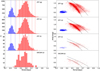 |
Fig. 1 Period distributions and Bailey diagrams of our ZTF and DECAM RRLs. Left panels, from top to bottom: period distribution of the RRLs adopted to build the templates in the 𝑔ZrZiZzD bands. The RRab are displayed in red and RRc in blue. The red and blue dashed lines display the period thresholds of the LCTs derived in this work, for RRab and RRc, respectively. Right panels: same as left but for the Bailey diagram (period versus Ampl). Dashed black lines display the loci of the Oosterhoff tracks derived by Fabrizio et al. (2019) and transformed into the 𝑔ZrZiZzD bands using the ratios derived in Appendix D. |
3.3 Period binning
The basic assumption for the LCTs is that different stars of the same variability class, same pulsation mode and with similar physical properties should have similar light-curve shapes. Recent studies demonstrated that stars with different pulsation properties might have very similar light curves (Jurcsik & Juhász 2022), but these are a minor fraction and the quoted assumption is still valid when dealing with large datasets, which is the purpose of LCTs in this work.
Since the physical properties are not easily measurable, one should adopt one (or more) easily measurable parameters to group RRLs in template bins inside which all the variables have a similar shape of the light curve. We adopted two parameters: (1) the pulsation mode and (2) the pulsation period. The former is quite obvious and provides a dichothomic separation of light curves (almost sinusoidal for RRc and sawtooth-like for RRab). The latter should be better justified, and we do this in the following paragraphs.
In principle, the shape of the light curves of RRab and RRc depends on their physical properties (mass, temperature, chemical composition…) but these properties are not easy to measure. Luckily, the pulsation period (P) is an easily measurable quantity and is connected to the main physical properties of the stars by the pulsation relations (van Albada & Baker 1971; Marconi et al. 2015), of the form
 (1)
(1)
and
 (2)
(2)
As a consequence, the properties of RRLs scale with P. This is quite straightforward for <ma𝑔>, as it appears from the Period-Luminosity relations (PLs, Longmore et al. 1986; Bono et al. 2003; Madore et al. 2013); this is also true (although less clear due to nonlinear effects) for Ampl, as one can see in a Bailey diagram (Bailey 1902). We point out that P has several advantages with respect to the amplitude, for example, which was adopted for RRLs by Jones et al. (1996): First, it is the easiest parameter to measure. With LSST multi-band data, period measurements will be precise up to 1e-5 days with only six months of data for half of the stars with 𝑔 ~23.0 and for up to 70% of the stars with 𝑔 ~ 21.0 (VanderPlas & Ivezić 2015; Di Criscienzo et al. 2023, Di Criscienzo, private communication). Second, RRLs showing secondary modulations (Blazhko and double-mode) have a precise measure of the period, while the same is not true for the amplitude. Last, P, as Ampl, is independent of distance and reddening, which are not always easy to estimate.
This is the reason why a crucial operation is the selection of the thresholds of period bins: all the normalized light curves (NLCVs) of RRLs with a period inside a given bin should be merged, providing one CNLCV per bin, per band. Thus, the selection of the thresholds of the period bins is the key to separate properly the different light curve shapes.
Figure 1 displays the period distribution of the RRab and RRc that we will use to build the LCTs. Due to the different number of RRLs within the datasets in different passbands, we had to adopt different criteria to split the bins.
We started by selecting the bins for the RRab stars. The period range covered by RRLs for all the bands is 0.35–0.83. There are a few RRLs with period >0.83 days, but their number is small and we do not build any template if there are less than three RRLs in a bin.
After several tests and deriving LCTs for different bin sizes, we decided to divide this period range into bins of 0.06 days for the ZTF (griz) database, with only two exceptions: 1) due to the very large number of variables between 0.59 and 0.65 days, we splitted this bin in two for the grz data; 2) since, for the iz band, we have fewer data, we merged the two bins 0.71–0.77 and 0.77–0.83 into one larger bin, to have sufficient statistics and derive a reliable LCT.
The bins for the 𝓏 band LCTs, however, must be wider, since the DECam dataset is considerably smaller (around 12 000 phase points in total, which is a factor of 400 smaller than the ZTF 𝑔z and rz samples). Therefore, in this case, we selected a bin width of 0.12, which is twice as large as that of the griz bands.
For the RRc stars, which cover around 0.17 days in pulsation periods, we have more than 1/1.5 million phase points for the 𝑔z/rz bands, respectively, and almost 40000 for the iz band. We have tried several different bin sizes but the optimal solution is to adopt two bins of 0.08 days and a longer-period bin of 0.04 days for each band. Although smaller bins would be possible thanks to the large number of phase points, these would be useless since LCTs would be almost indistinguishable between these smaller bins. Indeed, the LCTs for the mid- and long-period RRc are very similar, apart from the hump at phase 0.05–0.10 in the iz-band. Therefore, we performed some tests by shifting the bins by steps of 0.01 days, to check how the LCTs changed by moving the thresholds. The tests revealed that despite the small sample size of the longest bin, the difference in shape is solid and real. In fact, when decreasing the low-period threshold of the long-period bin, the hump becomes less and less evident. Therefore, we provide the three LCTs as described.
3.4 Normalization and cumulation of the light curves
Since the LCTs are provided as normalized curves, with mean 0 and amplitude 1, we have normalized the folded time series of all the RRLs in all the bins, by subtracting < ma𝑔 > from all the measured magnitudes of each phase point, and then dividing them by the light amplitude. This process provided us the normalized light curves (NLCVs).
After this operation we collected, for each passband and each period bin, the phase points of all the NLCVs within that bin. The result is a single light curve that is the cumulation of all the NLCVs in the same band, with similar periods and therefore with similar shapes. This is what we call the cumulated and normalized light curve (CNLCV). Table A.2 displays the number of phase points and of RRLs for each CNLCV.
We note that we did not generate any CNLCV (meaning that we did not derive any template) for bins with less than three light curves because such a limited statistics cannot really guarantee that there is no true difference in the shape for a period range with such little data.
3.5 Fitting
Finally, we derived the analytical form of the LCTs by fitting, with a Fourier Series, the CNLCVs. However, we noted that a simple fit on all the phase points is not the best solution because it often generates models that are too smooth and for which the typical features of RRL light curves at that period are lost. This happens for any degree that is adopted for the Fourier series. Therefore, we have built 2D histograms in the phase-Nmag (normalized magnitude) plane, on a nx × ny grid, from a minimum of 90×90 to a maximum of 500 × 500 cells, slicing the [0,1] phase range and the [1,−1] Nmag range. nx and ny were individually selected for each of the CNLCVs. We point out that nx may be different from ny. We counted the number of phase points in each cell (Nij, with i and j running over nx and ny) and generated a density plot. At first, we tried to simply take the densest cell for each vertical slice (that is, at each phase) and then perform a fit on these points. However, this technique provides inaccurate models, with nonrealistic ripples.
Therefore, we decided to take, for each of the nx phases, an arbitrary number (between four and ten, selected individually for each CNLCV) of the densest cells (ncell) of the vertical slice, and calculated the weighted average of their Nmag. As weights for each of the ncell, we adopted Nij, so that the densest cells have more weight in the average. In this way, we obtain a number nx of average magnitudes (< Nma𝑔i >), each associated to a specific phase. Finally, we fitted these points with a Fourier series and obtained the definitive, analytical form of the LCTs. The density plot and the fit of a sample LCT is displayed in Fig. 2. We note that, for all the fits, the degree of the Fourier series is dynamically selected by setting a  of 0.995-to-0.999, and a maximum Fourier-series degree of 40.
Table A.2 lists the Fourier series coefficients representing the analytical form of the LCTs and the statistics behind the template building. The figures showing the analytic forms of the templates are displayed in Appendix B.
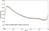 |
Fig. 2 Density plot of a CNLCV (𝑔 band, RRab, period bin [0.35–0.41 days]). Darker cells are the most dense. The red crosses display the average of the four highest-density cells at each phase. The green, solid line shows the Fourier fit of these average points. |
3.6 Applicability to LSST photometric system
To build the LCTs, we have used data from two different photometric systems (DECam and ZTF), neither of which is that of LSST. As shown by Table 3, the difference of both the effective wavelength (λeff) and the effective width (Weff) of the same passband in two different photometric systems can range from a few tens of to a few hundreds of Å, especially in the 𝓏 band. Therefore, we have to check whether and how the reliability of our LCTs is affected when used on LSST data.
For variable stars, there are three main properties that can be affected when one considers the differences between two photometric systems: (1) < ma𝑔 >; (2) Ampl; (3) the shape of the light curve.
Characteristic wavelengths of the DECam, ZTF, and LSST passbands.
3.6.1 Mean magnitude
Luckily, when working with LCTs, one does not need to know < ma𝑔 > in advance because the template can either be fitted leaving a free magnitude offset, or it can be anchored to a phase point, if the ephemerides are known. In both cases, < ma𝑔 > is an output and not an input of the process. Therefore, we can ignore the effect of < ma𝑔 > caused by adopting different photometric systems. Nonetheless, we performed a simple test by fitting the DECam light curves with 𝑔ri LCTs derived from ZTF. The offset in < ma𝑔 > is generally smaller than 0.01 mag, and this is also the case for RRab with a high amplitude, which has the sharpest and most asymmetrical light curves and is therefore the least easy to fit, at least with respect to RRab with smaller amplitudes and, in general, to RRc.
3.6.2 Light amplitudes
When using the LCTs, one has to rescale the normalized amplitude of the LCT to the real (or the expected) Ampl of the observed variable. There are several methods to set the value of Ampl: (1) to leave Ampl as a free parameter in the fit; (2) to set a fixed value of Ampl based, for example, on the Ooster-hoff sequence relation (log P versus Ampl) in the Bailey diagram (Cacciari et al. 2005; Fabrizio et al. 2021), taking advantage of the knowledge of the pulsation period; (3) in the case that the LCT is applied to an RRL with known pulsation properties (including Ampl(X) in a given X passband) from a former survey, one can adopt Ampl(X). Concerning case (1), Ampl is an output of the process and not an input, meaning that one can use the LCTs on LSST data without any concern. We note well that, when the LCT is applied to Rubin Observatory data (which would be the main use of LCTs provided in this paper) one will have to adopt a value of Ampl in the LSST photometric system for a proper rescaling. In cases (2) and (3), Ampl is an input and it should be converted into Ampl(xL), where xL is the LSST passband to which the template must be applied. The calculation and discussion on the amplitude ratios is extensive and detailed and would break the current discussion on how to adapt the LCTs to the LSST photometric system. Therefore, we present it in Appendix D.
3.6.3 Light curve shape
Unfortunately, concerning the shape of the light curves, we cannot provide any quantitative estimate of differences between the LSST, DECam and ZTF passbands. In fact, the DECam light curves have too few phase point to derive the fit coefficients. Furthermore, we cannot even compare the synthetic light curves that we used for the amplitude ratios. In fact, while these can provide accurate estimates of < ma𝑔 > and Ampl, they display some features (e.g., humps before the maximum) that are not observed in real-life photometric data. This means that any comparison with, for example, Fourier series coefficients or principal components, would not be reliable when applied to empirical data. Even more importantly, since LCTs are meant to be used on a small number of observed phase points and the final goals are (1) to help with the separation between RRc and RRab and (2) to get a < ma𝑔 > estimate, tiny differences in the shape lead to errors that are smaller than the intrinsic uncertainty of the LCTs and the propagation due to the amplitude rescaling. Also the idea of converting directly the observed light curves between the different datasets, although feasible in principle, has to be discarded: for a computationally heavier approach, we could introduce uncertainties due to the intrinsic spread of the conversion equations and to their limitations in color range and evolutionary stage. Moreover, even in the case that the shape of the light curves is actually improved, the change would be tiny and, as already explained, the improvement would be smaller than the intrinsic uncertainty of the LCTs.
4 Validation
After deriving the analytical form of the LCTs, we have tested their performance. As anticipated in Section 3.2, we left a few variables (three for each period bin in every passband) out of the database that was used to build the LCTs. We used these RRLs to validate the LCTs with independent data. To perform our validation, we considered realistic future scenarios in which one will use RRLs for the investigation of Galactic structure and formation. In these cases, LCTs could be used to obtain accurate < ma𝑔 > estimates and, in turn, distances, of RRLs during the commissioning or the first couple of years of observations with LSST. This is, as already mentioned in Section 1, our aim in delivering these LCTs: to enhance early science with LSST, having more precise distances for these important old population tracers.
Using LSST data, our LCTs can be used to improve the estimate of mean magnitudes, adopting two different techniques: (1) LCT anchoring on a single (or more) phase points, when the period, reference epoch and light amplitude in a given passband are known; (2) LCT fitting of the light curve, in the case that the reference epoch is not known and a few phase points are available in a given passband. Case (2) splits in two: (2a) fixed amplitude in the fitting process (minimum three phase points required, plus the pulsation period and Ampl); (2b) amplitude as a free parameter in the fitting process (minimum four phase points required, plus the pulsation period). In the following sections, we discuss our tests using these three techniques.
4.1 Single point anchoring validation
Applying LCTs on single phase points of RRLs with well-known pulsation properties is the original purpose of LCTs of RRLs (Jones et al. 1996) and variable stars, in general. The LCTs provided in this work are aimed to extract as much information as possible from LSST early data, including that narrow window (1 or 2 months from the beginning of the survey) when only one phase point per band per target will be available. In this case, one can apply the LCTs only to variables for which both the period, reference epoch and Ampl are known, otherwise there would be not enough information to anchor the LCT on one point. A practical example of relevant scientific interest is that of RRLs found by OGLE in the bulge (Soszymki et al. 2019). In fact, for these OGLE RRLs, we have detailed information but only in the I and V bands. However, obtaining < ma𝑔 > in more passbands, means to be able to use different PLs and PW. This approach allows both validation of the results obtained by OGLE itself and improvement of them thanks to, for example, the higher slope and smaller dispersion of the PL(z), or the insensitiveness of PW(r,𝑔 – r) on metallicity (Marconi et al. 2022). Moreover, having < ma𝑔 > in three to four passbands allows one to follow the extinction law on a wider range of wavelengths if one is interested in doing so.
A conservative estimate based (1) on the assumption of a saturation limit of 16 mag in the iLSST band (LSST Science Collaboration 2009); (2) a maximum iDECam – I color of 0.3 mag, verified on the subsample of OGLE RRLs matching those in (Saha et al. 2019), assuming iDECam ≈ iLSST; (3) ~0.45 mag as half of the maximum Ampl(i) (see Figure 1), tells us that at least 41 000 RRLs with known pulsation properties from OGLE (~60% of the total sample of ~68 000) will not saturate in the LSST images. Unfortunately, the overlap between the OGLE RRLs and ZTF RRLs is poor and there are not enough RRLs to validate the gri LCTs with the quoted sample. On the other hand, OGLE and DECam bulge RRLs overlap almost completely, meaning that, for the z-band LCTs, we can simulate the quoted scientific case.
In the following, we describe the procedure that we adopted to validate the LCTs by using the single point anchoring method. For each variable, we randomly extracted a single phase and calculated the value of the fitting model (Fourier series) at that phase. Each extraction was replicated 100 times for each star in the validation sample, to randomly extract different phases. This operation was performed five times for each extraction, adopting a different noise level (σ = 0.005, 0.01, 0.02, 0.05 and 0.10 mag3) and then adding the noise as σ ⋅ 𝒩(0, σ2), where 𝒩(0, σ2) is a random value extracted from a normal distribution of mean 0 and variance σ2. Since this procedure is applied to three test RRLs for each LCT, we obtain a grand total of 37 LCT × 3 RRLs per LCT × 5 levels of noise × 100 simulations per RRL = 55 500 resampled phase points. On each of these, we anchored the appropriate LCT based on the pulsation mode, period and passband. We note that, for the gri bands, we rescaled the LCTs by adopting the true Ampl(𝑔, r, i) value given in Table A.1 since we could not find enough OGLE matches. For the z band, we adopted Ampl(I) from OGLE and rescaled it to Ampl(z) using the values in Table D.1.
Once we applied the rescaled LCT to the resampled phase point, we obtained an estimate of < ma𝑔 >. To evaluate the improvement on the < ma𝑔 > estimate introduced by the use of LCTs, with respect to the single-point measurement, we calculated the difference between the true < ma𝑔 > (< ma𝑔 >true) and both the < ma𝑔 > derived using the LCT (< ma𝑔 >LCT(nσ)) and the magnitude of the resampled phase point (< ma𝑔 >single(n,σ)), where n and σ indicate the number of resampled points and the noise level; in this case, n is always 1. We obtained δL(n,σ) = < ma𝑔 >LCT(n, σ) − < mag >true and δs (n,σ) = < mag >Sin𝑔le(n,σ) − < ma𝑔 >true. We calculated the mean values and the standard deviations of δs and δL(1, σ) on each set of 100 resam-pled phase points. The results are displayed in Tables 4 and 5. As expected, all the averages of both δs (1,σ) and δL(1,σ) are zero within the standard deviations. We also found that, for all the 185 combinations of LCT shape and σ, δs(n,σ) is always larger than δL(n,σ), meaning that the improvement is real in all cases.
However, the fundamental result is that all the standard deviations of the δL(1,σ) are smaller than the δs (1,σ) by a factor 2–15. We also point out that the means of δL(1,σ) are significantly smaller than those of δL(1,σ) (by a factor ~5–65). These ratios increase with decreasing σ, meaning that, in real life, the improvement introduced by using the templates will be more evident (by a factor −5) for bright stars.
A verages and standard deviations of the δL(1;σ).
Averages and standard deviations of the δs(1;σ).
4.2 Template fit
The LCTs can be used as fitting functions by minimizing the χ2 on two/three free parameters: 1 [mandatory]) an offset in phase (∆ϕ); 2 [mandatory]) an offset in magnitude (∆mag); 3 [optional]) the light amplitude (Ampl). Therefore, at least three/four phase points in a given passband should be available to perform a least-square LCT fitting, depending on whether Ampl is fixed or not in the fitting procedure.
Starting from the fourth/fifth month from the start of the LSST survey, at least three/four phase points per band per star will be available, according to the predictions, and around ten observation per target per band per year (Bianco et al. 2022). Moreover, already from the sixth month, period estimates for candidate variables will be accurate within 2·10−5 days, (a 0.005% relative error). This means that, already a few months into the survey, one with access to early data, will already have thousands (or tens of thousands) of candidate RRLs with accurate-enough periods and enough phase points to adopt the LCT fitting method, either by fixing the amplitude or leaving it free (cases 2a and 2b described in Section 4).
4.2.1 Fixed-amplitude template fit
If the LSST source is associated to a variable with known Ampl from another survey, in principle, one can fix the value of Ampl in the LCT fitting procedure, using the ratios derived in Appendix D. The advantage of this approach is that one can apply it also when only three phase points are available. This means that, with respect to the free-amplitude fit for which four phase points are available, this method can be used one-two months earlier. The trade-off is that this method can only be adopted on already-known RRLs. However, one can also fix the value of Ampl, based on the estimated period of the RRL and on the Oosterhoff tracks in the Bailey diagram (Kunder et al. 2013; Fabrizio et al. 2019). This second method to fix Ampl can be applied also to new candidate RRLs, without any knowledge from previous surveys, but the value of Ampl can be over/underestimated up to a factor of 2, especially for RRc stars and short-period RRab. Therefore, we strongly advice, when using this method for new candidate RRLs, to always plan a follow-up check by leaving the amplitude as a free parameter in the following months, with 2–3 additional phase points per band available.
The data resampling for this test is similar to that adopted in Section 4.1, with the difference that we did not resample a single phase point 100 times but, for each test variable, we extracted a set of four, eight and twelve random phase points 100 times. Also in this case, we simulated five levels of noise (σ = 0.005, 0.01, 0.02, 0.05 and 0.10 mag) for each set of phase points. We note that we performed a different random extraction of the 𝒩(0, σ2) factor for each phase point. This procedure was applied to three test RRLs for each LCT. Therefore, the grand total is 37 LCT × 3 RRLs per LCT × 5 levels of noise × 3 sets of four, eight and twelve phase points × 100 simulations per RRL = 166 500 resampled light curves on which we anchored the LCTs.
On each set of resampled light curves, we calculated the < ma𝑔 > with two techniques: (1) by simply averaging the resampled points (< ma𝑔 >av𝑔(n,σ)); (2) by performing a LCT fit and calculating the < ma𝑔 > on the fitted LCT (< ma𝑔 >LCT(nσ)). In both cases, we converted magnitudes to fluxes, averaged the fluxes, and reconverted the mean flux to < ma𝑔 >. Throughout the rest of the paper, we will refer to < ma𝑔 > as magnitudes averaged in flux. The aim is to compare the < mag > derived by a simple mean (which is the solution adopted for candidate variables when neither templates nor light curve fits are not available) and those derived by adopting the LCTs. As a next step, we calculated the difference between < ma𝑔 >true and the ones obtained with both methods (δL(n,σ) = < ma𝑔 >LCT(n,σ) − < ma𝑔 >true ; δA(n,σ) = < ma𝑔 >av𝑔(n,σ) − < ma𝑔 >true). We calculated the mean values and the standard deviations of δA(n,σ) and δL(n,σ) on each set of 100 resampled light curves. The results are displayed in Tables A.5 and A.6.
All the averages are zero within the errors, both for δL(n,σ) and δA(n,σ), but the relevant comparison is that of the standard deviations, both by deriving the difference (∆(σδ)S (nσ) = σδA(nσ) − σδL(n,σ)) and the ratio  for each combi-nation of LCT shape, n and σ. R(σδ)S (n,σ) gives a quantitative evidence of how the LCT fitting improves the < ma𝑔 > estimate, ranging from ~ 1.0 to ~3.5. We note that the ratio is ~ 1.0 only for n=4 and σ ≥ 0.05 mag, which is the poorest light curve sampling for faint stars. We also found that in 445 of 555 cases, ∆(σδ)S (n,σ) is positive, meaning that the LCT fit improves the robustness of the < ma𝑔 > estimate. The improvement is even more clear when only considering the resampled light curves with 8 or 12 phase points (322 over 370 cases) or light curves with photometric errors smaller than 0.100 mag (368 over 444 cases).
4.2.2 Free-amplitude template fit
The fitting technique that will be adopted the most is likely the LCT fit by leaving the amplitude as a free parameter. In fact, in this case, it is not required any previous knowledge of Ampl. Moreover, four phase points per target per band will already be available around five months from the start of the survey.
To test the improvement introduced by the LCTs with respect to the simple average of the phase points, we follow the same approach described in Section 4.2.1. Also in this case, we obtain 166 500 resampled time series and calculated the mean values and the standard deviations of δA(n,σ) and δL(n,σ) on each set of 100 resampled light curves. The results are displayed in Tables A.5 and A.6.
As in all the cases discussed before, the averages of both δL(n,σ) and δS (nσ) are 0 within their standard deviations, in all cases. As for the fixed amplitude LCT fit technique, we derived  for each combination of LCT shape, n and σ. R(σδ)S (n,σ) ranges between ~1 and 12. We point out that the smaller ratios (around 1 and sometimes even smaller) are only found for very large σ and n=4. We tested this also finding that, in 438 over 555 cases, (∆(σδ)s (n,σ)) is positive, meaning that the LCT fit improves the robustness of the mean magnitude estimate. The improvement is even more clear if we limit ourselves to the resampled light curves with 8 or 12 phase points (362 over 370 cases) or to light curves with photometric errors smaller than 0.100 mag (370 over 444 cases).
4.2.3 Free amplitude template fit (pulsation mode test)
The ranges of typical pulsation periods of RRab and RRc stars overlap between ~0.35 d and ~0.55 d. This means that, for newly discovered RRL candidates with a pulsation period within this range and few phase points (which will be the most typical case for the use of our LCTs) one cannot know in advance the pulsation mode of the RRL candidate. Unfortunately, the periods of our RRc and RRab LCTs do not overlap over such a large range, but we do provide LCTs for both RRc and RRab between 0.37 and 0.43 d. Therefore, on all candidate RRLs within this period range, one can apply both an RRc and an RRab LCT.
We performed a test to check whether our LCTs can provide a solid classification in these cases. For this test, we followed the same process used in Section 4.2.2: we fitted 36 000 resampled light curves of both RRab and RRc by adopting, for each star, the LCT of both RRc and RRab. Since we know in advance the true pulsation mode of the star, we can calculate the ratio between the χ2 of the correct LCT and that of the wrong LCT. Our assump-tion is that the ratio  is larger than 1. This assumption is satisfied for 35 999 tests: the only exception is for the resampled light curve of the star 387113300010133 (ZTF ID) with photometric error 0.10 mag and number of resampled phases equal to 4 (that is, the worst possible conditions). In this case, the ratio
  is 0.92 while, in all other cases, it is – as expected – larger than 1 and can be as high as ~350, generally increasing with decreasing photometric error. This means that our LCTs are not only useful to achieve more accurate mean magnitudes, but are also solid pulsation mode indicators.
4.3 Improvement on distance estimates
We have checked that, under a variety of conditions, using the LCTs instead of simply averaging the magnitudes, improves the precision on the mean magnitude estimate. The main scientific outcome is, in turn, an improvement on the distance estimates when adopting the relations to derive them. In this section, we quantify the improvement on the precision of distances obtained from both PLs and PWs.
For our test, we adopted the PLs(i), PL(z) and the PW(r,𝑔 – r). We selected the coefficients provided by Marconi et al. (2022), based on pulsation models. We note that we have selected the separated FU and FO PLs/PWs Marconi et al. (2022, see Table 4) for our RRab and RRc, respectively. In this way, we could test the effect on distance estimates using all our LCTs. We note that, in this section, we are not interested in providing accurate, absolute distances for our validation stars. The crucial information that we want to extract from our simulation is the difference between the distances obtained applying the PLs/PWs to < ma𝑔 >true and those obtained applying the same relations to the simple mean magnitude (< ma𝑔 >av𝑔(n,σ)) and to the mean magnitude from the LCT (< ma𝑔 >LCT(n,σ)). We name the three distances obtained in this way as dtrue, dav𝑔(n,σ) and dLCT(n,σ), respectively. In the case of distance estimate with a single phase point, dav𝑔(n,σ) is obtained from the magnitude of the phase point itself without any averaging operation, as instead is done when more phase points are simulated.
Following the same method that we adopted to validate the mean magnitudes, we obtained, for each simulation of each star, the differences δdL(n,σ) = dLCT(n,σ) – dtrue and δdS (n,σ) = аav𝑔(n,σ) – dtrue. We derived their averages (< δdL(n,σ) > and < δdS (n,σ) >) and standard deviations (σδdL(n,σ)) and σδds(n,σ)) for each case and, finally, obtained the relative averages and standard deviations, by dividing by }}} \right\rangle = {{\left\langle {\delta {d_{[L/S](n,\sigma )}}} \right\rangle } \over {{d_{{\rm{true }}}}}}$](/articles/aa/full_html/2024/09/aa50971-24/aa50971-24-eq20.png) and
and }} = {{\sigma \delta {d_{[L/S](n,\sigma )}}} \over {{d_{true}}}}$](/articles/aa/full_html/2024/09/aa50971-24/aa50971-24-eq21.png)
In the following paragraphs, we do not report all the cases but only a few examples, to demonstrate how, and in which cases, the LCTs allow for improvement of the distance estimate of an RRL. We point out that these are only examples that do not represent all the possible situations in which one might want to apply the LCTs and then derive the distances. Therefore, we present a qualitative discussion and only a little quantitative data because the latter are clearly affected by the specific time series available.
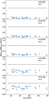 |
Fig. 3 Relative standard deviations of the distance offsets obtained with the LCTs over those obtained with the simple average. The ratios are plotted as a function of dtrue. From top to bottom, the photometric error adopted for the simulation increases. The distances were obtained with PL(i) relations and mean magnitudes from single-point LCT anchoring. |
4.3.1 Distances from PL(i) and PL(z); single point anchoring
We tested the case for distances derived both with the PL(¿) and PL(z), using the single point anchor approach. We found that the σ of the offsets are a factor ~1.5-to-7 smaller when using the LCTs. Figures 3 and 4 show a decreasing trend of the ratio with decreasing photometric error. We also note that the < δd[L/s](n,σ) > are closer to zero when using LCTs with respect to the simple mean. By looking at the absolute values, using the LCTs, σ drops below 1 kpc in all cases, and below ~0.5 kpc when the photometric error is smaller than 0.050 mag. This means relative uncertainties smaller than ~5–10% in the two cases. As expected, when the period, Ampl and reference epoch of the variable are well known, and one can assume that there was no phase shift or significant period change between the observations and the time series adopted to derive the pulsation properties, applying the LCT is always an advantage.
4.3.2 Distances from PL(i) and PL(z); LCT fitting at fixed amplitude
We have checked the behavior of distances obtained from PL(i) and PL(z), using also the mean magnitudes derived with the LCT fitting at fixed Ampl. Figs. A.1 and A.2 display the ratio of the standard deviations of the distance offsets in the two cases of LCT fitting and simple average. The trend with photometric error is the same as for the single-point anchoring case: with increasing photometric error, the LCTs are less convenient with respect to the simple average. Nonetheless, LCTs still provide a better precision in the majority of cases, at least if the number of phase points is larger than four, or the photometric error is smaller than 0.020 mag. We note that, for distances obtained with the PL(z), the LCTs are not as effective as for PL(i). This might be due (1) to the smaller number of LCTs for the z band, meaning that the variability of light curve morphology cannot be as well sampled as for the ɡ, r and i bands; (2) to the fact that we do not have z-band RRc LCTs: RRc are easier to fit due to their almost sinusoidal light curves and not having them might worsen the average ratios of the z band.
4.3.3 Distances from PW(r,g-r); LCT fitting at free amplitude
Fig. A.3 displays the ratios of offsets obtained by estimating the distances with the PW(r,ɡ – r) for halo stars. In this case, the improvement in the standard deviations can be as high as a factor 12, with the most significant improvements obtained when the photometric error is small. There are a few cases in which the precision on the distance estimate is generally worse when using the template, more specifically when only four points are available and the photometric error is larger than 0.010 mag. This is consistent with what we found for < mag > offsets. We therefore advise adopting the LCT fitting with free Ampl when more than four points are available or when the photometric error is 0.01 mag or lower.
5 Summary and final remarks
We have built LCTs of RRLs in the ɡri LSST passbands for both RRab and RRc type stars as well as LCTs in the z LSST passband for RRab. These were conceived to enhance the science performed with early data from the Rubin Observatory, improving the mean magnitude and distance estimate or RRLs, which are valuable Galactic structures and formation probes since they trace the very old population (Layden 1994; Fabrizio et al. 2019; Iorio & Belokurov 2021).
In total, we delivered a set of 37 LCTs in analytical form, providing the coefficients of the Fourier series (up to the 40th order) representing them. The LCTs of RRab highlight, as expected, the known behavior of this pulsation type, with light curves that are increasingly asymmetrical and with steeper rising branches at bluer bands and shorter periods. On the other hand, RRc LCTs display the well-known almost sinusoidal morphology, with either a hump or a flattening before the maximum of pulsation.
We have tested our LCTs using three different methods: (1) the classical LCT anchoring to a single observed phase point (Jones et al. 1996); (2) the LCT fitting, where, if at least three observed phase points are available, one can use the LCT as a fitting function, minimizing the χ2 on two free parameters (phase offset and magnitude offset) (Braga et al. 2019); (3) the LCT fitting with free amplitude, which is the brand new approach proposed in this paper – if at least four observed phase points are available, one can use the LCT as a fitting function, minimizing the χ2 on three free parameters (phase offset, magnitude offset, and the amplitude of the LCT). The latter will be particularly helpful for the main applications of these LCTs, namely, early science of newly discovered RRLs by LSST. In the first one to two years, for hundreds of thousands of previously unknown RRLs, LSST will provide reliable periods, but since these will be new candidates, one will have no information on their pulsation properties, including the amplitude. Therefore, being able to apply LCTs without the need of knowing the amplitude will mean having a sample of RRLs with precise distances of at least a factor of two to three larger on which to base any Galactic archaeology investigation.
We checked that, in almost all cases, the LCTs do provide better mean magnitudes and distances, but there are a few exceptions. More specifically, when either the number of observations is very low, meaning around four, or the LSST photometric uncertainty is large (≳0.05 mag), one should pay attention and consider just calculating the mean magnitudes as simple flux averages. This means that, in the very first months of the survey, when only 3–5 observations per target will be available, we recommend to apply the templates only on objects brighter than r ~23 mag. However, starting with DR1, we recommend to adopt LCTs on all available targets, based on our quantitative validation.
We also report an interesting finding. The LCTs in this work were derived for the LSST photometric system but using data in the ZTF and DECam photometric systems. Thus, an important part of our work was the comparison of the RRL light curves in these three systems, especially concerning the amplitude ratios (see Appendix D). These are crucial for two reasons. First of all, our investigation of the amplitude ratios allowed us to quantitatively validate the usability of our LCTs with the Rubin Observatory data. Secondly, once we certified that the ZTF, DECam, and LSST amplitudes are the same within 1σ, we compared the ɡrizZ amplitudes also with the Gaia G and OGLE (VI) amplitudes to provide amplitude ratios to be used for the conversion of the amplitudes of known RRLs in these large surveys into ɡrizL amplitudes. This work has unveiled some interesting results. On one side, the ratios  display a behavior similar to that of the RRLs of ω Cen (Braga et al. 2018), with RRc stars having a higher ratio than RRab in bluer bands (ɡZrZ) and a similar ratio at redder bands (iZzD). However, we also found an unexpected and completely new behavior concern-ing the ratios
  of RRab. We found that for bulge RRLs, this ratio follows a positive trend with the period, while in the LMC and SMC, the ratio is constant. Both blending and metal-licity might be playing a role, but it is not within the aim of this paper to investigate this feature.
Finally, we mention that we are aware that another group is submitting a similar work (Baeza-Villagra, in prep.). However, our works are completely independent and based on different datasets, and our LCTs have different purposes.
Data availability
Tables 2, 4, 5, A.1, A.2, A.3, A.4, A.5, A.6 are available at the CDS via anonymous ftp to cdsarc.cds.unistra.fr (130.79.128.5) or via https://cdsarc.cds.unistra.fr/viz-bin/cat/J/A+A/689/A349
The code needed to apply the light curve templates is publicly available at https://github.com/vfbraga/RRL_lcvtemplate_griz_LSST
Acknowledgements
Based on observations obtained with the Samuel Oschin 48-inch Telescope at the Palomar Observatory as part of the Zwicky Transient Facility project. ZTF is supported by the National Science Foundation under Grant No. AST-1440341 and a collaboration including Caltech, IPAC, the Weiz-mann Institute for Science, the Oskar Klein Center at Stockholm University, the University of Maryland, the University of Washington, Deutsches Elektronen-Synchrotron and Humboldt University, Los Alamos National Laboratories, the TANGO Consortium of Taiwan, the University of Wisconsin at Milwaukee, and Lawrence Berkeley National Laboratories. Operations are conducted by COO, IPAC, and UW. V.F.B. acknowledges the INAF projects ‘‘Participation in LSST – Large Synoptic Survey Telescope” (LSST inkind contribution ITA-INA-S22, PI: G. Fiorentino), OB.FU. 1.05.03.06 and “MINI-GRANTS (2023) DI RSN2” (PI: G. Fiorentino), OB.FU. 1.05.23.04.02. M.Mo. and V.F.B acknowledge financial support from the ACIISI, Consejería de Economía, Conocimiento y Empleo del Gobierno de Canarias and the European Regional Development Fund (ERDF) under the grant with reference ProID2021010075. M.Mo. acknowledges support from Spanish Ministry of Science, Innovation and Universities (MICIU) through the Spanish State Research Agency under the grants “RR Lyrae stars, a lighthouse to distant galaxies and early galaxy evolution” and the European Regional Development Fun (ERDF) with reference PID2021-127042OB-I00 and from the Severo Ochoa Programe 2020-2023 (CEX2019-000920-S). M.D.O. achknowledges the INAF GO Project: “The GAlactic bulGE with pleiadi” (PI: M. Dall’Ora), OB.FU.: 1.05.23.05.24. M.Ma. acknowledges Project PRIN MUR 2022 (code 2022ARWP9C) “Early Formation and Evolution of Bulge and HalO (EFEBHO)”, PI: Marconi, M., funded by European Union - Next Generation EU and Large grant INAF 2023 MOVIE (PI: M. Marconi). C.G. acknowledges support from AEI-MCINN under grant “At the forefront of Galactic Archaeology: evolution of the luminous and dark matter components of the Milky Way and Local Group dwarf galaxies in the Gaia era” with reference PID2020-118778GB-I00/10.13039/501100011033 and from the Spanish Ministry of Science, Innovation and University (MICIN) through the Spanish State Research Agency, under Severo Ochoa Centres of Excellence Programme 2020-2023 (CEX2019-000920-S). R.S. acknowledges SNN-147362 and the KKP-137523 ‘Seismo-Lab’ Élvonal grants of the Hungarian Research, Development and Innovation Office (NKFIH). This work was also supported by the NKFIH excellence grant TKP2021-NKTA-64.
Appendix A Additional material
Hereby, we display the tables and figures that are too large to be put within the text and would severely affect the readability of the paper.
Pulsation, fitting, and light curve properties of the ZTF ɡri light curves of RRLs.
Coefficients of the LCTs and parameters used to derive them.
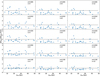 |
Fig. A.1 Same as Fig. 3 but the mean magnitudes were obtained by fitting the simulated time series with the LCT with fixed amplitude. |
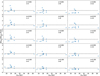 |
Fig. A.2 Same as Fig. 3 but the mean magnitudes were obtained by fitting the simulated time series with the LCT with fixed amplitude and the distances were obtained with PL(z) relations. |
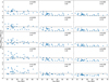 |
Fig. A.3 Same as Fig. 3 but the mean magnitudes were obtained by fitting the simulated time series with the LCT with free amplitude and the distances were obtained with PW(r,𝑔 – r) relations. |
Averages and standard deviations of the δL(n,σ) with fixed amplitudes.
Averages and standard deviations of the δA(n,σ) with fixed amplitudes.
Averages and standard deviations of the δL(n,σ) with free amplitudes.
Averages and standard deviations of the δA(n,σ) with free amplitudes.
Appendix B Figures of the light curve templates
Figs. B.1, B.2 and B.3 make immediately clear that, for the RRc, the LCTs at shortest period are significantly different from other periods. In fact, they display a clear shoulder before the real pulsation maximum while, at longer periods, a flattening of the sinusoid appears. This is, in principle, in agreement with the suggestion of a hump progression with the period of RRc (Petersen 1984). However, we cannot draw firm conclusions from this feature, because: 1) metallicity plays a role and we do not have iron abundance estimates for a sizeable sample of our RRLs; 2) data for long-period RRc are a factor of 30-60 less than data for shorter-period RRc, meaning that a comparison might be misleading.
One can also notice that, in the i band, the two bins with longer periods (0.31-0.39 days and 0.39-0.43 days) display a clear difference that spans almost half of the pulsation cycle. However, in the g and r bands, the LCTs are very similar, with small differences (≲ 0.05 normalized mag) only around the maximum. Nonetheless, we decided to keep the same bin separation in all bands, including g and r, to have a homogeneous binning of the periods for RRc.
Concerning RRab (Figs. B.4, B.5, B.6 and B.7), the change in shape of the LCTs is progressive for all period ranges and passbands. Unfortunately, for the long-period RRLs (0.71-0.83 days), we do not have enough z-band data to clearly reproduce the hump before maximum light. This feature is visible in all other bands, especially 𝑔 and r, where it starts to appear already in the 0.65-0.71 days bin.
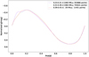 |
Fig. B.1 LCTs of RRc in the passband 𝑔. |
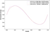 |
Fig. B.2 LCTs of RRc in the passband r. |
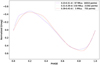 |
Fig. B.3 LCTs of RRc in the passband i. |
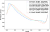 |
Fig. B.4 LCTs of RRab in the passband 𝑔. |
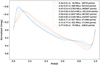 |
Fig. B.5 LCTs of RRab in the passband r. |
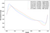 |
Fig. B.6 LCTs of RRab in the passband i. |
 |
Fig. B.7 LCTs of RRab in the passband z. |
Appendix C Comparison with Sesar 2010 templates
Within a study of the spatial distribution of halo RRLs, S10 developed LCTs of RRLs in the SDSS u𝑔riz passbands. Since we demonstrated, in sections 3.6 and D that there are no relevant differences between all the uriz photometric systems, one might think that to develop new LCTs is not necessary. However, by construction, S10 LCTs are not associated to any pulsation property, except the pulsation mode. This approach allowed S10 to deliver a set of LCTs covering all morphologies, and to be as general as possible, but this also means that, anyone wanting to use S10 LCTs for mean magnitude estimates, cannot know which specific LCT to adopt for a given target, since no pulsation property is associated to these LCTs.
A practical example for the g passband, where 22 RRab LCTs are available in S10: even having all the pulsation properties available for a target and being able to correctly anchor the LCTs to any single observed phase point, one would have no way to decide which is the best LCT to use. Even when several phase points are available, one would still have to perform 22 fits instead of one, and only then it would be possible to select the best LCT. This means to increase the computing time by more than one order of magnitude for each target.
Aside from these difficulties in applying S10 LCTs, there are quantitative reasons for having developed our new LCTs. First of all, our database consists on more than 28000 light curves versus ∼2500 for S10). Secondly, our halo sample (ZTF) covers the entire sky above declination –20 degrees, while S10 sample is limited to the Stripe 82 region of the SDSS survey, where substructures may more easily bias the properties of RRLs due to an anomalous metallicity distribution, for example.
Appendix D Amplitude ratios between different photometric systems
In the following, we provide light amplitude ratios between the most commonly used photometric systems. More precisely, we derived the following amplitude ratios:
the LSST uriz over 𝑔 ratios
the LSST over DECam u𝑔rizy ratios
the LSST over ZTF 𝑔r ratios
the LSST over SDSS 𝑔r ratios
the ZTF/DECam over I ratios
the ZTF/DECam over Gaia (G) ratios
the OGLE I over V ratios
For the ratios between amplitudes in the same band but of different photometric systems, we adopt the following notation: r(x)A/B is the ratio of Ampl between the x bands of the A and B photometric systems, for example,  .
.
Since we have no available empirical LSST light curves, the only way to estimate r(𝑔)L/D, r(𝑔)L/z and the LSST  ratios was to adopt synthetic light curves obtained from stellar pulsation models (Marconi et al. 2015, 2022). For this purpose, we adopted models at Z=0.0003, Z=0.001 and Z=0.008, which are typical abundances for RRLs for the metal-poor end, the peak of the Galactic halo and the metal-rich tail, respectively (Fabrizio et al. 2021; Mullen et al. 2022; Cabrera Garcia et al. 2024).
Unfortunately, synthetic light curves are only available in the LSST and DECam passbands, but not in the ZTF. Therefore, we first derived r(x)L/D directly from pulsation models and then we obtained the r(x)L/z ratios by multiplying r(x)L/D by r(x)Z/D. The latter ratios (r(x)z/D) were obtained from observed light curves of objects in common between DECam and ZTF, namely, RRLs in the globular cluster M5. We note that the photometric reduction process of the M5 data in Vivas et al. (2017) is the same as that adopted for bulge data by Saha et al. (2019).
D.1 LSST uriɀ over 𝑔 ratios
Figure D.1 displays, in the left and right panels respectively, the ratios  versus periods of the RRc and RRab stars, color-coded by metallicity. The mean and standard deviations of the ratios are reported in Table D.1 and displayed as solid and dashed lines in the figure, respectively. Four facts are immediately clear: 1) the ratios at fixed metallicity span a very narrow range; 2) almost all the mean ratios of RRab and RRc stars match within 1σ; 3) the ratio
  of RRab stars seems to follow a V shape; 4) The
  of both RRab and RRc displays a positive trend with metallicity. The LSST will be the only photometric survey that allows one to empirically check these ratios, thanks to its unprecedented multiband coverage.
D.2 LSST over DECam ugriɀy ratios
Figure D.2 displays, in the a)-f) and g)-l) right panels, the ratios r(x)L/D versus periods of the RRc and RRab stars, respectively. First of all we note that, within the dispersion, the ratios can be assumed to be constant with period. The only, marginal exceptions are r(u)L/D (that is useless for our templates) which displays a V-shape and r(ɀ)L/D band for RRab. We note, however, that the range of variation of these ratios is, at most 0.05. This corresponds to a 1-5% error on the estimate of Ampl, which is significantly less than typical errors on Ampl (Braga et al. 2022). Table D.1 displays the average ratios and the standard deviations. To sum up, the r(x)L/D ratios are close to 1, with a maximum offset of ~0.06 (if we exclude the u band which is not useful for our templates). The standard deviations are also very small, being at most 0.01.
D.3 LSST over ZTF 𝑔r ratios
As already mentioned, we have no way to directly compare LSST and ZTF data, neither empirically nor synthetically. Therefore, we had to follow a two-step process, first deriving r(x)Z/D and then obtaining  . The r(x)Z/D ratios were obtained from empirical data and are displayed in Fig. D.3. It is immediately clear that both r(𝑔)Z/D and r(r)Z/D are consistent, within the dispersion, with a ratio of 1, meaning that also r(x)L/Z is 1, within the errors. The values are listed in Table D.1. Unfortunately, we do not have any data in common for the i band, meaning that we cannot quantitatively derive r(i)Z/D. The fact that both r(x)L/D and r(x)L/Z are consistent with one, well within one sigma, means that even though our LCTs were built based on ZTF and DECam data, they can be used on LSST data, which is our main aim.
D.4 LSST over SDSS 𝑔r ratios
The survey SDSS (Almeida et al. 2023) is one of the most extensive photometric surveys, and it is the one that popularized the u𝑔riɀ(y) photometric system. Therefore, we also derived amplitude ratios between the LSST and the SDSS photometric system (r(x)L/S). These ratios will be useful when applying the LCTs to RRLs with known amplitudes from SDSS. Also in this case, we must follow a two-step process: 1) We derive r(x)Z/S ratios, and 2) we obtain r(x)L/S = r(x)L/Z · r(x)Z/S. The reference photometric system that we used is ZTF because it is the dataset for which we could find more matches with the RRLs found by Sesar et al. (2010) in the Stripe 82 of SDSS. The results are displayed in Fig. D.4 and Fig. D.6, and listed in Table D.1. The r(x)Z/S ratios are all consistent with 1 within the standard deviations, with the only, marginal exception of r(r)Z/S of the RRc. Finally, we derived also the r(x)L/S ratios by multiplying r(x)L/Z by r(x)Z/S. The behavior of r(r)L/S is identical to that of r(x)Z/S: all the values are 1 within the standard deviations, again with the only exception of r(r)L/S (see Table D.1).
D.5 ZTF/DECam over I ratios
An ongoing extensive optical survey specifically conceived for micro-lensing and variability detections (Udalski et al. 1992, 2015), OGLE provides an outstanding combination of time, sky, and depth coverage on top of time series with 103–104 measurements per star in the Johnson-Cousins V and I band. It also has a far better pixel scale than ASAS-SN (0.25 vs 8.0 arcseconds). Since, to this point in the paper, we still miss an anchor to the Johnson system, we calculated the ZTF over OGLE ratios. In Fig. D.6, we note that the  and
and  ratios display a clear separation between ab and c type RRLs, the latter having higher ratios. On the other hand, the
  ratios of RRab and RRc are similar. Differences in amplitude ratio between RRc and RRab were found by Braga et al. (2018) in ω Cen. More specifically, they found that the NIR-to-V-band amplitude ratios of RRab are larger than RRc. This is consistent with our result because the difference between the RRc and RRab ratios progressively decreases from 𝑔Z to rZ to iZ, where the difference is zero. Unfortunately, the overlap between our DECam sample and OGLE for the iD and ɀD bands is small, and the dispersion is very large. Thus, it does not allow us to draw firm quantitative conclusions.
We also derived the ratios between Ampl(ɀD) and Ampl(I), by matching the estimates of Ampl(I) from Neeley (2017) and Ampl(ɀD) by Vivas et al. (2017). Although the sample is very small and shows a large dispersion, it follows the quoted trend. Finally, we derived  for bulge RRab matched with OGLE (blue points in Fig. D.6). We found an average and standard deviation of 0.947±0.085, which is almost identical to the one obtained with M5 data. This is encouraging but also expected, because M5 I-band photometry is calibrated to the Kron-Cousins system, as OGLE. However, for homogeneity, in Table D.1, we provide only the ratios from M5 data, since these can be estimated for both RRab and RRc.
D.6 ZTF/DECam over Gaia (G) ratios
The photometric system of Gaia (G, Bp, Rp) has become of primary importance for variable stars, since Gaia delivered catalogs and photometric properties for millions of variable stars, among which, the largest homogeneous catalog of known RRLs (Clementini et al. 2023). Moreover, LSST brokers in a manner similar to Alerce (Sánchez-Sáez et al. 2021), and ANTARES (Matheson et al. 2021) will provide cross-identification of LSST candidate variables with Gaia. Therefore, it is crucial to also provide amplitude ratios versus Ampl(G)—as obtained from the peak_to_peak_𝑔 column in the gaiadr3. vari_rrlyrae table within Gaia DR3, which will allow LCT users to adopt Gaia as a starting catalog. As described in Sect. 2.1, we already have Gaia -ZTF matching. By selecting only RRLs with photometric properties in Gaia DR3, we ended up with 23610 RRLs. The RRab and RRc display the same ratio in the 𝑔Z and rZ bands. In the iZ and ɀD bands, the ratio of the RRab is higher than that of RRc (but still within 1σ), following the same trend displayed by the ratios over Ampl(I) displayed in Fig. D.6. We point out that, for the ɀD ratios, we used a match between Gaia DR3 and M5 photometry from Vivas et al. (2017), although the overlap of DECam bulge sample with Gaia DR3 is larger. This is because bulge RRLs are very faint in Gaia (G >18) and could be either affected by blending or by second-order extinction effects. In fact, we found that  for bulge RRLs is significantly higher (0.763+0.110) than that of M5 (0.679+0.076). We propose three possible explanations: 1) an underestimated Ampl(G) in bulge RRLs, as expected from blended sources; 2) an underestimated Ampl(G) in bulge RRLs due to foreground reddening. The latter hypothesis was tested, under suggestion of the referee, by checking the trend of Ampl(G) with the Bp – Rp color, revealing a decreasing trend for the high-amplitude RRLs. We ruled out the hypothesis that this difference is due to an insufficient number of G-band observations in the bulge, since neither Ampl(G) nor
  seem to depend on that.
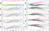 |
Fig. D.1 Amplitude ratios in the LSST passbands for RRab from pulsation models. Left panels (a-e), from top to bottom: |

D.7 OGLE I over V ratios
Finally, we provide the amplitude ratios between the Johnson-Kron-Cousins V and I bands using OGLE data, in order to dispose of ratios allowing us to convert Ampl from the historical standard Johnson V to the LSST photometric systems. Unfortunately, the OGLE consortium does not provide Ampl(V), so we fitted the V-band light curves available and calculated the amplitudes. For this task, we adopted the same Fourier series fitting method with an automatic selection of the degree that we used for the ZTF data. To keep only the best estimates, we rejected all the light curves whose average errors were too large (>0.15 mag), those with less than 30 phase points, and those with gaps in phase larger than 0.08 to avoid nonrealistic ripples and bumps in the Fourier series fits.
We found a very notable and completely new behavior different behavior between the LMC/SMC and bulge (BUL) sample of OGLE RRLs. In fact, while the LMC and SMC ratios display a flat behavior, the BUL sample clearly show that the ratios are strictly increasing with period, both for RRc and RRab. By leaving the slope free to change in the LMC sample, the maximum slope is around one quarter than that of the BUL sample. The SMC sample is too small to allow for a similar, quantitatively meaningful investigation. Since the analysis of the data was performed homogeneously on the different datasets, we have to assume that this trend is an intrinsic feature of BUL RRLs. It is not the aim of this paper to delve deep into this feature, but we advance two preliminary hypotheses. The first is that the trend in the bulge is due to blending. However, preliminary considerations tell us that, in the bulge, redder wavelengths (I) should be more affected than blue wavelengths (V). This means that one should observe a decreasing trend because longer-period RRLs generally have redder colors instead of an increasing one. The other possibility is that the higher metallicity of bulge RRLs (Walker 1991) might be playing a role, but to validate this hypothesis, we would need to conduct an extensive investigation with both globular cluster data and pulsation models, which deserves it own paper.
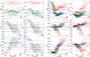 |
Fig. D.2 Amplitude ratios in the LSST passbands for RRc from pulsation models. Left panels (a-f), from top to bottom, left to right: r(x)L/D amplitude ratios versus pulsation period for Z=0.0003 (blue), Z=0.001 (green), Z=0.008 (red) RRc models. Solid/dashed lines display the average/standard deviations of each set of models. Right panels (g-l): Same as left but for the RRab models. |
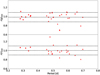 |
Fig. D.3 ZTF versus DECam passband amplitude ratios. Left: r(𝑔)Z/D (top) and r(r)Z/D (bottom) versus Ampl(𝑔)Z and Ampl(r)Z, respectively, of the RRLs for which we have light curves from both DECam and ZTF. Right: Same as left but for ZTF vs SDSS photometric systems. |
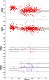 |
Fig. D.5 Amplitude ratios between (from top to bottom) Ampl(𝑔Z), Ampl(rZ), Ampl(iZ), and Ampl(ɀD) over Ampl(I). Blue points in the bottom panel represent the amplitude ratios derived from bulge RRLs. |
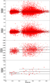 |
Fig. D.6 Amplitude ratios between (from top to bottom) Ampl(𝑔Z), Ampl(rZ), Ampl(iZ), and Ampl(ɀD) over Ampl(G). |
Amplitude ratios between the LSST (suffix L), DECam (suffix D), ZTF (suffix Z), Gaia (G) and OGLE Johnson-Kron-Cousins (VI).
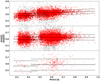 |
Fig. D.7 OGLE passbands amplitude ratios. Top: |

References
- Almeida, A., Anderson, S. F., Argudo-Fe?nández, M., et al. 2023, ApJS, 267, 44 [NASA ADS] [CrossRef] [Google Scholar]
- Bailey, S. I. 1902, Ann. Harvard Coll. Observ., 38 [Google Scholar]
- Bellm, E. C., Kulkarni, S. R., Graham, M. J., et al. 2019, PASP, 131, 018002 [Google Scholar]
- Bianco, F. B., Ivezic, Ž., Jones, R. L., et al. 2022, ApJS, 258, 1 [NASA ADS] [CrossRef] [Google Scholar]
- Bobrick, A., Iorio, G., Belokurov, V., et al. 2024, MNRAS, 527, 12196 [Google Scholar]
- Bono, G., Caputo, F., Castellani, V., et al. 2003, MNRAS, 344, 1097 [Google Scholar]
- Braga, V. F., Dall’Ora, M., Bono, G., et al. 2015, ApJ, 799, 165 [NASA ADS] [CrossRef] [Google Scholar]
- Braga, V. F., Stetson, P. B., Bono, G., et al. 2016, AJ, 152, 170 [Google Scholar]
- Braga, V. F., Stetson, P. B., Bono, G., et al. 2018, AJ, 155, 137 [NASA ADS] [CrossRef] [Google Scholar]
- Braga, V. F., Stetson, P. B., Bono, G., et al. 2019, A&A, 625, A1 [NASA ADS] [CrossRef] [EDP Sciences] [Google Scholar]
- Braga, V. F., Crestani, J., Fabrizio, M., et al. 2021, ApJ, 919, 85 [NASA ADS] [CrossRef] [Google Scholar]
- Braga, V. F., Fiorentino, G., Bono, G., et al. 2022, MNRAS, 517, 5368 [NASA ADS] [CrossRef] [Google Scholar]
- Cabrera Garcia, J., Beers, T. C., Huang, Y., et al. 2024, MNRAS, 527, 8973 [Google Scholar]
- Cacciari, C., Corwin, T. M., & Carney, B. W. 2005, AJ, 129, 267 [NASA ADS] [CrossRef] [Google Scholar]
- Catelan, M., Pritzl, B. J., & Smith, H. A. 2004, ApJS, 154, 633 [Google Scholar]
- Clementini, G., Ripepi, V., Garofalo, A., et al. 2023, A&A, 674, A18 [NASA ADS] [CrossRef] [EDP Sciences] [Google Scholar]
- DePoy, D. L., Abbott, T., Annis, J., et al. 2008, SPIE Conf. Ser., 7014, 70140E [NASA ADS] [Google Scholar]
- Di Criscienzo, M., Leccia, S., Braga, V., et al. 2023, ApJS, 265, 41 [NASA ADS] [CrossRef] [Google Scholar]
- Fabrizio, M., Bono, G., Braga, V. F., et al. 2019, ApJ, 882, 169 [Google Scholar]
- Fabrizio, M., Braga, V. F., Crestani, J., et al. 2021, ApJ, 919, 118 [NASA ADS] [CrossRef] [Google Scholar]
- Fiorentino, G., Bono, G., Monelli, M., et al. 2015, ApJ, 798, L12 [Google Scholar]
- Gaia Collaboration (Prusti, T., et al.) 2016, A&A, 595, A1 [NASA ADS] [CrossRef] [EDP Sciences] [Google Scholar]
- Inno, L., Matsunaga, N., Romaniello, M., et al. 2015, A&A, 576, A30 [NASA ADS] [CrossRef] [EDP Sciences] [Google Scholar]
- Iorio, G., & Belokurov, V. 2021, MNRAS, 502, 5686 [Google Scholar]
- Jones, R. V., Carney, B. W., & Fulbright, J. P. 1996, PASP, 108, 877 [NASA ADS] [CrossRef] [Google Scholar]
- Jurcsik, J., & Kovacs, G. 1996, A&A, 312, 111 [Google Scholar]
- Jurcsik, J., & Juhász, Á. 2022, MNRAS, 517, 1907 [NASA ADS] [CrossRef] [Google Scholar]
- Kiss, L. L., Csák, B., Thomson, J. R., & Vinkó, J. 1999, A&A, 345, 149 [NASA ADS] [Google Scholar]
- Kovacs, G., & Jurcsik, J. 2023, A&A, 678, A138 [NASA ADS] [CrossRef] [EDP Sciences] [Google Scholar]
- Kunder, A., Stetson, P. B., Cassisi, S., et al. 2013, AJ, 146, 119 [CrossRef] [Google Scholar]
- Layden, A. C. 1994, AJ, 108, 1016 [Google Scholar]
- Leavitt, H. S. 1908, Ann. Harvard Coll. Observ., 60, 87 [NASA ADS] [Google Scholar]
- Longmore, A. J., Fernley, J. A., & Jameson, R. F. 1986, MNRAS, 220, 279 [NASA ADS] [Google Scholar]
- LSST Science Collaboration (Abell, P. A., et al.) 2009, arXiv e-prints [arXiv:0912.0201] [Google Scholar]
- Madore, B. F. 1982, ApJ, 253, 575 [NASA ADS] [CrossRef] [Google Scholar]
- Madore, B. F., & Freedman, W. L. 1991, PASP, 103, 933 [Google Scholar]
- Madore, B. F., Hoffman, D., Freedman, W. L., et al. 2013, ApJ, 776, 135 [Google Scholar]
- Marconi, M., Coppola, G., Bono, G., et al. 2015, ApJ, 808, 50 [Google Scholar]
- Marconi, M., Molinaro, R., Dall’Ora, M., et al. 2022, ApJ, 934, 29 [NASA ADS] [CrossRef] [Google Scholar]
- Martínez-Vázquez, C. E., Monelli, M., Gallart, C., et al. 2016, MNRAS, 461, L41 [Google Scholar]
- Masci, F. J., Laher, R. R., Rusholme, B., et al. 2019, PASP, 131, 018003 [Google Scholar]
- Matheson, T., Stubens, C., Wolf, N., et al. 2021, AJ, 161, 107 [NASA ADS] [CrossRef] [Google Scholar]
- Matsunaga, N., Itane, A., Hattori, K., et al. 2022, ApJ, 925, 10 [CrossRef] [Google Scholar]
- Mullen, J. P., Marengo, M., Martínez-Vázquez, C. E., et al. 2022, ApJ, 931, 131 [NASA ADS] [CrossRef] [Google Scholar]
- Narloch, W., Hajdu, G., Pietrzynski, G., et al. 2024, A&A, 689, A138 [NASA ADS] [CrossRef] [EDP Sciences] [Google Scholar]
- Neeley, J. R. 2017, PhD thesis, Iowa State University, USA [Google Scholar]
- Ngeow, C.-C., Bhardwaj, A., Dekany, R., et al. 2022, AJ, 163, 239 [NASA ADS] [CrossRef] [Google Scholar]
- Oosterhoff, P. T. 1939, The Observatory, 62, 104 [NASA ADS] [Google Scholar]
- Petersen, J. O. 1984, A&A, 139, 496 [NASA ADS] [Google Scholar]
- Prudil, Z., Dékány, I., Grebel, E. K., & Kunder, A. 2020, MNRAS, 492, 3408 [Google Scholar]
- Rodríguez, E., Arellano Ferro, A., Costa, V., López-González, M. J., & Sareyan, J. P. 2003, A&A, 407, 1059 [NASA ADS] [CrossRef] [EDP Sciences] [Google Scholar]
- Saha, A., Vivas, A. K., Olszewski, E. W., et al. 2019, ApJ, 874, 30 [NASA ADS] [CrossRef] [Google Scholar]
- Sánchez-Sáez, P., Reyes, I., Valenzuela, C., et al. 2021, AJ, 161, 141 [CrossRef] [Google Scholar]
- Schwarzschild, M. 1940, Harvard Coll. Observ. Circ., 437, 1 [Google Scholar]
- Sesar, B., Ivezic, Ž., Grammer, S. H., et al. 2010, ApJ, 708, 717 [NASA ADS] [CrossRef] [Google Scholar]
- Skowron, D. M., Skowron, J., Mróz, P., et al. 2019, Acta Astron., 69, 305 [NASA ADS] [Google Scholar]
- Soszynski, I., Udalski, A., Wrona, M., et al. 2019, Acta Astron., 69, 321 [NASA ADS] [Google Scholar]
- Stothers, R. B. 1987, ApJ, 319, 260 [NASA ADS] [CrossRef] [Google Scholar]
- Udalski, A., Szymanski, M., Kaluzny, J., Kubiak, M., & Mateo, M. 1992, Acta Astron., 42, 253 [NASA ADS] [Google Scholar]
- Udalski, A., Szymanski, M. K., & Szymanski, G. 2015, Acta Astron., 65, 1 [Google Scholar]
- van Albada, T. S., & Baker, N. 1971, ApJ, 169, 311 [NASA ADS] [CrossRef] [Google Scholar]
- VanderPlas, J. T., & Ivezic, Ž. 2015, ApJ, 812, 18 [NASA ADS] [CrossRef] [Google Scholar]
- Vivas, A. K., Saha, A., Olsen, K., et al. 2017, AJ, 154, 85 [NASA ADS] [CrossRef] [Google Scholar]
- Walker, A. R. 1991, in IAU Symposium, 148, The Magellanic Clouds, eds. R. Haynes, & D. Milne, 307 [Google Scholar]
- Walker, A. R., & Terndrup, D. M. 1991, ApJ, 378, 119 [NASA ADS] [CrossRef] [Google Scholar]
Modified version of UniformityMetric by Peter Yoachim (https://rubin-sim.lsst.io/api/rubin_sim.maf. metrics.UniformityMetric.html#rubin_sim.maf.metrics. UniformityMetric), to compute how uniformly the observations are spaced in phase
These correspond to the expected photometric error on the single visit for a star of magnitude r ~20.2, 21.0, 22.0, 23.2 and 24.0 within the LSST (LSST Science Collaboration 2009).
All Tables
Pulsation, fitting, and light curve properties of the ZTF ɡri light curves of RRLs.
Amplitude ratios between the LSST (suffix L), DECam (suffix D), ZTF (suffix Z), Gaia (G) and OGLE Johnson-Kron-Cousins (VI).
All Figures
|
Fig. 1 Period distributions and Bailey diagrams of our ZTF and DECAM RRLs. Left panels, from top to bottom: period distribution of the RRLs adopted to build the templates in the 𝑔ZrZiZzD bands. The RRab are displayed in red and RRc in blue. The red and blue dashed lines display the period thresholds of the LCTs derived in this work, for RRab and RRc, respectively. Right panels: same as left but for the Bailey diagram (period versus Ampl). Dashed black lines display the loci of the Oosterhoff tracks derived by Fabrizio et al. (2019) and transformed into the 𝑔ZrZiZzD bands using the ratios derived in Appendix D. |
| In the text | |
|
Fig. 2 Density plot of a CNLCV (𝑔 band, RRab, period bin [0.35–0.41 days]). Darker cells are the most dense. The red crosses display the average of the four highest-density cells at each phase. The green, solid line shows the Fourier fit of these average points. |
| In the text | |
|
Fig. 3 Relative standard deviations of the distance offsets obtained with the LCTs over those obtained with the simple average. The ratios are plotted as a function of dtrue. From top to bottom, the photometric error adopted for the simulation increases. The distances were obtained with PL(i) relations and mean magnitudes from single-point LCT anchoring. |
| In the text | |
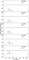 |
Fig. 4 Same as Figure 3 but the distances were obtained with PL(z) relations. |
| In the text | |
|
Fig. A.1 Same as Fig. 3 but the mean magnitudes were obtained by fitting the simulated time series with the LCT with fixed amplitude. |
| In the text | |
|
Fig. A.2 Same as Fig. 3 but the mean magnitudes were obtained by fitting the simulated time series with the LCT with fixed amplitude and the distances were obtained with PL(z) relations. |
| In the text | |
|
Fig. A.3 Same as Fig. 3 but the mean magnitudes were obtained by fitting the simulated time series with the LCT with free amplitude and the distances were obtained with PW(r,𝑔 – r) relations. |
| In the text | |
|
Fig. B.1 LCTs of RRc in the passband 𝑔. |
| In the text | |
|
Fig. B.2 LCTs of RRc in the passband r. |
| In the text | |
|
Fig. B.3 LCTs of RRc in the passband i. |
| In the text | |
|
Fig. B.4 LCTs of RRab in the passband 𝑔. |
| In the text | |
|
Fig. B.5 LCTs of RRab in the passband r. |
| In the text | |
|
Fig. B.6 LCTs of RRab in the passband i. |
| In the text | |
|
Fig. B.7 LCTs of RRab in the passband z. |
| In the text | |
|
Fig. D.1 Amplitude ratios in the LSST passbands for RRab from pulsation models. Left panels (a-e), from top to bottom: |
| In the text | |
|
Fig. D.2 Amplitude ratios in the LSST passbands for RRc from pulsation models. Left panels (a-f), from top to bottom, left to right: r(x)L/D amplitude ratios versus pulsation period for Z=0.0003 (blue), Z=0.001 (green), Z=0.008 (red) RRc models. Solid/dashed lines display the average/standard deviations of each set of models. Right panels (g-l): Same as left but for the RRab models. |
| In the text | |
|
Fig. D.3 ZTF versus DECam passband amplitude ratios. Left: r(𝑔)Z/D (top) and r(r)Z/D (bottom) versus Ampl(𝑔)Z and Ampl(r)Z, respectively, of the RRLs for which we have light curves from both DECam and ZTF. Right: Same as left but for ZTF vs SDSS photometric systems. |
| In the text | |
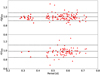 |
Fig. D.4 Same as Fig. D.3 but for the ZTF over SDSS ratios. |
| In the text | |
|
Fig. D.5 Amplitude ratios between (from top to bottom) Ampl(𝑔Z), Ampl(rZ), Ampl(iZ), and Ampl(ɀD) over Ampl(I). Blue points in the bottom panel represent the amplitude ratios derived from bulge RRLs. |
| In the text | |
|
Fig. D.6 Amplitude ratios between (from top to bottom) Ampl(𝑔Z), Ampl(rZ), Ampl(iZ), and Ampl(ɀD) over Ampl(G). |
| In the text | |
|
Fig. D.7 OGLE passbands amplitude ratios. Top: |
| In the text | |
Current usage metrics show cumulative count of Article Views (full-text article views including HTML views, PDF and ePub downloads, according to the available data) and Abstracts Views on Vision4Press platform.
Data correspond to usage on the plateform after 2015. The current usage metrics is available 48-96 hours after online publication and is updated daily on week days.
Initial download of the metrics may take a while.