| Issue |
A&A
Volume 689, September 2024
|
|
|---|---|---|
| Article Number | A207 | |
| Number of page(s) | 8 | |
| Section | Cosmology (including clusters of galaxies) | |
| DOI | https://doi.org/10.1051/0004-6361/202450818 | |
| Published online | 13 September 2024 | |
Re-evaluating the cosmological redshift: Insights into inhomogeneities and irreversible processes
1
Université Paris-Saclay, UVSQ, CNRS, CEA, Maison de la Simulation,
91191
Gif-sur-Yvette,
France
2
Université Paris-Saclay, Université Paris Cité, CEA, CNRS, AIM,
91191
Gif-sur-Yvette,
France
3
Ecole Normale Supérieure de Lyon, CRAL,
UMR CNRS 5574,
69364
Lyon Cedex 07,
France
4
Astrophysics Group, University of Exeter,
Exeter
EX4 4QL,
UK
Received:
21
May
2024
Accepted:
14
July
2024
Abstract
Aims. Understanding the expansion of the Universe remains a profound challenge in fundamental physics. The complexity of solving general relativity equations in the presence of intricate, inhomogeneous flows has compelled cosmological models to rely on perturbation theory in a homogeneous Friedmann–Lemaître–Robertson-Walker background. This approach accounts for a redshift of light encompassing contributions from both the cosmological background expansion along the photon’s trajectory and Doppler effects at emission due to peculiar motions. However, this computation of the redshift is not covariant, as it hinges on specific coordinate choices that may distort physical interpretations of the relativity of motion.
Methods. In this study we show that peculiar motions, when tracing the dynamics along time-like geodesics, must contribute to the redshift of light through a local volume expansion factor, in addition to the background expansion. By employing a covariant approach to redshift calculation, we address the central question of whether the cosmological principle alone guarantees that the averaged local volume expansion factor matches the background expansion.
Results. We establish that this holds true only in scenarios characterised by a reversible evolution of the Universe, where inhomogeneous expansion and compression modes compensate for one another. In the presence of irreversible processes, such as the dissipation of large-scale compression modes through matter virialisation and associated entropy production, the averaged expansion factor becomes dominated by expansion in voids that can no longer be compensated for by compression in virialised structures. Furthermore, for a universe in which a substantial portion of its mass has undergone virialisation, adhering to the background evolution on average leads to significant violations of the second law of thermodynamics. Our approach shows that entropy production due to irreversible processes during the formation of structures plays the same role as an effective, time-dependent cosmological constant (i.e. dynamical dark energy) without the need to invoke new unknown physics. Our findings underscore the imperative need to re-evaluate the influence of inhomogeneities and irreversible processes on cosmological models, shedding new light on the intricate dynamics of our Universe.
Key words: cosmology: theory / large-scale structure of Universe
Corresponding author; This email address is being protected from spambots. You need JavaScript enabled to view it. ; This email address is being protected from spambots. You need JavaScript enabled to view it.
© The Authors 2024
 Open Access article, published by EDP Sciences, under the terms of the Creative Commons Attribution License (https://creativecommons.org/licenses/by/4.0), which permits unrestricted use, distribution, and reproduction in any medium, provided the original work is properly cited.
This article is published in open access under the Subscribe to Open model. This email address is being protected from spambots. You need JavaScript enabled to view it. to support open access publication.
1 Introduction
The comprehension of the recessional velocity of extragalactic objects hinges upon the redshift-distance relation derived from homogeneous solutions of Einstein’s field equations within the framework of the Friedmann–Lemaître–Robertson-Walker (FLRW) metric. Within this coordinate system, the spatial coordinates are comoving with the matter that fills the Universe, attributing the cosmological redshift to the expansion of ‘space’ along the path of photons. However, observations in the nearby Universe have revealed a notable scatter around the linear redshift-distance relation, primarily driven by the presence of peculiar velocities of sources inducing a Doppler shift upon photon emission (Peebles 1993; Peacock 1998). The debate in the literature regarding whether cosmological and Doppler shifts are equivalent phenomena is ongoing (Bunn & Hogg 2009; see also Peacock 1998, 2008; Whiting 2004; Chodorowski 2007). As noted in Bunn & Hogg (2009), the interpretation of space expansion is not entirely satisfactory from a relativistic standpoint, as it relies on a specific choice of coordinates and thus lacks covariance. Conversely, Räsänen (2009) introduced a covariant approach to redshift calculations for an inhomogeneous dust universe. While this approach represents a significant advancement in our understanding of the nature of redshifts in a manner consistent with the covariant framework of general relativity, it has been relatively overlooked. This is largely because, on average, the results do not seem to deviate from the background FLRW expansion in a statistically homogeneous and isotropic universe (Räsänen 2009; Rasanen 2010).
This paper aims to re-evaluate the cosmological redshift by addressing the influence of inhomogeneities and irreversible processes. In Sec. 2, we begin by providing a detailed analysis of the standard interpretation of the redshift within the FLRW metric and discuss the limitations of this approach by using non-comoving coordinates. In the subsequent section (Sec. 3), building on Räsänen (2009), we introduce a covariant approach to the redshift calculation, emphasising the role of peculiar motions and local volume expansion factors. We propose a new approach to the redshift calculation by introducing a tracer of time-like geodesics: the cosmological redshift is associated with the local expansion rate along these time-like geodesics, while the Doppler shifts are associated with the potential non-geodesic motions of the source and observer. Following this, in Sec. 4 we present our findings on the impact of irreversible processes on the cosmological redshift. We argue that in scenarios characterised by irreversible evolution, such as the dissipation of large-scale compression modes through matter virialisation and associated entropy production, the averaged expansion factor is dominated by expansion in voids. This leads to significant violations of the second law of thermodynamics if the Universe’s evolution adheres to the background evolution on average. Lastly, in Sec. 5 we discuss the broader implications of our findings for cosmological models and observations. We conclude in Sec. 6 on the necessity of re-evaluating the influence of inhomogeneities and irreversible processes to better understand the complex dynamics of the Universe.
2 Redshift in a homogeneous expanding universe in non-comoving coordinates
We began with a standard flat FLRW metric with a scale factor, a(t), such that
![Mathematical equation: $\[d s^2=-c^2 d t^2+a^2\left(d r^2+r^2 d \Omega^2\right).\]$](/articles/aa/full_html/2024/09/aa50818-24/aa50818-24-eq1.png) (1)
(1)
The proper distance, R, is
![Mathematical equation: $\[R=a(t) r,\]$](/articles/aa/full_html/2024/09/aa50818-24/aa50818-24-eq2.png) (2)
(2)
and the total velocity is then
![Mathematical equation: $\[\frac{d R}{d t}=H(t) R+a(t) \frac{d r}{d t},\]$](/articles/aa/full_html/2024/09/aa50818-24/aa50818-24-eq3.png) (3)
(3)
with ![Mathematical equation: $\[H \equiv \dot{a} / a\]$](/articles/aa/full_html/2024/09/aa50818-24/aa50818-24-eq4.png) . Within the total velocity, one can discern a contribution originating from the recession velocity due to the expansion of space, and another contribution arising from peculiar velocities vp = a(t)dr/dt. In the late evolution of the Universe, peculiar motions are non-relativistic in the weak field limit. Perturbation theory then leads to the following formulation of the redshift with a cosmological contribution from space expansion and a contribution from the Doppler shift associated with peculiar motions:
. Within the total velocity, one can discern a contribution originating from the recession velocity due to the expansion of space, and another contribution arising from peculiar velocities vp = a(t)dr/dt. In the late evolution of the Universe, peculiar motions are non-relativistic in the weak field limit. Perturbation theory then leads to the following formulation of the redshift with a cosmological contribution from space expansion and a contribution from the Doppler shift associated with peculiar motions:
![Mathematical equation: $\[1+z \approx \exp \left(\int_{t_{\text {src }}}^{t_{\mathrm{dst}}} H d t\right)\left(1+\frac{v_p}{c}\right),\]$](/articles/aa/full_html/2024/09/aa50818-24/aa50818-24-eq5.png) (4)
(4)
assuming for simplicity that the observer at time tdst has no peculiar motion, and the source at time tsrc a peculiar motion vp at emission. With this approach, the inhomogeneities have no significant impact on the redshift, provided that the peculiar velocities remain small vp ≪ c.
We next assumed a perfectly homogeneous FLRW universe with no peculiar motion vp = 0. We wished to apply a local coordinate transformation in a non-comoving frame, characterised by an expansion factor as(t) different from a(t) such that
![Mathematical equation: $\[\begin{aligned}r_d & =r a_d(t) \\t_d & =t+\alpha(r, t),\end{aligned}\]$](/articles/aa/full_html/2024/09/aa50818-24/aa50818-24-eq6.png) (5)
(5)
with as = a/ad and α(r, t) a function that will be specified later, such that td ≈ t at the leading order in ![Mathematical equation: $\[O\left(\dot{a}_d r / c\right)\]$](/articles/aa/full_html/2024/09/aa50818-24/aa50818-24-eq7.png) . We used such a coordinate transformation, locally, such that
. We used such a coordinate transformation, locally, such that ![Mathematical equation: $\[\dot{a}_d r / c\]$](/articles/aa/full_html/2024/09/aa50818-24/aa50818-24-eq8.png) is indeed much smaller than unity. With this transformation, the proper distance R is
is indeed much smaller than unity. With this transformation, the proper distance R is
![Mathematical equation: $\[R=a(t) r=a_s(t) r_d,\]$](/articles/aa/full_html/2024/09/aa50818-24/aa50818-24-eq9.png) (6)
(6)
with as = a/ad. The total velocity is then
![Mathematical equation: $\[\frac{d R}{d t}=H_s(t) R+a_s(t) \frac{d r_d}{d t_d},\]$](/articles/aa/full_html/2024/09/aa50818-24/aa50818-24-eq10.png) (7)
(7)
with ![Mathematical equation: $\[H \equiv \dot{a} / a\]$](/articles/aa/full_html/2024/09/aa50818-24/aa50818-24-eq11.png) . Within the total velocity, one can discern now a contribution originating from the recession velocity due to the expansion of ‘space’, characterised by the scale factor as, and another contribution arising from non-comoving velocities vp,r = asHdrd.
. Within the total velocity, one can discern now a contribution originating from the recession velocity due to the expansion of ‘space’, characterised by the scale factor as, and another contribution arising from non-comoving velocities vp,r = asHdrd.
We chose the function α(r, t) such that the metric in (rd, td) coordinates has only perturbative deviations from a homogeneous metric with a scale factor as. The coordinate transformation verifies
![Mathematical equation: $\[\begin{aligned}d r_d & =a_d d r+r \dot{a}_d d t \\d t_d & =(1+\dot{\alpha}) d t+\alpha^{\prime} d r,\end{aligned}\]$](/articles/aa/full_html/2024/09/aa50818-24/aa50818-24-eq12.png) (8)
(8)
with ![Mathematical equation: $\[\dot{\alpha}\]$](/articles/aa/full_html/2024/09/aa50818-24/aa50818-24-eq13.png) the derivative with respect to t and α′ the derivative with respect to r. This system can be inverted to give
the derivative with respect to t and α′ the derivative with respect to r. This system can be inverted to give
![Mathematical equation: $\[\begin{aligned}a_d d r & =\left((1+\dot{\alpha}) d r_d-r \dot{a}_d d t_d\right) /\left(1+\dot{\alpha}-r H_d \alpha^{\prime}\right), \\d t & =\left(d t_d-\alpha^{\prime} / a_d d r_d\right) /\left(1+\dot{\alpha}-r H_d \alpha^{\prime}\right),\end{aligned}\]$](/articles/aa/full_html/2024/09/aa50818-24/aa50818-24-eq14.png) (9)
(9)
with ![Mathematical equation: $\[H_d=\dot{a}_d / a_d\]$](/articles/aa/full_html/2024/09/aa50818-24/aa50818-24-eq15.png) . By injecting these equations into ds2, the nondiagonal metric coefficient is
. By injecting these equations into ds2, the nondiagonal metric coefficient is
![Mathematical equation: $\[g_{r_d t_d}=2\left(c^2 \alpha^{\prime} / a_d-a_s^2(1+\dot{\alpha}) r \dot{a}_d\right) /\left(1+\dot{\alpha}-r H_d \alpha^{\prime}\right)^2.\]$](/articles/aa/full_html/2024/09/aa50818-24/aa50818-24-eq16.png) (10)
(10)
We imposed
![Mathematical equation: $\[\alpha(r, t)=\frac{1}{2} \frac{a^2 H_d r^2}{c^2},\]$](/articles/aa/full_html/2024/09/aa50818-24/aa50818-24-eq17.png) (11)
(11)
such that the metric in (rd, td) coordinates is given by
![Mathematical equation: $\[d s^2=-c^2 A d t_d^2+a_s^2\left(B d r_d^2+r_d^2 d \Omega^2\right)-2 c d t_d a_s d r_d C,\]$](/articles/aa/full_html/2024/09/aa50818-24/aa50818-24-eq18.png) (12)
(12)
with
![Mathematical equation: $\[\begin{aligned}& A=\left(1-a_s^2 H_d^2 r_d^2 / c^2\right) /\left(1+\dot{\alpha}-a_s^2 H_d^2 r_d^2 / c^2\right)^2, \\& B=\left((1+\dot{\alpha})^2-a_s^2 H_d^2 r_d^2 / c^2\right) /\left(1+\dot{\alpha}-a_s^2 H_d^2 r_d^2 / c^2\right)^2,\\& C=\dot{\alpha} a_s H_d r_d / c /\left(1+\dot{\alpha}-a_s^2 H_d^2 r_d^2 / c^2\right)^2.\end{aligned}\]$](/articles/aa/full_html/2024/09/aa50818-24/aa50818-24-eq19.png) (13)
(13)
At the leading order in O(asHdrd/c), we get
![Mathematical equation: $\[\begin{aligned}\alpha & =O\left(a_s^2 H_d r_d^2 / c^2\right) \\\dot{\alpha} & =O\left(a_s^2 H_d^2 r_d^2 / c^2\right) \\\alpha^{\prime} & =O\left(a_s^2 H_d r_d / c^2\right) \\A & =1+O\left(a_s^2 H_d^2 r^2 / c^2\right) \\B & =1+O\left(a_s^2 H_d^2 r^2 / c^2\right) \\C & =O\left(a_s^3 H_d^3 r_d^3 / c^3\right).\end{aligned}\]$](/articles/aa/full_html/2024/09/aa50818-24/aa50818-24-eq20.png) (14)
(14)
The metric in (rd, td) coordinates has therefore only perturbative deviations from a homogeneous metric with a scale factor as. In this coordinate system and using the same computation of the redshift as usually done for weak perturbations around a homogeneous metric, at the leading order in O(asHdrd/c), the redshift of light emitted by a source at rd = adrsrc, td = tsrc towards an observer at rd = 0, td = tdst can be expressed as follows:
![Mathematical equation: $\[1+z \approx \exp \left(\int_{t_{\mathrm{src}}}^{t_{\mathrm{dst}}} H_s d t\right)\left(1+\frac{H_d a_s a_d r_{\mathrm{src}}}{c}\right),\]$](/articles/aa/full_html/2024/09/aa50818-24/aa50818-24-eq21.png) (15)
(15)
with two contributions: one stemming from the ‘space’ expansion along the photon path of the homogeneous metric with scale factor as(t) and another originating from a Doppler term from non-comoving velocities only at emission. At the leading order in O(Hsr/c), this is equivalent to z ≈ (Hs + Hd)asadrsrc/c = Harsrc/c only when HS is independent of time. This method of calculating redshift is not covariant, as it essentially converts part of the cosmological redshift along the photon’s path into a Doppler shift that occurs solely at the point of emission.
3 Covariant computation of the redshift in an inhomogeneous universe
Following Räsänen (2009), we began by defining a set of observers that are tracing time-like geodesics, characterised by their four-velocity (denoted as uα). Consequently, these observers satisfy the conditions uβ∇βuα = 0 and uαuα = −1. It is important to note that these observers may not necessarily move in tandem with the matter filling the Universe, as this matter can experience acceleration due to non-gravitational forces and may not strictly adhere to time-like geodesics. However, especially on large scales and within the context of dark matter, we can consider the dark matter fluid to be a useful tracer of these time-like geodesics.
To further elucidate on this, we introduced the projection tensor, denoted as hαβ, which operates within the tangent space orthogonal to uα. It is defined as hαβ = gαβ + uα uβ. With this tensor, we decomposed the covariant derivative of uα,
![Mathematical equation: $\[\nabla_\beta u_\alpha=\frac{1}{3} h_{\alpha \beta} \theta+\sigma_{\alpha \beta}+\omega_{\alpha \beta},\]$](/articles/aa/full_html/2024/09/aa50818-24/aa50818-24-eq22.png) (16)
(16)
with θ = ∇αuα, the volume expansion rate, ![Mathematical equation: $\[\sigma_{\alpha \beta}=\nabla_{(\alpha} u_{\beta)}-h_{\alpha \beta} \theta / 3\]$](/articles/aa/full_html/2024/09/aa50818-24/aa50818-24-eq23.png) the shear tensor, and
the shear tensor, and ![Mathematical equation: $\[\omega_{\alpha \beta}=\nabla_{[\beta} u_{\alpha]}\]$](/articles/aa/full_html/2024/09/aa50818-24/aa50818-24-eq24.png) the vorticity tensor. For simplicity, we assume in the rest of this paper that the shear and vorticity tensors can be neglected.
the vorticity tensor. For simplicity, we assume in the rest of this paper that the shear and vorticity tensors can be neglected.
We next defined kα, the tangent vector of the null geodesics that satisfies ![Mathematical equation: $\[k^\beta \nabla_\beta k^\alpha\]$](/articles/aa/full_html/2024/09/aa50818-24/aa50818-24-eq25.png) and kαkα = 0. The tangent vectors uα and kα are parallel propagated with respect to the time-like and null geodesics, respectively, but not with respect to each other. Consequently, the photon momentum changes along the timelike geodesics and the redshift is defined by
and kαkα = 0. The tangent vectors uα and kα are parallel propagated with respect to the time-like and null geodesics, respectively, but not with respect to each other. Consequently, the photon momentum changes along the timelike geodesics and the redshift is defined by
![Mathematical equation: $\[1+z=\frac{E_{\mathrm{src}}}{E_{\mathrm{dst}}},\]$](/articles/aa/full_html/2024/09/aa50818-24/aa50818-24-eq26.png) (17)
(17)
with Esrc the photon energy at emission by the source and Edst the photon energy at the location of the observer. The energy can be computed from E = −uαkα, and following Räsänen (2009) we decomposed kα into a component parallel and a component orthogonal to the time-like geodesics kα = E(uα + eα) with uαeα = 0 and eαeα = 1 (and consequently hαβeα eβ = 1). The evolution of the energy along the null geodesic can then be followed with the affine parameter λ,
![Mathematical equation: $\[\begin{aligned}\partial_\lambda E & \equiv k^\alpha \nabla_\alpha E \\& =-k^\alpha k^\beta \nabla_\alpha u_\beta \\& =-E^2 e^\alpha e^\beta \nabla_\alpha u_\beta \\& =-\frac{E^2}{3} \theta.\end{aligned}\]$](/articles/aa/full_html/2024/09/aa50818-24/aa50818-24-eq27.png) (18)
(18)
Without vorticity, the hypersurfaces of constant proper time are orthogonal to uα, and t(λ) is monotonic. We could then invert the relation between λ and t to obtain dλ = dt/E; hence,
![Mathematical equation: $\[1+z=\exp \left(\int_{t_{\mathrm{src}}}^{t_{\mathrm{dst}}} \frac{\theta(t, \boldsymbol{x}(t))}{3} d t\right).\]$](/articles/aa/full_html/2024/09/aa50818-24/aa50818-24-eq28.png) (19)
(19)
A more detailed demonstration including vorticity and shear can be found in Räsänen (2009). The main difference here is that we take a set of observers following time-like geodesics that are not necessarily co-moving with matter filling the universe. For a homogeneous metric with scale factor ![Mathematical equation: $\[\tilde{a}(t), \tilde{H}(t)=\dot{\tilde{a}} / \tilde{a}\]$](/articles/aa/full_html/2024/09/aa50818-24/aa50818-24-eq29.png) , and for small three-velocity
, and for small three-velocity ![Mathematical equation: $\[\boldsymbol{\tilde{u}_g}\]$](/articles/aa/full_html/2024/09/aa50818-24/aa50818-24-eq30.png) , the volume expansion factor is given by
, the volume expansion factor is given by ![Mathematical equation: $\[\theta \approx 3 \tilde{H}+\boldsymbol{\nabla} \cdot \tilde{\boldsymbol{u}}_{\boldsymbol{g}}\]$](/articles/aa/full_html/2024/09/aa50818-24/aa50818-24-eq31.png) . Applying Eq. (19) to the non-comoving coordinates defined above, we get
. Applying Eq. (19) to the non-comoving coordinates defined above, we get
![Mathematical equation: $\[\begin{aligned}1+z & \approx \exp \left(\int_{t_{\mathrm{src}}}^{t_{\mathrm{dst}}} \frac{3 H_s+\boldsymbol{\nabla} \cdot\left(d r_d / d t_d \boldsymbol{e}_{r_d}\right)}{3} d t\right) \\& \approx \exp \left(\int_{t_{\mathrm{src}}}^{t_{\mathrm{dst}}}\left(H_s+H_d\right) d t\right).\end{aligned}\]$](/articles/aa/full_html/2024/09/aa50818-24/aa50818-24-eq32.png) (20)
(20)
With this covariant approach, ‘space-time’ geometry characterised by the expansion rate Hs and non-comoving velocities of observers following time-like geodesics characterised by Hdrd contribute both as an expansion factor along the trajectory of the photons. For a homogeneous FLRW solution with a Hubble expansion rate H, the comoving coordinate system would lead to ![Mathematical equation: $\[\tilde{H}=H\]$](/articles/aa/full_html/2024/09/aa50818-24/aa50818-24-eq33.png) and
and ![Mathematical equation: $\[\boldsymbol{\tilde{u}_{\boldsymbol{g}}}=0\]$](/articles/aa/full_html/2024/09/aa50818-24/aa50818-24-eq34.png) and the non-comoving coordinate system defined in Sec. 2 to
and the non-comoving coordinate system defined in Sec. 2 to ![Mathematical equation: $\[\tilde{H}=H_s\]$](/articles/aa/full_html/2024/09/aa50818-24/aa50818-24-eq35.png) and
and ![Mathematical equation: $\[\tilde{\boldsymbol{u}}_\boldsymbol{g}=d r_d / d t_d \boldsymbol{e}_{r_d}\]$](/articles/aa/full_html/2024/09/aa50818-24/aa50818-24-eq36.png) . In both coordinate systems, a consistent calculation of the cosmological redshift is obtained with θ = 3H.
. In both coordinate systems, a consistent calculation of the cosmological redshift is obtained with θ = 3H.
As a simple example, we considered a universe with G = 0 such that H = 0 and a(t) = 1. In such a universe the cosmological redshift should be exactly zero, since there is no expansion along the photon path and there should be only a Doppler shift from the velocity difference between the source and the observer. We assumed for the sake of simplicity that they are both at rest such that the total redshift is zero. We also considered an arbitrary coordinate system with a scale factor as(t) and an expansion rate Hs(t), we thus have ad(t) = 1/as(t) and Hd(t) = −Hs(t). In such a coordinate system, the perturbative redshift calculation gives
![Mathematical equation: $\[\begin{aligned}& 1+z \approx \exp \left(\int_{t_{\mathrm{src}}}^{t_{\mathrm{dst}}} H_s(t) d t\right)\left(1-\frac{H_s\left(t_{\mathrm{src}}\right) r_{\mathrm{src}}}{c}\right), \\& 1+z \approx\left(1+\int_{t_{\mathrm{src}}}^{t_{\mathrm{dst}}}\left(H_s(t)-H_s\left(t_{\mathrm{src}}\right)\right) d t\right),\end{aligned}\]$](/articles/aa/full_html/2024/09/aa50818-24/aa50818-24-eq37.png) (21)
(21)
which demonstrates that the Doppler shift at emission cannot compensate for the expansion of the coordinate system along the photon path as soon as this expansion is time dependent. However, with the covariant calculation, the redshift is exactly zero since θ = 3Hs(t) − ∇(Hs(t)rd) = 0. This further demonstrates that the perturbative formulation of the redshift with the Hubble expansion rate H instead of the local expansion rate θ along time-like geodesics is not covariant.
Lastly, it is imperative to highlight the precise physical entity that should be traced by the local volume expansion rate and ![Mathematical equation: $\[\boldsymbol{\tilde{u}_g}\]$](/articles/aa/full_html/2024/09/aa50818-24/aa50818-24-eq38.png) . It is crucial to note that the local volume expansion rate should not mirror the fluid velocity but rather correspond to the velocity field of a hypothetical set of freefalling observers following time-like geodesics (Räsänen 2009). The matter filling the universe can only serve as a tracer of these time-like geodesics if the acceleration due to non-gravitational forces can be deemed negligible. Hence, we advocate for the use of expressions that avoid the term ‘expansion of space’, as it lacks covariance, and instead, we refer to the expansion along time-like geodesics when discussing cosmological redshift. Then, the Doppler shifts can be defined as originating from the potential non-geodesic motion of the source and observer at emission and reception.
. It is crucial to note that the local volume expansion rate should not mirror the fluid velocity but rather correspond to the velocity field of a hypothetical set of freefalling observers following time-like geodesics (Räsänen 2009). The matter filling the universe can only serve as a tracer of these time-like geodesics if the acceleration due to non-gravitational forces can be deemed negligible. Hence, we advocate for the use of expressions that avoid the term ‘expansion of space’, as it lacks covariance, and instead, we refer to the expansion along time-like geodesics when discussing cosmological redshift. Then, the Doppler shifts can be defined as originating from the potential non-geodesic motion of the source and observer at emission and reception.
In an inhomogeneous universe with an arbitrary expanding coordinate system defined by ![Mathematical equation: $\[\tilde{a}(t), \tilde{H}(t)\]$](/articles/aa/full_html/2024/09/aa50818-24/aa50818-24-eq39.png) , the general expression of the redshift can therefore be defined as follows:
, the general expression of the redshift can therefore be defined as follows:
![Mathematical equation: $\[\begin{aligned}1+z= & \exp \left(\int_{t_{\mathrm{src}}}^{t_{\mathrm{dst}}} \frac{\theta(t, \boldsymbol{x}(t))}{3} d t\right) \\& \times\left(1+\frac{v_{\mathrm{Doppler}}\left(t_{\mathrm{src}}, \boldsymbol{x}\left(t_{\mathrm{src}}\right)\right)}{c}-\frac{v_{\text {Doppler }}\left(t_{\mathrm{dst}}, \boldsymbol{x}\left(t_{\mathrm{dst}}\right)\right)}{c}\right),\end{aligned}\]$](/articles/aa/full_html/2024/09/aa50818-24/aa50818-24-eq40.png) (22)
(22)
with
![Mathematical equation: $\[\begin{gathered}\theta(t, \boldsymbol{x})=3 \tilde{H}(t)+\boldsymbol{\nabla} \cdot \tilde{\boldsymbol{u}}_{\mathrm{g}}, \\v_{\text {Doppler }}(t, \boldsymbol{x})=\tilde{a}(t)\left(\tilde{\boldsymbol{u}}_{\text {fluid }}-\tilde{\boldsymbol{u}}_{\mathrm{g}}\right) \cdot \boldsymbol{n}.\end{gathered}\]$](/articles/aa/full_html/2024/09/aa50818-24/aa50818-24-eq41.png) (23)
(23)
Here, we define the cosmological redshift as the integral along the line of sight of the local expansion rate along time-like geodesics, and the Doppler shifts as the Doppler terms from non-geodesic motions of the source and the observer in the non-relativistic limit. These definitions are now fully covariant as θ and the velocity difference in the Doppler shift are invariant under a change of the coordinate system. Fundamentally, one can see that the cosmological contribution should not transform into a Doppler one or vice versa under a change of the coordinate system. We considered only the expansion rate in Eq. (22) since vorticity does not contribute to the redshift and shear is negligible on large scales if structures have no preferred orientation (Räsänen 2009).
At large scales and especially with dark matter, the matter within the Universe is freefalling and can be taken as a tracer of the dynamics along time-like geodesics. However, in the cosmological standard model, the coordinate system is comoving with the FLRW background and is not comoving with these time-like geodesics. Consequently, the conventional redshift calculation overlooks the inhomogeneous dynamics along these geodesics, attributing a Doppler shift solely to peculiar motions at the point of emission, mirroring our example using non-comoving coordinates within a homogeneous FLRW universe. In contrast, the covariant calculation of the redshift highlights that peculiar motions responsible for the formation of cosmic structures do indeed contribute to the redshift along the photon path through the local expansion rate.
This insight allowed us to reconsider the influence of inhomogeneities on the cosmological redshift. A backreaction is not a question of small peculiar velocities relative to the speed of light. It requires a deeper inquiry: whether, in a statistically homogeneous and isotropic universe, the averaged local volume expansion rate along time-like geodesics provides a close approximation to the background expansion 3H, which might not be the case even if the Doppler shifts of the source and observer relative to time-like geodesics are negligible.
4 Impact of irreversible processes on the cosmological redshift
The condition ⟨θ⟩ ≈ 3H can be expressed equivalently as ⟨∇ · ug⟩ ≈ 0. When we start from a homogeneous universe where ug = 0 and consider a reversible evolution, one might naturally expect, for example based on hydrodynamics equations, that the condition ⟨∇ · ug⟩ ≈ 0 would hold. Essentially this implies that inhomogeneous expansion and compression modes evolve smoothly and compensate for one another on average, resulting in ⟨θ⟩ ≈ 3H (see the top panel of Fig. 1). It is a common belief that the cosmological principle (i.e. homogeneity and isotropy of the Universe at large scales) is sufficient to ensure such a condition. In previous investigations addressing the back-reaction problem (Buchert & Ehlers 1997; Buchert 2008), which examines the impact of inhomogeneities on the cosmological redshift, it has been generally assumed that this condition holds (Buchert & Ehlers 1997; Räsänen 2009). Consequently, it would appear that back-reaction is negligible in the non-relativistic limit (Ishibashi & Wald 2006; but see also Buchert et al. 2015). However, we aimed to re-evaluate this conclusion since structure formation does not have inhomogeneous expansion and compression modes that compensate for each other on average: compression modes are dissipated by virialisation and the associated entropy production and cannot compensate for the expansion of the voids. Hence, in the presence of irreversible processes, ⟨θ⟩ ≠ 3H. The link between expansion and entropy production can be made explicit by using the second principle of thermodynamics assuming that a quasi-equilibrium defined by a temperature T and a stress tensor with pressure σ has been reached by virialisation,
![Mathematical equation: $\[\begin{aligned}T d S & =d E+\sigma d V, \\T d s & =d e+Z k_b T ~d(\log V),\end{aligned}\]$](/articles/aa/full_html/2024/09/aa50818-24/aa50818-24-eq42.png) (24)
(24)
for a closed system of N particles (dN=0) with an entropy per particle s = S/N, an internal energy per particle e = E/N, and a compressibility factor Z = σV/NkbT. Assuming the evolution of an irreversible system from an initial state and the evolution of a reversible system that reaches the same internal energy (e), temperature (T), and compressibility factor (Z) and has the same entropy as the initial state,
![Mathematical equation: $\[\begin{aligned}T \Delta s & =\Delta e+Z k_b T \log \left(V_{\text {irrev }} / V_{\text {ini }}\right), \\0 & =\Delta e+Z k_b T \log \left(V_{\text {rev }} / V_{\text {ini }}\right),\end{aligned}\]$](/articles/aa/full_html/2024/09/aa50818-24/aa50818-24-eq43.png) (25)
(25)
implies that
![Mathematical equation: $\[\frac{V_{\text {irrev }}}{V_{\text {ini }}}=\frac{V_{\text {rev }}}{V_{\text {ini }}} \exp \left(\frac{\Delta s}{k_b Z}\right).\]$](/articles/aa/full_html/2024/09/aa50818-24/aa50818-24-eq44.png) (26)
(26)
We recall that the expansion rate can be directly linked to the variation of volume by using the equation of mass conservation with a Lagrangian time derivative:
![Mathematical equation: $\[\frac{d \log V}{d t}=\theta,\]$](/articles/aa/full_html/2024/09/aa50818-24/aa50818-24-eq45.png) (27)
(27)
which implies the following expression of the redshift for motions that follow time-like geodesics in an irreversible system (assuming spatial ergodicity along the photon path),
![Mathematical equation: $\[\begin{aligned}1+z & =\left(\frac{V_{\text {irrev }}\left(t_{\text {dst }}\right.}{V_{\text {ini }}\left(t_{\text {src }}\right)}\right)^{1 / 3}, \\& =\left(\frac{V_{\text {rev }}}{V_{\text {ini }}}\right)^{1 / 3} \exp \left(\frac{\Delta s}{3 k_b Z}\right), \\& =\frac{a\left(t_{\text {dst }}\right)}{a\left(t_{\text {src }}\right)} \exp \left(\frac{\Delta s}{3 k_b Z}\right),\end{aligned}\]$](/articles/aa/full_html/2024/09/aa50818-24/aa50818-24-eq46.png) (28)
(28)
where a(t) is the scale factor of the reversible background evolution. Equation (28) demonstrates the direct link between entropy production and the cosmological redshift in an irreversible system. The second principle of thermodynamics states that the entropy production is always positive with Δs > 0, the cosmological principle is therefore not sufficient to ensure that the expansion of an irreversible system follows the background expansion without violation of the second principle.
In an adiabatic system, the occurrence of an irreversible process and the subsequent creation of entropy is possible through the dissipation of large-scale motions into microscopic motions. This process, driven by virialisation, is referred to as ‘violent relaxation’ within the context of structure formation in the Universe, in the presence of non-collisional dark matter (White 1996). When a significant portion of the large-scale compression modes dissipates due to virialisation, they can no longer compensate for the expansion occurring in cosmic voids, inevitably leading to the conclusion that ⟨θ⟩ ≠ 3H (see the bottom panel of Fig. 1). From numerical simulations (Haider et al. 2016), we estimated that 50% of the dark matter mass is completely virialised in haloes and 45% virialised in two directions in filaments (Eisenstein et al. 1997). A realistic universe has therefore virialised most of its mass and almost completely the initial compression modes that appeared during the formation phase of the large-scale structures. Furthermore, it is crucial to emphasise that an inhomogeneous system undergoing irreversible processes cannot, on average, precisely mimic the behaviour of the FLRW background. The background evolves akin to a reversible system (constant entropy), while an inhomogeneous system subject to entropy generation would essentially need to violate the second law of thermodynamics with processes generating negative local entropy to align its averaged entropy with the background entropy. Additionally, the process of dark matter virialisation entails the acquisition of microscopic stress through microscopic virialised motions. In this context, the dark matter fluid ceases to be truly pressureless after virialisation, resulting in a nonzero stress tensor within the Jeans equations. This can be seen as a phase transition to a bound state similar to the formation of a liquid but in the context of statistical mechanics for non-ideal self-gravitating fluids (Tremblin et al. 2022). A central point to note is that the equilibrium observed in large-scale structures is not a balance between gravitational attraction and stresses induced by non-gravitational interactions. Dark matter, by definition, is a tracer for dynamics along time-like geodesics. Therefore, its virialisation marks the dissipation of large-scale dynamics along these geodesics into microscopic motions that continue to follow geodesic trajectories in freefall. This fundamental aspect underscores why the virialisation of large-scale structures inevitably influences the cosmological redshift.
The presence of entropy creation, characterised by ⟨∇ · ug⟩ ≠ 0, necessarily implies the existence of discontinuities in the three-velocity field. Remarkably, dark matter virialisation occurs subsequent to shell crossing, resulting in the formation of caustics, which are essentially discontinuities in the three-velocity field. In the context of entropy creation through violent relaxation, these discontinuities can be likened to non-collisional accretion shocks (see Parks et al. 2012, 2017 for non-collisional shocks in plasmas) and are associated with a microscopic stress tensor that is also discontinuous across the shocks (i.e. caustics). The nature of such discontinuities within the framework of general relativity may initially appear unclear. We propose characterising these discontinuities by utilising exact solutions of Einstein’s field equations in spherical symmetry. These solutions are locally comoving with the time-like geodesics and are known as generalised Lemaître-Tolman-Bondi solutions, when accounting for a microscopic stress tensor and virialisation (Lasky & Lun 2006).
The metric for such solutions with a fluid characterised by an energy density ρ and pressure σ is given by
![Mathematical equation: $\[d s^2=-N(r, t)^2 d t^2+\frac{1}{1+2 E(r, t)} R^{\prime 2} d r^2+R(r, t)^2 d \Omega^2,\]$](/articles/aa/full_html/2024/09/aa50818-24/aa50818-24-eq47.png) (29)
(29)
with R′ the derivative with respect to r and with a unit choice such that c = 1. N(r, t) is the lapse function and E(r, t) the local curvature. The following Hamiltonian constraint equation can be derived from the Arnowitt–Deser–Misner (ADM) formalism (Lasky & Lun 2006)
![Mathematical equation: $\[\frac{1}{2} u^2=\left(\frac{G M}{R}+E\right) \text {, }\]$](/articles/aa/full_html/2024/09/aa50818-24/aa50818-24-eq48.png) (30)
(30)
with ![Mathematical equation: $\[u \equiv \dot{R} / N, \dot{R}\]$](/articles/aa/full_html/2024/09/aa50818-24/aa50818-24-eq49.png) the derivative with respect to t and
the derivative with respect to t and ![Mathematical equation: $\[M(r, t)=4 \pi \int_0^{R(r, t)} \rho \tilde{r}^2 d \tilde{r}\]$](/articles/aa/full_html/2024/09/aa50818-24/aa50818-24-eq50.png) , with the following evolution equations:
, with the following evolution equations:
![Mathematical equation: $\[\begin{aligned}& \frac{\dot{E}}{N}=-\frac{1+2 E}{\rho+\sigma} \frac{1}{R^{\prime}} \frac{\partial \sigma}{\partial r} u, \\& \frac{\dot{\rho}}{N}=-N(\rho+\sigma) \frac{1}{R^2 R^{\prime}} \frac{\partial\left(R^2 u\right)}{\partial r}, \\& \frac{\dot{u}}{N}=-\frac{G M}{R^2}-4 \pi G \sigma R-\frac{1}{R^{\prime}} \frac{1+2 E}{\rho+\sigma} \frac{\partial \sigma}{\partial r}.\end{aligned}\]$](/articles/aa/full_html/2024/09/aa50818-24/aa50818-24-eq51.png) (31)
(31)
The Euler equation provides the following relation between the lapse N and the pressure N′/N = −σ′/(ρ + σ). It is evident at this stage that the local curvature E(r, t) undergoes an evolution reminiscent of the behaviour of kinetic energy in classical Newtonian hydrodynamics. This similarity suggests that the curvature can be linked to microscopic dissipation through the presence of discontinuities. To establish this connection, we proceeded under the assumption that the fluid can be characterised by an internal microscopic energy, denoted as e, such that the total energy density ρ can be expressed as ρ = ρm + ρme, with ρm representing the mass density. It is important to emphasise that our analysis holds validity for both collisional and non-collisional systems. The microscopic internal energy can be defined for a non-collisional system as the microscopic stress tensor in the context of the Jeans equations. In the non-collisional limit, we do not have simple closure relations that establish a connection between the internal energy and the stress tensor with other variables. However, it is worth noting that such a relation is not a requisite element within our analysis. In the non-relativistic limit E, e ≪ 1, σ ≪ ρ. In this limit, and defining τ = 1/ρm,
![Mathematical equation: $\[\begin{aligned}\dot{E} & =-\frac{\tau}{R^{\prime}} \frac{\partial \sigma}{\partial r} u, \\\dot{\tau} & =\frac{\tau}{R^{\prime}} \frac{1}{R^2} \frac{\partial\left(R^2 u\right)}{\partial r}, \\\dot{e} & =-\frac{1}{\rho_m R^{\prime}} \frac{1}{R^2} \frac{\partial\left(R^2 u\right)}{\partial r} \sigma, \\\dot{u} & =-\frac{G M}{R^2}-\frac{\tau}{R^{\prime}} \frac{\partial \sigma}{\partial r}.\end{aligned}\]$](/articles/aa/full_html/2024/09/aa50818-24/aa50818-24-eq52.png) (32)
(32)
By employing the transformation dm = ρmR2dr/R′, where m represents the so-called ‘mass’ variable, one can readily identify the hydrodynamics equations in Lagrangian coordinates (see p. 8 of Godlewski & Raviart 1996 or p. 16 of Després 2017) with an additional equation governing the evolution of curvature. From this system, we derived the following conservative equation that establishes a coupling between curvature and internal energy:
![Mathematical equation: $\[\dot{E}+\dot{e}=-\frac{\partial}{\partial m}\left(\sigma u R^2\right) \text {. }\]$](/articles/aa/full_html/2024/09/aa50818-24/aa50818-24-eq53.png) (33)
(33)
We assumed here that a discontinuity is located at ri with Ri(t) = R(ri, t), with the possibility for u and E to jump. By using standard Rankine-Hugoniot relations,
![Mathematical equation: $\[\dot{m}_i\left(E_l+e_l-E_r-e_r\right)=\left(\sigma_l u_l-\sigma_r u_r\right) R_i^2,\]$](/articles/aa/full_html/2024/09/aa50818-24/aa50818-24-eq54.png) (34)
(34)
with ![Mathematical equation: $\[\dot{m}_i(t)\]$](/articles/aa/full_html/2024/09/aa50818-24/aa50818-24-eq55.png) , the mass flow through the discontinuity. It is apparent from this relation that the behaviour of curvature bears a resemblance to that of kinetic energy. The second law of thermodynamics, encompassing the dissipation of large-scale motions and the concomitant generation of entropy, thus dictates that the evolution of curvature follows the condition ΔE < 0. By applying the Hamiltonian constraint and using the continuity of GM/R across the discontinuity, we derived the following relationship:
, the mass flow through the discontinuity. It is apparent from this relation that the behaviour of curvature bears a resemblance to that of kinetic energy. The second law of thermodynamics, encompassing the dissipation of large-scale motions and the concomitant generation of entropy, thus dictates that the evolution of curvature follows the condition ΔE < 0. By applying the Hamiltonian constraint and using the continuity of GM/R across the discontinuity, we derived the following relationship:
![Mathematical equation: $\[\frac{1}{2}\left(\dot{R}_l^2-\dot{R}_r^2\right)=E_l-E_r.\]$](/articles/aa/full_html/2024/09/aa50818-24/aa50818-24-eq56.png) (35)
(35)
Under the assumption that the solution tends to become homogeneous on each side of the interface, we arrived at the following jump condition concerning the local volume expansion rate:
![Mathematical equation: $\[\frac{1}{18}\left(\theta_l^2-\theta_r^2\right)=\frac{1}{R_i^2}\left(E_l-E_r\right).\]$](/articles/aa/full_html/2024/09/aa50818-24/aa50818-24-eq57.png) (36)
(36)
It is worth highlighting that these co-moving solutions can find utility in a broader context not necessarily tied to gravitational dynamics. While we have primarily considered particles following time-like geodesics, one can also investigate co-moving solutions with non-geodesic motions in the limit as G approaches zero. In this scenario, the solution becomes a spherical shock discontinuity akin to the Sedov solution in classical hydrodynamics. Within this context, θl = ∇ · ug remains approximately constant within the volume undergoing expansion, while θr = 0 outside of it. These shocks dissipate large-scale motions into microscopic motions, accompanied by entropy creation and a distinctive jump in the local curvature, the evolution of which conforms to ΔE < 0. Commencing with a homogeneous system characterised by zero curvature and transitioning to a locally comoving spacetime with time-like geodesics, we find that virialisation leads to the generation of local negative curvature. Although the connection between virialisation and negative curvature has been discussed in existing literature (Roukema et al. 2013; Roukema 2018), our contribution lies in linking the curvature production by virialisation to the second law of thermodynamics. This implies that the averaged space-time curvature of a co-moving solution that traces the motion of time-like geodesics, cannot be zero in the presence of irreversible processes.
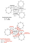 |
Fig. 1 Averaged expansion rate during the evolution of an inhomogeneous universe. Top: reversible evolution with expansion and compression modes. Down: irreversible evolution when compression modes are dissipated by virialisation through accretion shocks. |
5 Link with observations and quantitative estimates
DESI Collaboration (2024c,a) present the release of the first science data from the Dark Energy Spectroscopic Instrument (DESI) project, which includes data from commissioning and Survey Validation phases conducted between December 2020 and June 2021. The authors highlight that the DESI collaboration has successfully validated its survey design and observing strategy, ensuring the data’s quality and completeness and that future releases will facilitate detailed studies of the Universe’s large-scale structure, providing critical insights into dark energy and the fundamental physics governing the Universe’s evolution. Following the initial data release, the DESI collaboration has unveiled its first-year analysis results of baryon acoustic oscillations based on extensive observations of galaxies, quasars, and the Lyman-α forest (DESI Collaboration 2024b). While the DESI data alone align with the Λ cold dark matter (CDM) model, the results deviate when generalised to the ω0ωaCDM model. The DESI data combined with cosmic microwave background (CMB) and supernova data suggest a rejection of the ΛCDM model in favour of the ω0ωaCDM model with significant confidence levels between 2 and 4σ (DESI Collaboration 2024b). The combined data indicate a preference for ω0 > −1 and ωa < 0, where ω(a) = ω0 + ωa(1 − a) represents the equation-of-state parameter of dark energy with a(t) the scale factor of the FLRW cosmology. If confirmed, these findings could have profound implications for our understanding of the Universe’s dynamics. In that context, Tada & Terada (2024) suggest that the nature of dark energy might be explained by a quintessential scalar field, although this field could potentially become a phantom in the past. They conclude that the DESI data challenge the ΛCDM model and supports a dynamic dark energy scenario, thereby contributing to our understanding of cosmic acceleration and the potential need for new physics beyond the standard cosmological model.
However, due to the covariance of general relativity, the current approach in the standard cosmological model can be reformulated as follows: the choice of an expanding background coordinate system should be arbitrary and introducing a cosmological constant to drive the dynamics of the coordinate system has no physical meaning other than selecting an expanding coordinate system with aeff(t), Heff(t), and three velocities ueff,g for time-like geodesics such that ⟨θ⟩ ≈ 3Heff and ⟨∇ · ueff,g⟩ ≈ 0. This choice compensates for the averaged expansion rate along time-like geodesics in the coordinate system. If one prefers to use the FLRW solution of a fictive homogeneous universe without a cosmological constant, where the Hubble expansion rate is H(t) (with ![Mathematical equation: $\[H^2=8 \pi G \bar{\rho} / 3\]$](/articles/aa/full_html/2024/09/aa50818-24/aa50818-24-eq58.png) ), and the three velocities for time-like geodesics are ug, then ⟨θ⟩ = 3H + ⟨∇ · ug⟩ and ⟨∇ · ug⟩ ≠ 0 as soon as virialisation and entropy production occur. We highlight that virialisation during structure formation is likely to replace dark energy because it precisely mimics the counter-intuitive anti-gravity effect needed for dark energy. The dissipation of large-scale compression modes by virialisation stabilises large-scale gravitational collapse (anti-gravity) while remaining a purely gravitational effect, as virialised dark matter continues to be in freefall.
), and the three velocities for time-like geodesics are ug, then ⟨θ⟩ = 3H + ⟨∇ · ug⟩ and ⟨∇ · ug⟩ ≠ 0 as soon as virialisation and entropy production occur. We highlight that virialisation during structure formation is likely to replace dark energy because it precisely mimics the counter-intuitive anti-gravity effect needed for dark energy. The dissipation of large-scale compression modes by virialisation stabilises large-scale gravitational collapse (anti-gravity) while remaining a purely gravitational effect, as virialised dark matter continues to be in freefall.
In this effective coordinate system, we can use the second principle of thermodynamics to infer an effective evolution equation that takes into account entropy production,
![Mathematical equation: $\[\begin{aligned}\frac{d\left(\log V_{\mathrm{eff}}\right)}{d t} & =\frac{d\left(\log V_{\mathrm{rev}}\right)}{d t}+\frac{1}{Z k_b} \frac{d s}{d t}, \\H_{\mathrm{eff}}(t) & =H(t)+\frac{1}{3 Z k_b} \frac{d s}{d t},\end{aligned}\]$](/articles/aa/full_html/2024/09/aa50818-24/aa50818-24-eq59.png) (37)
(37)
which can be rewritten as
![Mathematical equation: $\[\begin{aligned}H_{\mathrm{eff}}(t)^2 & =\frac{8 \pi G \bar{\rho}}{3}+\frac{\Lambda_{\mathrm{eff}}(t) c^2}{3}, \\\Lambda_{\mathrm{eff}}(t) & =\frac{2 H}{c^2 Z k_b} \frac{d s}{d t}+\frac{1}{3 c^2 Z^2 k_b^2}\left(\frac{d s}{d t}\right)^2.\end{aligned}\]$](/articles/aa/full_html/2024/09/aa50818-24/aa50818-24-eq60.png) (38)
(38)
In this context, the effective cosmological constant appears to vary with time, as suggested by the early DESI data release. It is important to note, however, that this does not imply the existence of new physics; rather, the effective cosmological constant serves as a proxy to account for the impact of entropy production on the averaged expansion rate along time-like geodesics. Entropy production is expected to begin during structure formation at the first shell crossing, peak during the virialisation of structures, and gradually decline to the present day. This behaviour could simulate the need for ω(a) < −1 in the past and ω(a) > −1 in the present. As noted in Tada & Terada (2024), The increase in ω(a) is correlated with the decrease in the Hubble constant, which is the opposite direction to solve the Hubble tension. The Hubble Tension refers to the significant discrepancy between two different methods of measuring the Hubble constant. The first method involves local measurements, such as observing the distances and redshifts of nearby galaxies. The second method involves the CMB and large-scale structure data, which rely on ΛCDM model and measurements from the early Universe (Kamionkowski & Riess 2023). The local measurements consistently yield a higher value for the Hubble constant (around 73 km/s/Mpc) compared to the CMB-based measurements (around 67 km/s/Mpc). Although the decline phase of entropy production after the virialisation of structures cannot explain the Hubble tension, the initial increase phase after the first shell crossing could play an important role in resolving the current tension. However, precise estimates of the evolution of Λeff(t) require dedicated numerical simulations to accurately constrain the evolution of entropy production during structure formation and subsequent evolution.
We can, however, use existing numerical simulations to provide a more quantitative order-of-magnitude estimate. We considered the illustrative example depicted in the top panel of Fig. 2. In this scenario, we assumed that within the bound and virialised large-scale structures with a characteristic size of dlss, the local volume expansion rate, denoted as θ, is approximately negligible (θ ≈ 0). Conversely, in the expanding cosmic voids with a typical size of dvoid, θ is substantially higher, with θ ≈ 6upre–shock/dvoid ≫ 3H. The bottom panel of Fig. 2 shows an equivalent apparent velocity profile by integrating the gradients along the line of sight. Both profiles in Fig. 2 provide the same integrated redshift using Eq. (19) and illustrate how peculiar velocities resulting from structure formation can mimic a Hubble flow. Without discontinuities in Fig. 2, the velocity field divergence in the structures and in the voids would exactly compensates for one another such that ⟨∇ · ug⟩ = 0. However, this is not the case with discontinuities: in the extreme case for which ∇ · ug is strictly positive everywhere (i.e. with expanding motions in the lss regions in Fig. 2), ⟨∇ · ug⟩ is clearly strictly positive on average. In a realistic configuration for the large-scale structures with θ ≈ 0, the dominant contributor to the redshift arises from the expansion occurring within the voids, accounting for a fraction of dvoid/(dlss + dvoid). This expansion in the voids cannot be counterbalanced by compression within the structures, as it has dissipated due to violent relaxation and virialisation processes. Assuming typical structure sizes of approximately dlss ≈ 3 Mpc and void sizes around dvoid ≈ 30 Mpc, the average expansion rate, represented by ⟨θ⟩/3, attains values of the order of 70 km/s/Mpc with pre-shock velocities of roughly upre–shock ≈ 1200 km/s. This estimation falls within the same order of magnitude as the infall velocities observed in N-body numerical simulations (Zu & Weinberg 2013).
The forthcoming generation of high-resolution cosmological simulations on exascale supercomputers will be essential in advancing our understanding of entropy production through caustics (i.e. velocity discontinuities or non-collisional shocks). These simulations will enable more precise estimates of the averaged local expansion rate along time-like geodesics. Such estimates are crucial for interpreting dynamic dark energy scenarios, where dark energy could be replaced by entropy production during structure formation. These insights will be essential for analysing future data releases from the DESI collaboration and for interpreting observations from the Euclid satellite (Amendola et al. 2018). By combining Euclid’s weak lensing data, redshift surveys (including baryon acoustic oscillations, redshift distortions, and the full power spectrum shape), and CMB data from Planck, we can constrain dynamic dark energy scenarios more effectively.
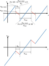 |
Fig. 2 Impact of discontinuities on a velocity profile. Top: illustration of a discontinuous velocity profile that impacts the redshift-distance relation. Bottom: equivalent apparent velocity profile derived via the integration of the gradients along the line of sight. |
6 Conclusions
This paper highlights the intricate relationship between the cosmological redshift and entropy production due to structure formation. We emphasise the need for the covariant calculation of the cosmological redshift, which accounts for peculiar motions with a local expansion rate along time-like geodesics.
Our analysis suggests that virialisation and the subsequent entropy production during structure formation play a crucial role in this dynamic. The time-varying nature of the effective cosmological constant, as indicated by recent DESI data, may be a manifestation of these processes rather than new physics. This perspective necessitates a reassessment of dark energy models, and we propose that what is currently attributed to dark energy might instead be the result of entropy production during structure formation.
Future high-resolution cosmological simulations on exascale supercomputers will be vital for refining our understanding of these phenomena. These simulations will help produce more accurate estimates of the averaged local expansion rate along time-like geodesics, providing essential insights for interpreting dynamic dark energy scenarios and forthcoming observational data from DESI and the Euclid satellite. This research opens new avenues for understanding the fundamental forces shaping our Universe, emphasising the need for continuous advancements in computational and observational cosmology.
Acknowledgements
We thank Quentin Vigneron, Thomas Guillet, and Pascal Wang for all the discussions that lead to this paper. We also thank David Elbaz and Matthias González for helpful comments on this manuscript.
References
- Amendola, L., Appleby, S., Avgoustidis, A., et al. 2018, Living Rev. Relativ., 21, 2 [NASA ADS] [CrossRef] [Google Scholar]
- Buchert, T. 2008, Gen. Relativ. Grav., 40, 467 [NASA ADS] [CrossRef] [Google Scholar]
- Buchert, T., & Ehlers, J. 1997, A&A, 320, 1 [NASA ADS] [Google Scholar]
- Buchert, T., Carfora, M., Ellis, G. F. R., et al. 2015, Class. Quant. Grav., 32, 215021 [NASA ADS] [CrossRef] [Google Scholar]
- Bunn, E. F., & Hogg, D. W. 2009, Am. J. Phys., 77, 688 [NASA ADS] [CrossRef] [Google Scholar]
- Chodorowski, M. J. 2007, MNRAS, 378, 239 [CrossRef] [Google Scholar]
- DESI Collaboration (Adame, A. G., et al.) 2024a, AJ, 167, 62 [NASA ADS] [CrossRef] [Google Scholar]
- DESI Collaboration (Adame, A. G., et al.) 2024b, arXiv e-prints [arXiv:2404.03002] [Google Scholar]
- DESI Collaboration (Adame, A. G., et al.) 2024c, AJ, 168, 58 [NASA ADS] [CrossRef] [Google Scholar]
- Després, B. 2017, Numerical Methods for Eulerian and Lagrangian Conservation Laws, Frontiers in Mathematics (Springer International Publishing) [CrossRef] [Google Scholar]
- Eisenstein, D. J., Loeb, A., & Turner, E. L. 1997, ApJ, 475, 421 [NASA ADS] [CrossRef] [Google Scholar]
- Godlewski, E., & Raviart, P. 1996, Numerical Approximation of Hyperbolic Systems of Conservation Laws, Applied Mathematical Sciences No. 118 (Springer) [CrossRef] [Google Scholar]
- Haider, M., Steinhauser, D., Vogelsberger, M., et al. 2016, MNRAS, 457, 3024 [Google Scholar]
- Ishibashi, A., & Wald, R. M. 2006, Class. Quant. Grav., 23, 235 [NASA ADS] [CrossRef] [Google Scholar]
- Kamionkowski, M., & Riess, A. G. 2023, Annu. Rev. Nucl. Part. Sci., 73, 153 [NASA ADS] [CrossRef] [Google Scholar]
- Lasky, P. D., & Lun, A. W. C. 2006, PRD, 74, 084013 [NASA ADS] [CrossRef] [Google Scholar]
- Parks, G. K., Lee, E., McCarthy, M., et al. 2012, PRL, 108, 061102 [NASA ADS] [CrossRef] [Google Scholar]
- Parks, G. K., Lee, E., Fu, S. Y., et al. 2017, Rev. Mod. Plasma Phys., 1, 1 [NASA ADS] [CrossRef] [Google Scholar]
- Peacock, J. A. 1998, Cosmological Physics (Cambridge University Press) [CrossRef] [Google Scholar]
- Peacock, J. A. 2008, A diatribe on expanding space [Google Scholar]
- Peebles, P. 1993, Principles of Physical Cosmology, Princeton Series in Physics (Princeton University Press) [Google Scholar]
- Räsänen, S. 2009, JCAP, 2009, 011 [Google Scholar]
- Rasanen, S. 2010, J. Cosm. Astropart. Phys., 2010 [Google Scholar]
- Roukema, B. F. 2018, A&A, 610, A51 [NASA ADS] [CrossRef] [EDP Sciences] [Google Scholar]
- Roukema, B. F., Ostrowski, J. J., & Buchert, T. 2013, JCAP, 2013, 043 [CrossRef] [Google Scholar]
- Tada, Y., & Terada, T. 2024, Phys. Rev. D, 109, L121305 [CrossRef] [Google Scholar]
- Tremblin, P., Chabrier, G., Padioleau, T., & Daley-Yates, S. 2022, A&A, 659, A108 [NASA ADS] [CrossRef] [EDP Sciences] [Google Scholar]
- White, S. D. M. 1996, in Gravitational Dynamics, eds. O. Lahav, E. Terlevich, & R. J. Terlevich, 121 [Google Scholar]
- Whiting, A. B. 2004, Observatory, 124, 174 [Google Scholar]
- Zu, Y., & Weinberg, D. H. 2013, MNRAS, 431, 3319 [NASA ADS] [CrossRef] [Google Scholar]
All Figures
|
Fig. 1 Averaged expansion rate during the evolution of an inhomogeneous universe. Top: reversible evolution with expansion and compression modes. Down: irreversible evolution when compression modes are dissipated by virialisation through accretion shocks. |
| In the text | |
|
Fig. 2 Impact of discontinuities on a velocity profile. Top: illustration of a discontinuous velocity profile that impacts the redshift-distance relation. Bottom: equivalent apparent velocity profile derived via the integration of the gradients along the line of sight. |
| In the text | |
Current usage metrics show cumulative count of Article Views (full-text article views including HTML views, PDF and ePub downloads, according to the available data) and Abstracts Views on Vision4Press platform.
Data correspond to usage on the plateform after 2015. The current usage metrics is available 48-96 hours after online publication and is updated daily on week days.
Initial download of the metrics may take a while.