| Issue |
A&A
Volume 689, September 2024
|
|
|---|---|---|
| Article Number | A23 | |
| Number of page(s) | 7 | |
| Section | Cosmology (including clusters of galaxies) | |
| DOI | https://doi.org/10.1051/0004-6361/202450308 | |
| Published online | 02 September 2024 | |
Energetic explosions from collisions of stars at relativistic speeds in galactic nuclei
1
Department of Physics, Harvard University, 17 Oxford Street, Cambridge, Massachusetts 02138, USA
2
Department of Astronomy, Harvard University, 60 Garden Street, Cambridge, Massachusetts 02138, USA
e-mail: This email address is being protected from spambots. You need JavaScript enabled to view it.
Received:
9
April
2024
Accepted:
3
May
2024
Abstract
Aims. We investigated collisions that could occur between stars moving near the speed of light around supermassive black holes (SMBHs) with mass M• ≳ 108 M⊙, without being tidally disrupted. Within this approximate SMBH mass range, for sun-like stars, the tidal-disruption radius is smaller than the SMBH’s event horizon; therefore we did not anticipate tidal disruption events (TDEs).
Methods. Differential collision rates were calculated by defining probability distribution functions for various parameters of interest, such as the impact parameter, distance from the SMBH at the time of the collision, the relative velocity between the two colliding stars, and the masses of the two colliding stars. The relative velocity parameter was drawn from an appropriate distribution function for SMBHs. We integrated over all these parameters to arrive at a total collision rate for a galaxy with a specific SMBH mass. We then considered how the stellar population in the vicinity of the SMBH was depleted and replenished over time, and calculated the effect this can have on the collision rate over time. We further calculated the differential collision rate as a function of the total energy released, the energy released per unit mass lost, and the galactocentric radius.
Results. The overall rate for collisions taking place within the inner ∼1 pc of galaxies with M• = 108, 109, and 1010 M⊙ are Γ ∼ 2.2 × 10⁻³, 2.2 × 10⁻⁴, and 4.7 × 10⁻⁵ yr−1, respectively. The most common collisions would release energies on the order of ∼1049 − 1051 ergs, with the energy distribution peaking at higher energies in galaxies with more massive SMBHs. In addition, we examined sample light curves for collisions with varying parameters, and find that the peak luminosity could reach or even exceed that of superluminous supernovae (SLSNe), albeit in the case of light curves with much shorter durations.
Conclusions. Weaker events may initially be mistaken for low-luminosity supernovae. In addition, we note that these events would likely create streams of debris that would accrete onto the SMBH, potentially creating accretion flares that may resemble TDEs.
Key words: black hole physics / galaxies: nuclei / galaxies: stellar content
Corresponding author; This email address is being protected from spambots. You need JavaScript enabled to view it. .
© The Authors 2024
 Open Access article, published by EDP Sciences, under the terms of the Creative Commons Attribution License (https://creativecommons.org/licenses/by/4.0), which permits unrestricted use, distribution, and reproduction in any medium, provided the original work is properly cited.
This article is published in open access under the Subscribe to Open model. This email address is being protected from spambots. You need JavaScript enabled to view it. to support open access publication.
1. Introduction
Supernova (SNe) explosions release energy on the order of 1051 ergs, originating from the runaway ignition of degenerate white dwarfs (Hillebrandt & Niemeyer 2000) or the collapse of a massive star (Woosley & Weaver 1995; Barkat et al. 1967). Rubin & Loeb (2011) and Balberg et al. (2013) considered a separate, rare explosive event resulting from collisions between hypervelocity stars in the galactic nuclei. Over time, a cluster of stars builds up in the galactic center, reaching a steady state condition in which the rate of stellar collisions is similar to the formation rate of new stars. A simplified model for the explosion light curve is Arnett’s “radiative zero” approach (Arnett 1996), which assumes that the shocked material has uniform density and temperature and a homologous velocity profile. The resulting light curve would have an average luminosity on the order of ∼2 × 1041 erg s−1, comparable to faint conventional supernovae. Furthermore, the light curve would be expected to include a long flare due to the accretion of stellar material onto the supermassive black hole (SMBH) at the center of the galaxy. Rubin & Loeb (2011) also considered mass loss from collisions between stars at the galactic center in order to constrain the stellar mass function.
In this work, we consider high-speed stars at galactic centers, where there exists a significantly higher stellar velocity dispersion (Sellgren et al. 1990). Approaching stars can be tidally disrupted by an SMBH at the tidal-disruption radius, rT ∼ R⋆(M•/M⋆)1/3, where R⋆ is the radius of the star and M• and M⋆, the masses of the black hole and the star, respectively. For Sun-like stars, the tidal-disruption radius is smaller than the black hole’s event horizon radius, rs = 2GM/c2 for black hole masses ≳108 M⊙ (Stone et al. 2019). For maximally spinning black holes, tidal disruption events (TDEs) can be observed for Sun-like stars near SMBHs with masses as high as ∼7 × 10⁸ M⊙ (Kesden 2012). Our study focused on SMBHs with masses M• ≳ 108 M⊙. It was necessary to restrict our study to these rarer, higher-mass SMBHs because we are interested in stars moving at extremely high velocities that could only be achieved very close to the center of the galaxy. At these small radii, in galaxies with lower-mass SMBHs the stars would be tidally disrupted before they could collide. Thus, our calculations centered only on galaxies where TDEs were unlikely to be observed and where a high-energy stellar collision close to the center of the galaxy could actually occur. We adopted a Newtonian approach and ignored the effects of general relativity near the SMBH because the chances of collisions occurring in a region where they would matter were extremely small.
Surveys from the last two decades such as the Sloan Digital Sky Survey (SDSS, Frieman et al. 2008), Palomar Transient Factory (PTF, Rau et al. 2009), Zwicky Transient Factory (ZTF, Bellm et al. 2014), Pan-STARRS (Scolnic et al. 2018), and others (Guillochon et al. 2017), have greatly increased the number of supernovae detected. In addition to detecting many more already well-understood classes of supernovae, previously unheard-of transients were also detected, such as superluminous supernovae (Gal-Yam 2012; Bose et al. 2018; Gal-Yam 2019), rapidly decaying supernovae (Perets et al. 2010; Kasliwal et al. 2010; Prentice et al. 2018; Nakaoka et al. 2019; Tampo et al. 2020), and transients with slow temporal evolution (Taddia et al. 2016; Arcavi et al. 2017; Dong et al. 2020; Gutiérrez et al. 2020). These discoveries have challenged existing theories of transients and suggest that a much broader range of events remain to be detected. The Vera C. Rubin Observatory is expected to start operation in 2025 and to detect hundreds of thousands of supernovae a year over a ten-year survey (Ivezić et al. 2019).
The outline of this paper is as follows: in Section 2, we describe how we simulated stellar collisions and calculated light curves. In Section 3, we provide the results of our calculations. In Section 4, we estimate the observed rates of our events. Finally, in Section 5 we summarize our main conclusions.
2. Method
2.1. Explosion parameters
Rubin & Loeb (2011) provide the differential collision rate between two species of stars, labeled “1” and “2”, at some impact parameter, b, with distribution functions f1 and f2, and velocities v1 and v2,
 (1)
(1)
This assumes spherical symmetry, with dependence only on the galocentric radius, rgal.
Adopting a power-law present-day mass function (PDMF), the equation ξ ≡ dn/dM ∝ M−α, Eq. (1) simplifies to
 (2)
(2)
The relative velocity between the stars is vrel = |v1 − v2|, and K(rgal) is a normalization constant that can be solved for from the density profile,
 (3)
(3)
The stellar density profile is adapted from Tremaine et al. (1994),
 (4)
(4)
from which we adopt the commonly used index η = 2 (Hernquist 1990), M⋆ is the total mass of the host spheroid, and rs is a distinctive scaling radius. We used the following relation between the mass of the black hole, M•, and the mass of the host spheroid, M* (Graham 2012),
 (5)
(5)
with best-fit values α = 8.4 and β = 1.01. For M• = 108, 109, and 1010 M⊙, we find spheroid masses of M⋆ ∼ 2.8 × 10¹⁰, 2.7 × 10¹¹, and 2.7 × 10¹² M⊙, respectively. Using our chosen parameters and the data from Sahu et al. (2020), we took the scaling radius to be rs ∼ 0.8, 6, and 50 kpc, respectively.
Based on Eq. (2), we defined probability distribution functions (PDFs) for the parameters b, rgal, vrel, M1, and M2. We assumed a Salpeter-like mass function and take α = 2.35, Mmin = 0.1 M⊙, and Mmax = 125 M⊙. For the impact parameter b, we take dP/db ∝ b, where we take bmin = 0 and bmax = R1 + R2, the sum of the radii of the colliding stars. This in turn requires the values of the two two radii R1 and R2. Using the stellar M − R relation,
 (6)
(6)
we assumed a = 0.026 and b = 0.945 for M < 1.66 M⊙, and a = 0.124 and b = 0.555 for M > 1.66 M⊙ (Demircan & Kahraman 1991). The PDF for the galactocentric radius, rgal, can be calculated from the density profile,  , for which we assumed rmin = 10−5 pc and rmax = 200 pc. However, the relevant range of interest for this work (i.e. where high-velocity collisions are most likely to occur) is only from approximately rmin to 1 pc. The latter distance is referred to as rcap. Tremaine et al. (1994) provided the distribution function, f1, 2,
 (7)
(7)
where Γ(x) is the gamma function, M• the mass of the SMBH, M* the stellar mass of the galaxy, and a and vg constants defined by the galaxy being studied. We were unable to find an analytical expression for the relative velocity distribution corresponding to this individual velocity distribution but were able to solve for it numerically by sampling pairs of velocities from Eq. (2) and calculating vrel as the magnitude of the difference between the two vectors (with the angles corresponding to the vectors being randomly assigned). We found that resulting histogram of vrel could be well-approximated by a Maxwellian distribution using parameters determined by a fitting function. We used this best-fit Maxwellian function as f(rgal,vrel) in our calculations, instead of a numerically-derived interpolation because we found were significantly more rapid when analytic expressions were used. We noted that the Maxwellian expression provided a slightly more conservative estimate of our final results than the numerically derived expression because it both peaked at a lower velocity for a given radius and had a less prominent high-velocity tail.
To run a Monte Carlo integration, we drew a fixed number (N = 106) of sample values from each of the probability distributions. Each sample was meant to represent two stars with known masses (M1, M2) and radii (R1, R2), colliding with some known relative velocity, vrel, and impact parameter, b, at some galactocentric radius, rgal. We used a Monte Carlo estimator to calculate the multidimensional integral,
 (8)
(8)
For a given collision, the kinetic energy of the ejecta was estimated from collision kinematics according to the following equation,
 (9)
(9)
where μ is the reduced mass and Aint(R1, R2, b) the area of intersection of the collision,
 (10)
(10)
We defined the enclosed stellar mass using,  . The mass lost in a collision between two stars could roughly be estimated to be
 (11)
(11)
where Vint(R1, R2, b) is the volume of the intersection between the two spherical stars for some impact parameters, b,
 (12)
(12)
We note that this is, at best, an order-of-magnitude approximation and that the volume fractions in Eq. (11) roughly approximate the fraction of the relative kinetic energy deposited in each star via the thermalization of shockwaves. We used this to calculate Mlost, avg ∼ 0.08 M⊙ as the average mass lost in a collision.
We note that from Eqs. (2) and (3), Γ ∝ ρ2. We can use this relation, along the stellar density profiles that were initially assumed, the resulting depletion rates, and some assumed star formation rate to calculate a basic dynamic stellar density profile that reflects stars both forming and being destroyed through collisions. For this calculation, we divided the area of interest into equal logarithmic bins in rgal. In each bin, we started with the stellar density as given by Tremaine et al. (1994), as well as the corresponding collision rate Gamma for that bin. We assumed a static star formation rate of approximately 1, 5, and 10 M⊙/yr for 108, 109, and 1010 M⊙ black hole galaxies (Behroozi et al. 2019), respectively. We further assumed that this star formation rate is uniformly distributed over the area enclosed by the galaxy’s bulge effective radius Re, which we calculated using the following M• − Re relation (Sani et al. 2011),
![Mathematical equation: $$ \begin{aligned} \log M_{\bullet }=(8.22\pm 0.08)+(0.88\pm 0.17)\times \left[\log \left(R_{\rm e}/\mathrm{kpc} \right)-0.4\right]. \end{aligned} $$](/articles/aa/full_html/2024/09/aa50308-24/aa50308-24-eq15.gif) (13)
(13)
To estimate how the stellar density will change over time, we chose a relatively small time step, such as 100 years, and then subtracted the number of stars lost to collisions and added the number of stars formed. We were then able to calculate a new value for ρ in this radius bin, and from this a new value of Γ. This process was repeated as many times as needed until a set time period had passed.
2.2. Light curves
To calculate light curves for star–star collisions, we followed the Arnett’s analytic modeling approach (Arnett 1980, 1982). This approach assumes that the ejecta is expanding homologously, that the radiation pressure dominates over gas pressure, that luminosity can be described by the spherical diffusion equation, and that the ejecta is characterized by a constant opacity (Khatami & Kasen 2019). Given these assumptions, the light curve is described by,
 (14)
(14)
where τd is the characteristic diffusion time,
![Mathematical equation: $$ \begin{aligned} \tau _d=\left[\frac{3}{4\pi }\frac{\kappa M_{\mathrm{ej} }}{v_{\mathrm{ej} }c}\frac{1}{\xi }\right]^{1/2}, \end{aligned} $$](/articles/aa/full_html/2024/09/aa50308-24/aa50308-24-eq17.gif) (15)
(15)
with Mej and vej the mass and velocity of the ejecta, respectively; κ is taken to be the electron scattering opacity κes = 0.2(1 + X) cm2/g, where X is the fractional abundance of hydrogen, and ξ = π2/3 (Khatami & Kasen 2019). Lheat(t′) is the total input heating rate, which we assumed to be Lint(t) = L0e−t/ts, normalized so that for a given collision  , where χ is an efficiency factor between 0 and 1. We estimated ts as R/tej, where R is the combined diameter of the sum of the two stars’ diameters minus the impact parameter, and given R we can calculate tej from the velocity of the ejecta, which is calculated from the kinetic energy of the explosion. In our scenario, the heat was provided early on by the kinetic energy transferred during the collision. We assumed that the heating rate decays rapidly, and that this is reflected by a very short ts. Given this, we found that the diffusion time given in Eq. (15) varies as a factor that we defined as λ,
 (16)
(16)
In our fiducial model, we assumed κ = 0.4 cm2/g, χ = 0.5, Mej = 1 M⊙, and Eej = 1051 ergs, and labelled λ with these chosen values, λ0. We note that we expect there to be an initial shock breakout which should result in a bright flash at very early times (Colgate 1974; Matzner & McKee 1999; Nakar & Sari 2010); however this feature was not included in our simplified model. Arnett’s analytical solutions were derived in the context of SNe. The flux from a SNe can be emitted in multiple wavelength regimes depending on the radioactive decay of newly synthesized isotopes. For type 1A SNe, ∼85% of the luminosity is emitted at optical wavelengths due to the radioactive decay of nickel-56 (Jha et al. 2019). In the case of stellar collisions, more detailed simulations would likely have to be conducted to precisely estimate nickel masses (Könyves-Tóth et al. 2020), especially if the heating source is more central or evenly mixed (Khatami & Kasen 2019). Additionally, γ rays may escape, and other factors could contribute to emission across various wavelength regimes.
3. Results
Using the Monte Carlo estimator method described above with N = 105 samples, we estimated total collision rates of Γ = 2.2 × 10⁻³, 2.2 × 10⁻⁴, and 4.7 × 10⁻⁵ yr−1 collisions per year for M• = 108, 109, and 1010 M⊙, respectively, in our range of interest, rgal < 1 pc. In general, although the spheroid mass is larger for galaxies with more massive SMBHs, the stellar density is overall lower, which results in a lower collision rate.
Figure 1 presents the differential collision rate binned according to both the logarithmic energy of the ejecta, Eej, and the energy per unit mass, ϵ ≡ Eej/Mlost. For the sake of comparison, we estimated the rate of core-collapse supernovae (CCSNe) in similar galaxies as the overall CCSNe volumetric rate (Frohmaier et al. 2021) normalized by the total star formation rate (SFR) and multiplied by the SFR of galaxies with SMBHs of the same mass (Behroozi et al. 2019). Using this prescription, we calculated CCSNe rates of ΓCCSNe ∼ 0.01, 0.05, and 0.1, for M• = 108, 109, and 1010, respectively. A typical CCSNe ejecta mass is on the order of Mlost ∼ 10 M⊙ (Smartt 2009). These rates are much higher than the collision rates we calculate. However, it should be noted that these CCSNe rates were calculated for entire galaxies, while we only considered the innermost ∼1 pc for stellar collisions. As a result, the CCSNe rates we mentioned should be considered overestimates for direct comparison purposes.
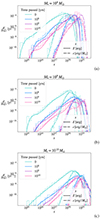 |
Fig. 1. Differential collision rate, dΓ, binned according to both the logarithmic energy of the ejecta, Eej, and the energy of the ejecta per unit mass lost, ϵ ≡ Eej/Mlost, for (a) M• = 108 M⊙, (b) M∙ = 109 M⊙, and (c) M∙ = 1010 M⊙, each for 0, 108, 109, and 1010 years passed. |
We note that although rates have been estimated, we did not compare collision events to superluminous supernovae (SLSNe), as these seem to show a preference for low-mass (low-metallicity) environments (Leloudas et al. 2015; Angus et al. 2016).
Figure 2 shows stellar density profiles for the galaxies studied with 0, 107, 108, 109, and 1010 years passed. These profiles were calculated from the differential collision rate as a function of the galactocentric radius using the profile specified in Eq. (4), which we then moved forward in time by adding stars formed during star formation and subtracting stars lost due to stellar collisions.
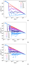 |
Fig. 2. Stellar density profiles with 0, 107, 108, 109, and 1010 years passed for (a) M• = 108 M⊙, (b) M• = 109 M⊙, and (c) M∙ = 1010 M⊙. The purpose of these profiles is to provide an idea of how stellar density profiles can change over time as the depletion of stars from collisions is balanced by the continuous formation of new stars. |
Figure 3 shows the resulting differential collision rate per logarithmic galactocentric radius, dΓ/dlnrgal, after the passage of 0, 108, 109, and 1010 years. We used the stellar density profiles calculated and shown in Fig. 2 for this purpose. We note that although dΓ ∝ ρ2 with all other variables fixed, for a given stellar density profile, the collision rate tends to decrease toward the center of the galaxy. This decrease is expected due to the overall smaller decrease in enclosed volume for smaller rgal, as the central density profiles are shallower than  as a result of their depletion. This is reflected in the
  term in Eq. (2).
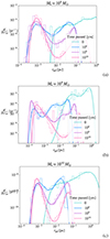 |
Fig. 3. Differential collision rate, dΓ, binned according to the logarithmic galactocentric radius, rgal, using the stellar density profiles shown in Fig. 2 for (a) M• = 108 M⊙, (b) M• = 109 M⊙, and (c) M∙ = 1010 M⊙. From Eqs. (3–4), we obtained the values for dΓ ∝ ρ2, keeping all other variables fixed. |
Figure 4 shows the distribution of the study variable  with respect to λ0 based on our fiducial model, with 0, 108, 109, and 1010 years passed. Based on this distribution, Fig. 5 shows sample light curves for six values of λ.
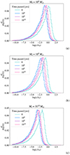 |
Fig. 4. Distribution of the variable λ with respect to λ0 following the passage of 0, 108, 109, and 1010 years for (a) M• = 108 M⊙, (b) M• = 109 M⊙, and (c) M∙ = 1010 M⊙ The majority of the samples fall within the λ/λ0 < 1 range. The long tail toward lower λ values reflects the large number of grazing impacts, which, in turn, have very low Mej. |
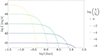 |
Fig. 5. Sample light curves based on the distribution of λ/λ0 using the analytic methods described by Arnett (1980, 1982). Although it appears possible for the peak luminosity of a stellar collision to reach or even surpass that of a SLSNe, the extremely short duration of such an event makes it less likely to be detected. However, less luminous events, which could initially be mistaken as low-luminosity supernovae, could potentially be detected, especially with advances in survey technology. |
4. Observed rates
We assumed that the volumetric rate of stellar collision events takes the following form: R(z) = R0 × f(z), where R0 is the rate at redshift zero in Mpc−3 yr−1, and f(z) is the redshift evolution. We calculated R0 as the product of the collision rate per galaxy with an SMBH of a certain mass and the volumetric density of galaxies with the same SMBH mass (Torrey et al. 2015). We associated each galaxy with an SMBH of mass M• with a halo mass, Mh, using the following approach: we calculated the bulge mass associated with M• using Eq. (2) from McConnell & Ma (2013). Next, we determined the corresponding total stellar mass using Fig. 1 in Bluck et al. (2014). Finally we estimated the corresponding halo mass using Eq. (2) in Moster et al. (2010). Given a specific halo mass, we converted the mass function fit from Warren et al. (2006) into a function of redshift, z. This involves expressing the number density of halos at a given mass as a function of redshift. We denote this function as n(z) = n0 × f(z), where n is the number density of halos at a given mass and n0 is a constant. By determining the appropriate form of the redshift evolution, f(z), we completed our calculation of R(z).
We then calculated the overall number of events of a given type by integrating over redshift using the following equation,
 (17)
(17)
where dVc/dz is the comoving volumetric element and ϵ(z) is the detection efficiency (0 ≤ ϵ(z)≤1). ϵ(z) depends on multiple factors: the survey footprint and cadence, as well as what fraction of detected events that can be distinguished. For the upcoming Large Synoptic Survey Telescope’s (LSST’s) Deep Drilling Field (DDF) survey, we expect that ϵ(z) will be no more than ∼10−3 at low redshifts (and possibly much lower due to the short duration of these events), and will decline monotonically at higher redshifts (Villar et al. 2018). It should be noted that although greater observation time will be accorded to the Wide-Fast-Deep (WFD) survey (Ivezić et al. 2019), we expect that the average revisit time of ∼3 days will be too long to identify a significant number of the events studied here, especially at higher energies.
In Fig. 6, we integrated over redshift, z, up to a certain value and plot N/ϵ as a function of z, assuming that ϵ(z) is a constant.
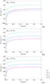 |
Fig. 6. Cumulative number of collision events for galaxies with (a) M• = 108 M⊙, (b) M• = 109 M⊙, and (c) M∙ = 1010 M⊙, for 0, 108, 109, and 1010 years passed. We made the simplifying assumption that the detection efficiencym ϵ(z), is a constant to move it out of the integral in Eq. (17) (realistically, for a survey like the LSST, we expect it to decline monotonically with redshift). |
5. Discussion
We observed that star-star collisions releasing energy in the range ∼1049 − 1051 erg are the most common in the three host galaxies we studied, with stellar masses in the range of M• = 108, 109, and 1010 M⊙. Galaxies with higher-mass SMBHs are more likely to have higher-energy collisions due to the higher velocities near the center of the galaxy, but they have overall lower collision rates due to their lower stellar density. Surveys in the near future could possibly detect several tens of events like these each year (Villar et al. 2018). In addition, collisions which release upwards of ∼1053 erg can occur with a lower collision rate ∼10−6 yr−1. These higher-energy collisions would release similar energy as SLSNe (Gal-Yam 2012), but with the distinguishing feature of being high-metallicity events due to their occurrence at the center of a galaxy (Rich et al. 2017). Conventional SLSNe, on the other hand, are believed to show a preference for low-metallicity environments (Leloudas et al. 2015; Angus et al. 2016). Furthermore, we only expect to find these high-energy, high-velocity stellar collisions in galaxies with a SMBH with mass M• ≳ 108 M⊙, which can be used as a straightforward initial screening for these events. Moreover, the most energetic collisions are most likely to occur near the SMBH, which will be an important distinguishing feature when comparing to CCSNe.
For λ/λ0 < 1, which we predict represents over half of all possible collisions, the peak luminosity is roughly equal to or even greater than that from most supernovae. However, the light curve is expected to decay much faster. At the most extreme values of λ among our samples, the light curve could have a peak luminosity roughly equal to that of a SLSNe (Gal-Yam 2019), but it would decay over six order of magnitude in luminosity in under two days, making events like these highly unlikely to be detected. However, some of the most common events we predict, with λ/λ0 ∼ 0.1 − 1, could possibly decay slowly enough to be detected. It is possible that they would also be mistaken as low-luminosity supernovae (Zampieri et al. 2003; Pastorello et al. 2004).
Finally, we note that stellar collisions are likely to create a stream of debris that would partially accrete onto the SMBH, resulting in an accretion flare. This accretion flare may resemble a TDE (Loeb & Ulmer 1997; Gezari 2021; Dai et al. 2021; Mockler & Ramirez-Ruiz 2021), even though the black hole is too massive for a TDE. The stellar explosion we have described in this work will be a precursor flare to the black hole accretion flare. We expect that the center of mass of the debris from the stellar collision would follow a trajectory consistent with momentum conservation after the collision and will also spread in its rest frame following the explosion dynamics that we consider. Altogether it would resemble a stream of gas that gets thicker over time. The accretion rate on the SMBH could be super-Eddington as in the case of TDEs and make the black hole shine around or above the Eddington luminosity, LE = 1.4 × 1046 (M•/108 M⊙) erg/s. This luminosity is far larger than we calculated for the collision itself and could be much easier to detect. The details of the accretion flare will be sensitive to the distance of the collision from the SMBH and the velocities and masses upon impact. We defer the numerical and analytical study of this problem to future work (Hu & Loeb, in prep.). In addition, the radiation emitted from these collisions could contribute to the inhabitability of nearby planets, similar to the effects from SMBHs and TDEs (Chen et al. 2018; Forbes & Loeb 2018; Pacetti et al. 2020).
Acknowledgments
This work was supported by the Black Hole Initiative at Harvard University, which is funded by grants from the John Templeton Foundation and the Gordon and Betty Moore Foundation. B.H. gratefully acknowledges support from the Department of Defense National Defense Science and Engineering Graduate Fellowship.
References
- Angus, C. R., Levan, A. J., Perley, D. A., et al. 2016, MNRAS, 458, 84 [NASA ADS] [CrossRef] [Google Scholar]
- Arcavi, I., Howell, D. A., Kasen, D., et al. 2017, Nature, 551, 210 [Google Scholar]
- Arnett, W. D. 1980, ApJ, 237, 541 [Google Scholar]
- Arnett, W. D. 1982, ApJ, 253, 785 [Google Scholar]
- Arnett, D. 1996, Supernovae and Nucleosynthesis: An Investigation of the History of Matter from the Big Bang to the Present (Princeton: Princeton University Press) [Google Scholar]
- Balberg, S., Sari, R., & Loeb, A. 2013, MNRAS, 434, L26 [CrossRef] [Google Scholar]
- Barkat, Z., Rakavy, G., & Sack, N. 1967, Phys. Rev. Lett., 18, 379 [Google Scholar]
- Behroozi, P., Wechsler, R. H., Hearin, A. P., & Conroy, C. 2019, MNRAS, 488, 3143 [NASA ADS] [CrossRef] [Google Scholar]
- Bellm, E. 2014, in The Third Hot-wiring the Transient Universe Workshop, eds. P. R. Wozniak, M. J. Graham, A. A. Mahabal, & R. Seaman, 27 [Google Scholar]
- Bluck, A. F. L., Mendel, J. T., Ellison, S. L., et al. 2014, MNRAS, 441, 599 [NASA ADS] [CrossRef] [Google Scholar]
- Bose, S., Dong, S., Pastorello, A., et al. 2018, ApJ, 853, 57 [NASA ADS] [CrossRef] [Google Scholar]
- Chen, H., Forbes, J. C., & Loeb, A. 2018, ApJ, 855, L1 [CrossRef] [Google Scholar]
- Colgate, S. A. 1974, ApJ, 187, 333 [NASA ADS] [CrossRef] [Google Scholar]
- Dai, J. L., Lodato, G., & Cheng, R. 2021, Space Sci. Rev., 217, 12 [NASA ADS] [CrossRef] [Google Scholar]
- Demircan, O., & Kahraman, G. 1991, Ap&SS, 181, 313 [Google Scholar]
- Dong, Y., Valenti, S., Bostroem, K. A., et al. 2020, ApJ, 906, 56 [NASA ADS] [CrossRef] [Google Scholar]
- Forbes, J. C., & Loeb, A. 2018, MNRAS, 479, 171 [CrossRef] [Google Scholar]
- Frieman, J. A., Bassett, B., Becker, A., et al. 2008, AJ, 135, 338 [Google Scholar]
- Frohmaier, C., Angus, C. R., Vincenzi, M., et al. 2021, MNRAS, 500, 5142 [Google Scholar]
- Gal-Yam, A. 2012, Science, 337, 927 [Google Scholar]
- Gal-Yam, A. 2019, ARA&A, 57, 305 [Google Scholar]
- Gezari, S. 2021, ARA&A, 59, 21 [NASA ADS] [CrossRef] [Google Scholar]
- Graham, A. W. 2012, ApJ, 746, 113 [NASA ADS] [CrossRef] [Google Scholar]
- Guillochon, J., Parrent, J., Kelley, L. Z., & Margutti, R. 2017, ApJ, 835, 64 [Google Scholar]
- Gutiérrez, C. P., Sullivan, M., Martinez, L., et al. 2020, MNRAS, 496, 95 [CrossRef] [Google Scholar]
- Hernquist, L. 1990, ApJ, 356, 359 [Google Scholar]
- Hillebrandt, W., & Niemeyer, J. C. 2000, ARA&A, 38, 191 [Google Scholar]
- Ivezić, Ž., Kahn, S. M., Tyson, J. A., et al. 2019, ApJ, 873, 111 [Google Scholar]
- Jha, S. W., Maguire, K., & Sullivan, M. 2019, Nat. Astron., 3, 706 [NASA ADS] [CrossRef] [Google Scholar]
- Kasliwal, M. M., Kulkarni, S. R., Gal-Yam, A., et al. 2010, ApJ, 723, L98 [NASA ADS] [CrossRef] [Google Scholar]
- Kesden, M. 2012, Phys. Rev. D, 85, 024037 [NASA ADS] [CrossRef] [Google Scholar]
- Khatami, D. K., & Kasen, D. N. 2019, ApJ, 878, 56 [NASA ADS] [CrossRef] [Google Scholar]
- Könyves-Tóth, R., Vinkó, J., Ordasi, A., et al. 2020, ApJ, 892, 121 [CrossRef] [Google Scholar]
- Leloudas, G., Schulze, S., Krühler, T., et al. 2015, MNRAS, 449, 917 [NASA ADS] [CrossRef] [Google Scholar]
- Loeb, A., & Ulmer, A. 1997, ApJ, 489, 573 [Google Scholar]
- Matzner, C. D., & McKee, C. F. 1999, ApJ, 510, 379 [Google Scholar]
- McConnell, N. J., & Ma, C.-P. 2013, ApJ, 764, 184 [Google Scholar]
- Mockler, B., & Ramirez-Ruiz, E. 2021, ApJ, 906, 101 [CrossRef] [Google Scholar]
- Moster, B. P., Somerville, R. S., Maulbetsch, C., et al. 2010, ApJ, 710, 903 [Google Scholar]
- Nakaoka, T., Moriya, T. J., Tanaka, M., et al. 2019, ApJ, 875, 76 [NASA ADS] [CrossRef] [Google Scholar]
- Nakar, E., & Sari, R. 2010, ApJ, 725, 904 [NASA ADS] [CrossRef] [Google Scholar]
- Pacetti, E., Balbi, A., Lingam, M., Tombesi, F., & Perlman, E. 2020, MNRAS, 498, 3153 [NASA ADS] [CrossRef] [Google Scholar]
- Pastorello, A., Zampieri, L., Turatto, M., et al. 2004, MNRAS, 347, 74 [Google Scholar]
- Perets, H. B., Gal-Yam, A., Mazzali, P. A., et al. 2010, Nature, 465, 322 [NASA ADS] [CrossRef] [Google Scholar]
- Prentice, S. J., Maguire, K., Smartt, S. J., et al. 2018, ApJ, 865, L3 [NASA ADS] [CrossRef] [Google Scholar]
- Rau, A., Kulkarni, S. R., Law, N. M., et al. 2009, PASP, 121, 1334 [NASA ADS] [CrossRef] [Google Scholar]
- Rich, R. M., Ryde, N., Thorsbro, B., et al. 2017, AJ, 154, 239 [NASA ADS] [CrossRef] [Google Scholar]
- Rubin, D., & Loeb, A. 2011, Adv. Astron., 2011, 174105 [CrossRef] [Google Scholar]
- Sahu, N., Graham, A. W., & Davis, B. L. 2020, ApJ, 903, 97 [NASA ADS] [CrossRef] [Google Scholar]
- Sani, E., Marconi, A., Hunt, L. K., & Risaliti, G. 2011, MNRAS, 413, 1479 [NASA ADS] [CrossRef] [Google Scholar]
- Scolnic, D. M., Jones, D. O., Rest, A., et al. 2018, ApJ, 859, 101 [NASA ADS] [CrossRef] [Google Scholar]
- Sellgren, K., McGinn, M. T., Becklin, E. E., & Hall, D. N. 1990, ApJ, 359, 112 [NASA ADS] [CrossRef] [Google Scholar]
- Smartt, S. J. 2009, ARA&A, 47, 63 [NASA ADS] [CrossRef] [Google Scholar]
- Stone, N. C., Kesden, M., Cheng, R. M., & van Velzen, S. 2019, Gen. Rel. Grav., 51, 30 [NASA ADS] [CrossRef] [Google Scholar]
- Taddia, F., Sollerman, J., Fremling, C., et al. 2016, A&A, 588, A5 [NASA ADS] [CrossRef] [EDP Sciences] [Google Scholar]
- Tampo, Y., Tanaka, M., Maeda, K., et al. 2020, ApJ, 894, 27 [Google Scholar]
- Torrey, P., Wellons, S., Machado, F., et al. 2015, MNRAS, 454, 2770 [NASA ADS] [CrossRef] [Google Scholar]
- Tremaine, S., Richstone, D. O., Byun, Y.-I., et al. 1994, AJ, 107, 634 [CrossRef] [Google Scholar]
- Villar, V. A., Nicholl, M., & Berger, E. 2018, ApJ, 869, 166 [NASA ADS] [CrossRef] [Google Scholar]
- Warren, M. S., Abazajian, K., Holz, D. E., & Teodoro, L. 2006, ApJ, 646, 881 [NASA ADS] [CrossRef] [Google Scholar]
- Woosley, S. E., & Weaver, T. A. 1995, ApJS, 101, 181 [Google Scholar]
- Zampieri, L., Pastorello, A., Turatto, M., et al. 2003, MNRAS, 338, 711 [NASA ADS] [CrossRef] [Google Scholar]
All Figures
|
Fig. 1. Differential collision rate, dΓ, binned according to both the logarithmic energy of the ejecta, Eej, and the energy of the ejecta per unit mass lost, ϵ ≡ Eej/Mlost, for (a) M• = 108 M⊙, (b) M∙ = 109 M⊙, and (c) M∙ = 1010 M⊙, each for 0, 108, 109, and 1010 years passed. |
| In the text | |
|
Fig. 2. Stellar density profiles with 0, 107, 108, 109, and 1010 years passed for (a) M• = 108 M⊙, (b) M• = 109 M⊙, and (c) M∙ = 1010 M⊙. The purpose of these profiles is to provide an idea of how stellar density profiles can change over time as the depletion of stars from collisions is balanced by the continuous formation of new stars. |
| In the text | |
|
Fig. 3. Differential collision rate, dΓ, binned according to the logarithmic galactocentric radius, rgal, using the stellar density profiles shown in Fig. 2 for (a) M• = 108 M⊙, (b) M• = 109 M⊙, and (c) M∙ = 1010 M⊙. From Eqs. (3–4), we obtained the values for dΓ ∝ ρ2, keeping all other variables fixed. |
| In the text | |
|
Fig. 4. Distribution of the variable λ with respect to λ0 following the passage of 0, 108, 109, and 1010 years for (a) M• = 108 M⊙, (b) M• = 109 M⊙, and (c) M∙ = 1010 M⊙ The majority of the samples fall within the λ/λ0 < 1 range. The long tail toward lower λ values reflects the large number of grazing impacts, which, in turn, have very low Mej. |
| In the text | |
|
Fig. 5. Sample light curves based on the distribution of λ/λ0 using the analytic methods described by Arnett (1980, 1982). Although it appears possible for the peak luminosity of a stellar collision to reach or even surpass that of a SLSNe, the extremely short duration of such an event makes it less likely to be detected. However, less luminous events, which could initially be mistaken as low-luminosity supernovae, could potentially be detected, especially with advances in survey technology. |
| In the text | |
|
Fig. 6. Cumulative number of collision events for galaxies with (a) M• = 108 M⊙, (b) M• = 109 M⊙, and (c) M∙ = 1010 M⊙, for 0, 108, 109, and 1010 years passed. We made the simplifying assumption that the detection efficiencym ϵ(z), is a constant to move it out of the integral in Eq. (17) (realistically, for a survey like the LSST, we expect it to decline monotonically with redshift). |
| In the text | |
Current usage metrics show cumulative count of Article Views (full-text article views including HTML views, PDF and ePub downloads, according to the available data) and Abstracts Views on Vision4Press platform.
Data correspond to usage on the plateform after 2015. The current usage metrics is available 48-96 hours after online publication and is updated daily on week days.
Initial download of the metrics may take a while.