| Issue |
A&A
Volume 689, September 2024
|
|
|---|---|---|
| Article Number | A12 | |
| Number of page(s) | 9 | |
| Section | Astrophysical processes | |
| DOI | https://doi.org/10.1051/0004-6361/202450017 | |
| Published online | 27 August 2024 | |
Past activity of Sgr A⋆ is unlikely to affect the local cosmic-ray spectrum up to the TeV regime
1
Centre de Recherche Astrophysique de Lyon UMR5574, ENS de Lyon, Univ. Lyon1, CNRS, Université de Lyon, 69007 Lyon, France
e-mail: jeremy.fensch@ens-lyon.fr; benoit.commercon@ens-lyon.fr
2
Universität Hamburg, Hamburger Sternwarte, Gojenbergsweg 112, 21029 Hamburg, Germany
Received:
18
March
2024
Accepted:
18
May
2024
Context The presence of kiloparsec-sized bubble structures on both sides of the Galactic plane suggests active phases of Sgr A⋆, the central supermassive black hole of the Milky Way in the last 1–6 Myr. We investigated the contribution of such events to the cosmic-ray (CR) flux measured in the solar neighborhood with numerical simulations.
Aims. We evaluate whether the population of high-energy charged particles emitted by the Galactic center could be sufficient to significantly impact the CR flux measured in the solar neighborhood.
Methods. We present a set of 3D magnetohydrodynamical simulations following the anisotropic propagation of CRs in a Milky Way-like Galaxy. We followed independent populations of CRs through time. We followed CRs originating from two different source types, namely supernovae and the Galactic center. To assess the evolution of the CR flux spectrum properties, we split these populations into two independent energy groups of 100 GeV and 10 TeV.
Results. We find that the anisotropic nature of CR diffusion dramatically affects the amount of CR energy received in the solar neighborhood. The typical timescale required to observe measurable changes in the CR spectrum slope is of the order 10 Myr, largely surpassing estimated ages of the Fermi bubbles in the active galactic nuclei (AGN) jet-driven scenario.
Conclusions. We conclude that a CR outburst from the Galactic center in the last few million years is unlikely have produced any observable feature in the local CR spectrum in the TeV regime within times consistent with current estimates of the age of the Fermi bubbles.
Key words: cosmic rays / ISM: magnetic fields / Galaxy: nucleus / solar neighborhood
© The Authors 2024
 Open Access article, published by EDP Sciences, under the terms of the Creative Commons Attribution License (https://creativecommons.org/licenses/by/4.0), which permits unrestricted use, distribution, and reproduction in any medium, provided the original work is properly cited.
This article is published in open access under the Subscribe to Open model. Subscribe to A&A to support open access publication.
1. Introduction
Building a consistent description of the cosmic-ray (CR) spectrum has been a challenging theoretical task for decades. While it is well established that these relativistic charged particles are accelerated by magnetic shocks (Fermi 1949; Bell 1978; Hillas 1984; Blandford & Eichler 1987), a comprehensive understanding of the relative contributions of all these sources is still lacking. It is thought that the Galactic cosmic-rays (GCRs) dominate the overall CR population for energies below ∼1018 eV, while substructures in the CR spectrum, the so-called knees and ankle, are considered as indicators of a transition between Galactic and extragalactic CRs (Aloisio et al. 2012).
In common scenarios, GCRs find their origin in magnetic shocks produced by supernovae (SNe) remnants (Strong et al. 2007). The total thermal energy released by an such event, of order 1051 erg, is believed to be partially converted into CRs with a yield of ∼10%, and with energies of up to a few 10–100 TeV (Lagage & Cesarsky 1983).
The case for the existence of other significant CR sources within the Galaxy has recently been bolstered by the discovery of large hemispherical structures above and below the Galactic plane by the ROSAT, Fermi and eRosita space telescopes (Bland-Hawthorn & Cohen 2003; Su et al. 2010). The soft-X-ray component of these so-called Fermi bubbles (FBs) consists of spherical bright shells extending up to 14 kpc away from both sides the galactic plane. The edge of these shells seems to coincide with that of a gamma-ray component, filling its inner volume with a relatively uniform surface brightness. Two main scenarios have been put forward to explain these features: starbust-driven disk outflows (Sofue 2000) or a past activity of the central supermassive black hole (SMBH), Sgr A⋆ (Guo & Mathews 2012). Both scenarios involve a total energy injection EF of at least 1055 erg, with the energy linked to the latter scenario ranging between 1056 and 1057 erg (Guo & Mathews 2012; Yang et al. 2022). Also, hydrodynamical simulations allow constraints to be placed on their age, which is estimated to be ∼1–6 Myr for the SMBH jet-driven scenarios (Guo & Mathews 2012; Zhang & Guo 2020), and up to 50 Myr for nuclear star formation-driven bubbles (Miller & Bregman 2016). Whether or not the expanding X-ray shells and the volume-filling gamma-ray component correspond to a single event is still unclear, because accretion from the SMBH is a stochastic phenomenon that can leads to repetitive emissions of outbursts separated by time periods of as little as ∼105 yr (King & Nixon 2015).
Theoretical studies suggest that two main scenarios can be proposed to explain the observations of the FBs, where the gamma-ray emission is the result of either (i) CR protons interacting with the surrounding medium (“hadronic” model) or (ii) inverse Compton scattering by CR electrons (“leptonic” model) (Yang et al. 2012). In both cases, the event leading to the formation of the FBs is expected to have accelerated a large quantity of CRs. Whether or not this specific population of proton and electron CRs could make a significant contribution to the CR spectrum measured on Earth remains unclear. Theoretical work following the isotropic propagation of CRs in a simplified Milky Way (MW) model led the authors to conclude that only a small fraction of the assumed injected energy EF is found to be sufficient to significantly affect the CR spectrum measured in the solar neighborhood (Jaupart et al. 2018).
In the present paper, we revisit these conclusions using a realistic magnetohydrodynamical numerical model of the MW. In particular, our model includes magnetic fields and CR diffusion along the magnetic field lines. More specifically, we study the diffusion of CRs accelerated by SN remnants or by a central source (CS). The paper is organized as follows. In Sect. 2 we present our numerical setup. In Sect. 3 we present how CRs of different origin diffuse into the Galaxy for two different energies, and discuss the implications for the CR spectrum observed in the solar neighborhood. Conclusions and perspectives are presented in Sect. 4.
2. Simulations and method
2.1. Magnetohydrodynamics with anisotropic cosmic-ray diffusion
To simulate the magnetohydrodynamical evolution of an isolated MW Galaxy, we used the adaptive mesh refinement code RAMSES (Fromang et al. 2006). We used the Harten–Lax–van Leer Discontinuity (HLLD) (Miyoshi & Kusano 2005) Riemann solver to calculate the MHD flux. Computation of the CR energy density flux was performed using the implicit numerical solver introduced in Dubois & Commerçon (2016) and Dubois et al. (2019), which we modified to support several CR groups. The full system is then described by the following set of equations:
![$$ \begin{aligned}&\frac{\partial \rho }{\partial t} + \nabla \cdot [\rho \mathbf u ] = 0, \nonumber \\&\frac{\partial \rho \mathbf u }{\partial t} + \nabla \cdot \left[ \rho \mathbf u \otimes \mathbf u + P_{\text{tot}} \mathbb{I} - \frac{\mathbf{B \otimes \mathbf B }}{4 \pi } \right] = 0,\nonumber \\&\frac{\partial E_{\text{tot}}}{\partial t} + \nabla \cdot \left[ \mathbf u (E_{\text{tot}} + P_{\text{tot}}) - \frac{(\mathbf u \cdot \mathbf B )\mathbf B }{4 \pi } \right] \\&\qquad \,\,\, = -P_{\text{CR}} \nabla \cdot \mathbf u + \nabla \cdot (\mathbb{D} \nabla E_{\text{CR}}) - \mathcal{L} (\rho ,T), \nonumber \\&\frac{\partial \mathbf B }{\partial t} - \nabla \times [\mathbf u \times \mathbf B ] = 0, \nonumber \\&\frac{\partial E_{\text{CR}}}{\partial t} + \nabla \cdot (\mathbf{u E_{\text{CR}}}) = -P_{\text{CR}} \nabla \cdot \mathbf u + \nabla \cdot (\mathbb{D} \nabla E_{\text{CR}}). \nonumber \end{aligned} $$](/articles/aa/full_html/2024/09/aa50017-24/aa50017-24-eq1.gif)
Here, ρ is the gas density, u its velocity field, B is the magnetic field vector, Ptot is the total pressure including the gas pressure P = (1 − γ)E, the magnetic field pressure Pmag = B2/(8π), and the CR pressure PCR = (γCR − 1)ECR, where γ and γCR are the adiabatic index of the gas and the CR, respectively. As the CRs are considered here as a relativistic fluid, we take γCR = 4/3, while the gas is nonrelativistic and thus characterized by the index γ = 5/3. Here, E is the gas internal energy density, ECR is the CR energy density and Etot designates the total energy density, and Etot = E + 0.5ρu2 + B2/(8π)+ECR. Also, ℒ(ρ, T) is a cooling function modeling the heating and cooling processes taking place inside the ISM, and 𝔻 describes the diffusion tensor of the CR, and can be decomposed following:

where b = B /∥B∥ is the normalized magnetic field vector and D∥ is the parallel diffusion coefficient, accounting for the diffusion along magnetic field lines. D⊥ is the perpendicular diffusion coefficient, effectively taken as 10−2 × D∥, which accounts for the diffusion of CRs perpendicularly to the magnetic field lines.
2.2. Initial conditions
The initial conditions are similar to those in Renaud et al. (2013). We initially set a box of width Lbox = 120 kpc filled with an axisymmetric distribution of gas and stellar particles. Particles position and velocity distributions of the particles are calculated using the Multi-Gaussian Expansion (MGE) method (Emsellem et al. 1994), which uses a set of Gaussian functions to model the various component of the MW based on a given input, here chosen as the Besançon model (Robin et al. 2003). The magnetic field is initially seeded with a toroidal component of amplitude 1 μG.
A spherically symmetric dark matter halo is modeled by the following density profile:
with a characteristic radius rc of 2.7 kpc and up to a truncation radius at 50 kpc, using 4 × 10⁶ particles of 1.13 × 10⁵ M⊙. A pre-existing star population of 4.6 × 10¹⁰ M⊙ is modeled with 4 × 10⁶ particles of 1.15 × 10⁴ M⊙. This population is decomposed into a bulge, a spheroid and a thick and a thin disk following Renaud et al. (2013). In addition, a particle of mass 4 × 10⁶ M⊙ is located at the center of the box to model the SMBH. The gas component is modeled by an exponential profile with a radial (respectively vertical) scale length of 10 kpc (0.25 kpc) and truncation at 30 kpc (2.5 kpc), with a total mass of 5.94 × 10⁹ M⊙.
The coarsest cells have a size of 937.5 pc. We allow refinement down to 14 pc following two criteria. We refine a cell if (i) there are more than 20 particles from initial conditions or more than 2 × 10⁴ M⊙ total mass in the cell, or (ii) the local thermal Jeans length is smaller than four times the cell size (Truelove et al. 1997).
As gas and stars do not initially share the same gravitational potential, we first need to simulate a phase of “warm relaxation” for about 1 Gyr at the beginning of our simulation with no star formation and an isothermal equation of state at T = 5 × 10⁴ K so that any structure formed during the relaxation of the gas+particles system can dissipate. During this phase, instabilities lead to the formation of the asymmetric structures of the Galaxy, namely the bar and the spiral arms.
Once these structures are formed, we activate gas cooling and heating, and star formation. Gas cooling is computed via cooling tables tabulated at solar metallicity available in the public version of RAMSES, with a temperature floor of 50 K. Star formation is modeled by a density based criterion: each cell with gas density of above 1 cm−3 and colder than 2 × 10⁴ K forms stars following the Schmidt (1959) law with 10% efficiency per free-fall time. New stars have a mass of 104 M⊙.
After an additional ∼50 Myr, the star formation rate (SFR) reaches a realistic order of magnitude (i.e. around 1 M⊙/yr). The corresponding gas density and magnetic field maps are shown in Fig. 1. CRs injection from SNe is then turned on and the simulation is continued for an extra 5 Myr so that the CRs injected from the SNe have enough time to diffuse significantly. Time at the end of this phase is hereafter referred to as t = 0.
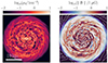 |
Fig. 1. Initial conditions for CR injection. The left panel shows the hydrogen density, while the right panel shows the magnetic field amplitude overlaid with its associated field lines. |
2.3. Stellar feedback
We include feedback from type II SNe. Injection is performed for stellar particles with an age of more than 10 Myr and a mass superior to 10 M⊙. At each injection event, mass and specific thermal energy are injected into the parent gas cell of the stellar particle following:
where m⋆ is the mass of the stellar particle, and fSNe = 0.2.
2.4. Cosmic-ray injection and diffusion
To assess the impact of a CS of CRs on the overall CR spectrum measured at the solar neighborhood, we followed the propagation of two distinct populations of CRs injected by either the SNe or the CS, each of them being split into two energy groups.
In the following, we define the solar neighborhood as the ensemble of cells of the simulation whose position fulfills −0.5 kpc < z < 0.5 kpc and 7.5 kpc < r < 8.5 kpc, where z is the axis orthogonal to the galactic disk and r is the radial position of the cell.
2.4.1. Energy groups and injection spectrum
We follow two energy groups of CRs, defined as intervals of kinetic energies following:
These groups are referred to below as either E1 or E2, or as their central value (100 GeV or 10 TeV respectively). We assume that the injection spectrum from the sources –that is, the SNe and the CS– follows a power law given by
where n(KCR) is the volumetric density of CRs, KCR is the kinetic energy of the CRs, and α is the intrinsic source injection spectrum.
For each SNe event, the amount of CR energy theoretically injected into the whole CR energy spectrum is ηSNe × eSNe, with ηSNe = 0.1 (Dermer & Powale 2013). The fractions of this energy to be injected into our two energy bins E1 and E2 is then calculated from Eq. (6), taking a slope of α = 2.4 (Lagutin et al. 2014; Blasi & Amato 2012).
We followed the same procedure for the central source. A fraction fCS = 0.1 of EF = 1056 erg, the minimum total energy required to form the FBs is assumed to be redistributed as CR energy. Note that this amount of injected CR energy can be rescaled in post-processing to explore the effect of the exact value of EF; see Sect. 3.2. The corresponding amount of energy to be injected into each energy group is obtained from the power law assuming α = 2.4, in accordance with measurements a hadronic model for the gamma-ray emission of the FBs (Ackermann et al. 2014). Several energy pulses can be injected with a fixed time interval Δt.
2.4.2. Energy losses
In this study, we only evaluate the propagation of the CRs in the Galactic disk, and not their effect on the ISM. Thus, we intentionally neglect any feedback process on the gas and any possible energy losses. In particular, we do not consider the cooling of proton CRs through pion production from proton–proton collision. The typical cooling timescale for this process is given by:
where κπ0 ≃ 0.2 is the fraction of the protons energy transferred to the pions, σpp ≃ 40 mb is the collision cross section, and nH is the hydrogen number density (Rieger 2023). Taking nH = 10 cm−3 as an upper limit for the gas density in our simulated MW, we obtain a typical cooling timescale of tpp ∼ 107 yr, which is also the typical duration of our simulations. The results presented in this paper should thus be considered as an upper limit on the contribution of the CS to the local CR population.
2.5. Simulations parameters
In total, we ran six simulations whose various parameters are summarized in Table 1. The diffusion coefficient of the CRs in the ISM for each simulation is fixed and taken assuming a power law of slope β = 0.3 (Strong et al. 2007):
Parameters of our simulations. sp and mp stands for single pulse and multiple pulses, respectively.
The obtained values for the 100 GeV and 10 TeV energy groups are 1029 cm2 s−1 and 7 × 1029 cm2 s−1, respectively. As solving the anisotropic diffusion equation of the CRs is particularly computationally expensive, our five main simulations are run with a maximum resolution of 29 pc. Two additional simulations with a maximum resolution of 15 pc and 59 pc were also run to evaluate numerical convergence. Finally, we performed one additional run with isotropic CR diffusion for comparison.
3. Results
3.1. Disk propagation and outflows
Fig. 2 presents projections of the CR energy density in both SNe and CS populations for our s15pc run and at four different times. Variable t here refers to the time since the injection of the unique pulse of 1057 erg. The 100 GeV CRs are found to diffuse much more slowly than the 10 TeV group, which is expected due to their lower diffusion coefficient. After ∼18 Myr, most 10 TeV CRs have diffused out of the Galactic center, while a large fraction of the 100 GeV CRs are still confined within the bar.
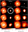 |
Fig. 2. Evolution of the several CR groups at four different times after injection of a pulse from the CS. The first and third columns present the energy density maps of the CR groups from SNe, at 100 GeV and 10 TeV respectively, while the second and fourth rows presents the same quantity for the CR groups associated with the CS. Each maps are normalized by the mean energy density in the SNe group at t = 0. The gray annulus in the second column represents the solar neighborhood as defined in the main text. (Movie available online). |
As we want to quantify the effect of CRs within the disk, we first evaluated how much of the injected energy stays within the disk and conversely what fraction of the CR energy outflows from the Galactic disk. As visible in Fig. 3, a significant amount of CR energy is propagates out of the disk, and forms large bubble-shaped structures in both sides of the Galactic plane. Remarkably, the spatial extent of these outflowing structures is consistent with the estimated size of the FBs (Su et al. 2010), which we evaluate to roughly 10 kpc at t = 3 Myr.
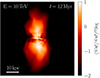 |
Fig. 3. Edge-on view of the 10 TeV CR group energy density injected by the CS in our s15pc run, 12 Myr after injection. As visible, Bubble-like structures can be seen to naturally emerge in our model due to the topology of the magnetic field. |
To evaluate the impact of the outflow on the overall CR energy budget in the disk, we introduced fi, outflow, the fraction of the energy injected by the CS escaping the disk for the energy group Ei, defined by:
with ρi, j(t) the CR energy density in cell j, for the Ei energy group and from the CS population. Vj designates the volume of the cell j. Here, the disk is defined as the set of gas cells contained in a slice 1 kpc in thickness vertically centered on the midplane of the box.
Results are shown in Fig. 4. The choice of the propagation mode is found to have minor influence on the fraction of energy staying in the disk as more than 80% of the injected CR energy escapes from the disk after at most 8 (respectively 2.5) Myr for the E1 (E2) energy bin for both anisotropic and isotropic runs. Intermittence is found to increase the proportion of energy contained in the disk, as recurrent injection from the CS constantly refuels the disk with additional energy that has not yet had time to outflow from the disk. One can verify this assumption by computing the diffusion length Ldiff after 1 Myr, the time between two consecutive pulses:
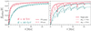 |
Fig. 4. Evolution of foutflow as a function of time and for various parameters. The left panel presents the influence of the propagation model (i.e. either anisotropic or isotropic) for our 29 pc resolution, single-pulse run (s29pc). The right panel shows the influence of the intermittence of the source. |
which is of the same order of magnitude as the half-height of the galactic disk. In any case, the CR energy escaping the disk and filling the bubble-like structures shown in Fig. 3 is expected to largely dominate the total CR energy injected by the CS. We also observe that the magnetic field topology might locally redirect outflowing streams of CRs back into the disk. However, due to the Eulerian nature of RAMSES, this effect remains difficult to quantify.
3.2. How much does the central source contribute to the local cosmic-ray population?
In Fig. 5, we evaluate the relative contribution of a single CS pulse to the total amount of CR energy measured in the solar neighborhood. Because the total energy EF required to form the FBs is not well constrained and is thought to range from 1056 to 1057 erg, we rescaled the amount of energy injected from the CS in post-processing to explore this whole interval. The resulting range of values is represented as the colored surfaces. The dotted (dashed) line corresponds to the case where EF = 1056 erg (1057 erg) is injected from the CS. The orange surface shows the estimated age τF of the FBs, which spans from 1 to 6 Myr (Guo & Mathews 2012; Zhang & Guo 2020). For each of the two energy bins, the values obtained in the case where the CRs propagate isotropically is shown by the shaded surface.
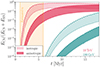 |
Fig. 5. Proportion of the total CR energy measured in the solar neighborhood attributed to the CS source as a function of time and for each energy bin. As current estimates of the energy required to form the FBs span between 1056 and 1057 erg, this quantity is left as a free parameter, the obtained range of values being represented by the colored surfaces. For each of them, the dotted (dashed) line represents the scenario in which 1056 erg (1057 erg) is required to form the FBs. The estimated age of the FBs (1–6 Myr) (Guo & Mathews 2012; Zhang & Guo 2020) is represented by the orange surface. |
In the lower-energy bin, the contribution of the CS is strictly negligible at any time in the τF estimate range. This contribution might eventually increase up to a few percent in the isotropic case after 15 Myr, much beyond the larger estimate of τF. For the higher energy bin, the contribution of the CS reaches up to a few percent within the first 6 Myr in the anisotropic case, and up to 70% in the isotropic case. We conclude that the current estimates of the age of the FBs and of the total CR energy injected from the CS imply that the CS is not able contribute significantly to the observed total CR energy budget. We note that this results from the anisotropic CR diffusion, and that considering an isotropic diffusion significantly changes the result. Taking the source intermittence into account does not change these conclusions.
We emphasize that our simulation with isotropic diffusion provides results consistent with previous theoretical work (Jaupart et al. 2018), which are thus likely to overestimate the CS contribution in the solar neighborhood by up to several orders of magnitude.
3.3. Impact on the slope of the spectrum
To assess the effect of the central source on the CR flux in the solar neighborhood, we computed the slope of the spectrum using the energy density populating our two energy bins within all the cells contained in the solar neighborhood. The configuration is illustrated in Fig. 6.
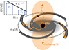 |
Fig. 6. Method used to measure the spectrum slope. The central SMBH (•) particle and the SNe (⋆) injected CRs with an initial spectrum of slope α0. While propagating along the magnetic field lines, the slope of this spectrum can exhibit some modifications due to the energy dependence of the diffusion coefficient, and to a fraction of the CRs escaping the disk. The slope of the spectrum in the solar neighborhood αS(t) (later simply denoted α) is then measured as a function of time for both the SNe and the CS populations by comparing the relative amounts of energy contained in each energy bin, averaged over all solar neighborhood gas cells. |
The slope α of the CR spectrum in the solar neighborhood (⊙) is then obtained following:
Here, the logarithmic term is the ratio between the CR energy contribution from both SNe to that from the CS contained in the solar neighborhood for the two energy bins. This fraction is obtained by summing the CR energy contained in each cell of the solar neighborhood, here labeled with the index j. The evolution of the slope is presented in Fig. 7. Here, the exact quantity of energy injected by the CS is left as a free parameter, which can vary between 1056 and 1057 erg. The colored surfaces represent the range of values covering this whole interval, while the colored lines represent the median values. The left panel shows the influence of the propagation mode on the evolution of the slope for the emission of a single pulse at t0. The gray dotted line presents the injection spectrum α0 = 2.4. The purple curve presents the slope of the CR spectrum when only accounting for the two SN groups. This slope is relatively constant, with a mean value of  , which is consistent with measured values of the average spectrum in the local Galaxy; that is, in the ISM within 1 kpc distance from the Sun (Neronov et al. 2017). The green line shows the slope of the total CR spectrum, i.e. which contains both the contribution of the SNe and the CS, for the isotropic propagation mode, while the blue line indicates the same quantity but the anisotropic propagation mode.
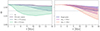 |
Fig. 7. Evolution of the spectrum slope under various conditions. Because the exact quantity of energy injected at each pulse is only weakly constrained, this quantity is left as a free parameter, which can vary between 1056 and 1057 erg. The corresponding range of values obtained are represented by the colored surfaces, while the dotted (dashed) line represents the case where a total CR energy of 1056 erg (1057 erg) is injected from the CS at t = 0. The left panel shows the influence of the propagation mode (i.e. isotropic or anisotropic). The right panel shows the influence of the source intermittence. The results of our two simulations with intermittent source, i.e. with multiple injections separated in time by period Δt are presented for Δt = 1 Myr and Δt = 3 Myr. The simulation with single anisotropic injections is also represented by the solid line for comparison. |
The propagation mode is found to have a critical impact on the ulterior shape of the spectrum. In the isotropic case, the spectrum becomes significantly harder after ∼10 Myr. This hardening effect is due to the fact that the CRs belonging to the higher energy group E2 diffuse faster than the E1 group because of their larger diffusion coefficient. They thus populate the solar neighborhood more rapidly, leading to a flattening of the spectrum. In the anisotropic case, the propagation is more sensitive to the complex morphology of the Galaxy, because the CRs propagate preferentially along magnetic field lines, which follows its spiral shape (see Fig. 1). Direct effect observed here is weaker impact on the slope of the spectrum, which is likely to be undetectable for the first 6–8 Myr after the energy injection.
We also model the eventuality that the central source of CRs is intermittent, and present the result of our two associated simulations, with injection periods of 1 Myr and 3 Myr. Results are presented in the right panel of Fig. 7. Remarkably, the latency period between the energy injection and the time at which the spectrum in the solar neighborhood starts being modified by the contribution of the CS CRs is found to be independent of the source period, and roughly equal to 6 Myr. At later times, the effect on the slope increases with the frequency of injection from the central source. About 15 Myr after the first injection, modification of the slope is found to span from ∼7% for the single-pulse simulation, to 21% for the intermittent run with Δtp = 1 Myr. Considering that current measurements of the CR spectrum slope have a precision of a few percent (Neronov et al. 2017), the contribution of the CS in the run with intermittent injection is unlikely to be measurable less than 10 Myr after the first injection. As most estimations of the age of the FBs ranges between 1 and 6 Myr, we can nevertheless conclude that a significant contribution of CRs emitted from the Galactic center to the overall CR spectrum measured in the solar neighborhood is unlikely to be observed by current surveys. These conclusions could however be modified observational evidence of an older outburst were recovered; that is, with an estimated age of more than 10 Myr.
4. Conclusion
We investigated whether or not CR outbursts from the Galactic center are likely to contribute significantly to the CR spectrum observed at the solar neighborhood. By comparing simulations run with isotropic and anisotropic diffusion, we conclude that the diffusion mode strongly influences the extent to which the CS will contribute to the local CR flux. When taking into account the preferential diffusion of CRs along magnetic field lines, CRs are found to require a much longer timescale to reach the solar neighborhood. By comparing the typical timescale required for the CRs to significantly impact the local CR flux slope with the estimated age of the Fermi-bubble in the jet-driven scenario, we conclude that the period of strong activity from the Galactic center suspected to explain the observations made by Fermi and eRosita telescopes is unlikely to affect the CR flux up to the TeV regime measured at present. Nonetheless, these conclusions do not exclude the possibility that hypothetical active phases of the Galactic center at older times contributed to the local CR spectrum.
We emphasize that both our CS injection scheme, and our propagation model remain simplified. We do not include some internal properties of the source, such as its possible anisotropy, stochasticity, or continuity. We also do not include production and acceleration of CRs within and at the edge of the outflowing bubbles, or CR reacceleration, streaming, energy loss, or secondary CR production. Further research work should focus on evaluating whether acceleration of CRs within the shock waves observed by eRosita is likely to challenge our conclusions. Treatment of CRs with a larger number of energy bins and energy losses might also help to constrain the possible effects of such an event on the local CRs flux more precisely. Finally, more observational constraints might help improving the modeling of the CS, especially regarding its intrinsic injection spectrum.
Data availability
Movie associated to Fig. 2 is available at https://www.aanda.org
Movie
Movie 1 associated with Fig. 2 (CR_total) Access here
Acknowledgments
We thank Alexandre Marcowith, Joakim Rosdahl, Yohan Dubois, Etienne Jaupart, Volker Heesen, Marcus Brüggen, Franco Vazza and Maria Werhahn for insightful discussions. We thank Eric Emsellem who provided us with the initial conditions for the Milky Way. This work was performed thanks to HPC resources provided by the PSMN (Pôle Scientifique de Modélisation Numérique) of the ENS de Lyon. We also thank Florent Renaud for providing the open-source visualization tool RDRAMSES.
References
- Ackermann, M., Albert, A., Atwood, W. B., et al. 2014, ApJ, 793, 64 [Google Scholar]
- Aloisio, R., Berezinsky, V., & Gazizov, A. 2012, Astropart. Phys., 39-40, 129 [CrossRef] [Google Scholar]
- Bell, A. R. 1978, MNRAS, 182, 147 [Google Scholar]
- Bland-Hawthorn, J., & Cohen, M. 2003, ApJ, 582, 246 [Google Scholar]
- Blandford, R., & Eichler, D. 1987, Phys. Rep., 154, 1 [Google Scholar]
- Blasi, P., & Amato, E. 2012, JCAP, 2012, 010 [CrossRef] [Google Scholar]
- Commerçon, B., Debout, V., & Teyssier, R. 2014, A&A, 563, A11 [NASA ADS] [CrossRef] [EDP Sciences] [Google Scholar]
- Dermer, C. D., & Powale, G. 2013, A&A, 553, A34 [NASA ADS] [CrossRef] [EDP Sciences] [Google Scholar]
- Dubois, Y., & Commerçon, B. 2016, A&A, 585, A138 [NASA ADS] [CrossRef] [EDP Sciences] [Google Scholar]
- Dubois, Y., Commerçon, B., Marcowith, A., & Brahimi, L. 2019, A&A, 631, A121 [NASA ADS] [CrossRef] [EDP Sciences] [Google Scholar]
- Emsellem, E., Monnet, G., & Bacon, R. 1994, A&A, 285, 723 [NASA ADS] [Google Scholar]
- Fermi, E. 1949, Phys. Rev., 75, 1169 [NASA ADS] [CrossRef] [Google Scholar]
- Fromang, S., Hennebelle, P., & Teyssier, R. 2006, A&A, 457, 371 [NASA ADS] [CrossRef] [EDP Sciences] [Google Scholar]
- Guo, F., & Mathews, W. G. 2012, ApJ, 756, 181 [NASA ADS] [CrossRef] [Google Scholar]
- Hillas, A. M. 1984, ARA&A, 22, 425 [Google Scholar]
- Jaupart, É., Parizot, É., & Allard, D. 2018, A&A, 619, A12 [NASA ADS] [CrossRef] [EDP Sciences] [Google Scholar]
- King, A., & Nixon, C. 2015, MNRAS, 453, L46 [NASA ADS] [CrossRef] [Google Scholar]
- Lagage, P. O., & Cesarsky, C. J. 1983, A&A, 125, 249 [NASA ADS] [Google Scholar]
- Lagutin, A., Tyumentsev, A., & Volkov, N. 2014, in 40th COSPAR Scientific Assembly, 40, E1.6-9-14 [NASA ADS] [Google Scholar]
- Miller, M. J., & Bregman, J. N. 2016, ApJ, 829, 9 [NASA ADS] [CrossRef] [Google Scholar]
- Miyoshi, T., & Kusano, K. 2005, J. Comput. Phys., 208, 315 [NASA ADS] [CrossRef] [Google Scholar]
- Neronov, A., Malyshev, D., & Semikoz, D. V. 2017, A&A, 606, A22 [NASA ADS] [CrossRef] [EDP Sciences] [Google Scholar]
- Renaud, F., Bournaud, F., Emsellem, E., et al. 2013, MNRAS, 436, 1836 [NASA ADS] [CrossRef] [Google Scholar]
- Rieger, F. 2023, High Energy Astrophysics ((Heidelberg Universität)) [Google Scholar]
- Robin, A. C., Reylé, C., Derrière, S., & Picaud, S. 2003, A&A, 409, 523 [NASA ADS] [CrossRef] [EDP Sciences] [Google Scholar]
- Schmidt, M. 1959, ApJ, 129, 243 [NASA ADS] [CrossRef] [Google Scholar]
- Sharma, P., & Hammett, G. W. 2007, J. Comput. Phys., 227, 123 [NASA ADS] [CrossRef] [Google Scholar]
- Sofue, Y. 2000, ApJ, 540, 224 [NASA ADS] [CrossRef] [Google Scholar]
- Strong, A. W., Moskalenko, I. V., & Ptuskin, V. S. 2007, Ann. Rev. Nucl. Part. Sci., 57, 285 [NASA ADS] [CrossRef] [Google Scholar]
- Su, M., Slatyer, T. R., & Finkbeiner, D. P. 2010, ApJ, 724, 1044 [Google Scholar]
- Truelove, J. K., Klein, R. I., McKee, C. F., et al. 1997, ApJ, 489, L179 [CrossRef] [Google Scholar]
- Yang, H. Y. K., Ruszkowski, M., Ricker, P. M., Zweibel, E., & Lee, D. 2012, ApJ, 761, 185 [NASA ADS] [CrossRef] [Google Scholar]
- Yang, H.-Y. K., Ruszkowski, M., & Zweibel, E. G. 2022, Nat. Astron., 6, 584 [NASA ADS] [CrossRef] [Google Scholar]
- Zhang, R., & Guo, F. 2020, ApJ, 894, 117 [Google Scholar]
Appendix A: Energy conservation and numerical convergence
While running our first simulations, we found nonphysical production and destruction of CR energy in our simulated box, which we associated with incorrect estimates of CR flux at interfaces between cells. Visual artifacts known as chessboard patterns are usually visible under these conditions and are shown in Fig. A.1. The origin of these patterns is discussed in Sharma & Hammett (2007).
 |
Fig. A.1. CR energy density projection for one of our preliminary, low-resolution runs. Several artifacts of diffusion produced by injection from SNe are visible. A typical feature of such events is a spike in CRs energy propagating perpendicularly to the magnetic field lines, and endowed with a chessboard pattern. |
These sources of nonconservation, known to dramatically impact the reproducibility of our results, can be efficiently reduced by the use of flux limiters. Energy conservation with and without the use of slope limiter is presented in Fig. A.2. For these tests, we theoretically injected a pulse of 1056 erg in both energy bins. Maroon and orange curves represent the energy effectively injected into the 100 GeV and the 10 TeV groups, respectively. As visible on the left panel, numerical artifacts lead to dramatic energy production, which multiplies the amount of energy theoretically injected by a factor of nearly five. After activating the slope limiter, we obtained the results presented in the right panel, which fulfill energy conservation over our tests run by nearly 90 % in both energy groups for the anisotropic runs. We verified that the subsequent energy loss, likely associated with nonconservation due to Dirichlet boundary conditions at coarse-to-fine level interface (Commerçon et al. 2014) only weakly affect our results.
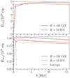 |
Fig. A.2. Comparison of energy conservation between test runs without (top panel) and with (bottom panel) flux limiter. Test runs were performed by injecting a pulse of energy 1056 erg in both energy bins at t = 0 Myr. The total CR energy contained in the simulated box is measured at various times for each of the two energy bins. |
We verified numerical convergence by running several simulations with the same physical parameters and different numerical resolutions, namely 59 pc, 29 pc, and 15 pc. In Fig. A.3, we present the total amount of energy measured in the solar neighborhood for our three single pulse simulations, with the above resolutions. While not perfectly matching, runs with resolutions of 29 pc and 15 pc seem to come to reasonable agreement. For this reason, we derived most of our results in this paper from our 29 pc resolution runs, which allowed us to run more simulations in the limited time we had for this project. We emphasize that the physical properties of our simulated Galaxy cannot be identical from one run to another. The stochasticity of star formation, as well as the resolution-dependent effect of SNe on the gas dynamics lead to star formation rates that can differ by up to ± 0.5 M⊙ yr−1 from one resolution to another. Consequently, the morphology of the Galaxy, as well as the topology of its magnetic field vary from one run to another, and can affect CR kinematics. This variability is likely to justify the lack of perfect convergence between our 29 pc and 15 pc resolution runs. Also, the amount of energy measured in the solar neighborhood in the lowest energy bin (100 GeV) is only a very small fraction of the injected energy. The dependence of the simulated Galaxy and its magnetic field on morphological properties is thus likely to be much larger than for the highest energy bin.
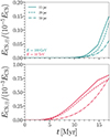 |
Fig. A.3. Numerical convergence test. A single pulse of ECS = 1056 erg is injected from the central source and the total amount of CR energy contained in the solar neighborhood cells is followed over time. |
All Tables
Parameters of our simulations. sp and mp stands for single pulse and multiple pulses, respectively.
All Figures
|
Fig. 1. Initial conditions for CR injection. The left panel shows the hydrogen density, while the right panel shows the magnetic field amplitude overlaid with its associated field lines. |
| In the text | |
|
Fig. 2. Evolution of the several CR groups at four different times after injection of a pulse from the CS. The first and third columns present the energy density maps of the CR groups from SNe, at 100 GeV and 10 TeV respectively, while the second and fourth rows presents the same quantity for the CR groups associated with the CS. Each maps are normalized by the mean energy density in the SNe group at t = 0. The gray annulus in the second column represents the solar neighborhood as defined in the main text. (Movie available online). |
| In the text | |
|
Fig. 3. Edge-on view of the 10 TeV CR group energy density injected by the CS in our s15pc run, 12 Myr after injection. As visible, Bubble-like structures can be seen to naturally emerge in our model due to the topology of the magnetic field. |
| In the text | |
|
Fig. 4. Evolution of foutflow as a function of time and for various parameters. The left panel presents the influence of the propagation model (i.e. either anisotropic or isotropic) for our 29 pc resolution, single-pulse run (s29pc). The right panel shows the influence of the intermittence of the source. |
| In the text | |
|
Fig. 5. Proportion of the total CR energy measured in the solar neighborhood attributed to the CS source as a function of time and for each energy bin. As current estimates of the energy required to form the FBs span between 1056 and 1057 erg, this quantity is left as a free parameter, the obtained range of values being represented by the colored surfaces. For each of them, the dotted (dashed) line represents the scenario in which 1056 erg (1057 erg) is required to form the FBs. The estimated age of the FBs (1–6 Myr) (Guo & Mathews 2012; Zhang & Guo 2020) is represented by the orange surface. |
| In the text | |
|
Fig. 6. Method used to measure the spectrum slope. The central SMBH (•) particle and the SNe (⋆) injected CRs with an initial spectrum of slope α0. While propagating along the magnetic field lines, the slope of this spectrum can exhibit some modifications due to the energy dependence of the diffusion coefficient, and to a fraction of the CRs escaping the disk. The slope of the spectrum in the solar neighborhood αS(t) (later simply denoted α) is then measured as a function of time for both the SNe and the CS populations by comparing the relative amounts of energy contained in each energy bin, averaged over all solar neighborhood gas cells. |
| In the text | |
|
Fig. 7. Evolution of the spectrum slope under various conditions. Because the exact quantity of energy injected at each pulse is only weakly constrained, this quantity is left as a free parameter, which can vary between 1056 and 1057 erg. The corresponding range of values obtained are represented by the colored surfaces, while the dotted (dashed) line represents the case where a total CR energy of 1056 erg (1057 erg) is injected from the CS at t = 0. The left panel shows the influence of the propagation mode (i.e. isotropic or anisotropic). The right panel shows the influence of the source intermittence. The results of our two simulations with intermittent source, i.e. with multiple injections separated in time by period Δt are presented for Δt = 1 Myr and Δt = 3 Myr. The simulation with single anisotropic injections is also represented by the solid line for comparison. |
| In the text | |
|
Fig. A.1. CR energy density projection for one of our preliminary, low-resolution runs. Several artifacts of diffusion produced by injection from SNe are visible. A typical feature of such events is a spike in CRs energy propagating perpendicularly to the magnetic field lines, and endowed with a chessboard pattern. |
| In the text | |
|
Fig. A.2. Comparison of energy conservation between test runs without (top panel) and with (bottom panel) flux limiter. Test runs were performed by injecting a pulse of energy 1056 erg in both energy bins at t = 0 Myr. The total CR energy contained in the simulated box is measured at various times for each of the two energy bins. |
| In the text | |
|
Fig. A.3. Numerical convergence test. A single pulse of ECS = 1056 erg is injected from the central source and the total amount of CR energy contained in the solar neighborhood cells is followed over time. |
| In the text | |
Current usage metrics show cumulative count of Article Views (full-text article views including HTML views, PDF and ePub downloads, according to the available data) and Abstracts Views on Vision4Press platform.
Data correspond to usage on the plateform after 2015. The current usage metrics is available 48-96 hours after online publication and is updated daily on week days.
Initial download of the metrics may take a while.