| Issue |
A&A
Volume 689, September 2024
|
|
|---|---|---|
| Article Number | A107 | |
| Number of page(s) | 18 | |
| Section | Numerical methods and codes | |
| DOI | https://doi.org/10.1051/0004-6361/202449987 | |
| Published online | 06 September 2024 | |
Low-dimensional signal representations for massive black hole binary signals analysis from LISA data
IRFU, CEA, Universite Paris-Saclay,
91191
Gif-sur-Yvette,
France
Received:
15
March
2024
Accepted:
9
June
2024
Abstract
Context. The space-based gravitational wave observatory LISA will provide a wealth of information to analyze massive black hole binaries with high chirp masses, beyond 105 solar masses. The large number of expected MBHBs (one event a day on average) increases the risk of overlapping between events. As well, the data will be contaminated with non-stationary artifacts, such as glitches and data gaps, which are expected to strongly impact the MBHB analysis, which mandates the development of dedicated detection and retrieval methods on long time intervals.
Aims. Building upon a methodological approach we introduced for galactic binaries, in this article we investigate an original non-parametric recovery of MBHB signals from measurements with instrumental noise typical of LISA in order to tackle detection and signal reconstruction tasks on long time intervals.
Methods. We investigated different approaches based on sparse signal modeling and machine learning. In this framework, we focused on recovering MBHB waveforms on long time intervals, which is a building block to further tackling more general signal recovery problems, from gap mitigation to unmixing overlapped signals. To that end, we introduced a hybrid method called SCARF (sparse chirp adaptive representation in Fourier), which combines a deep learning modeling of the merger of the MBHB with a specific adaptive time-frequency representation of the inspiral.
Results. Numerical experiments have been carried out on simulations of single MBHB events that account for the LISA response and with realistic realizations of noise. We checked the performances of the proposed hybrid method for the fast detection and recovery of the MBHB.
Key words: gravitational waves / methods: data analysis / methods: statistical
Corresponding author; This email address is being protected from spambots. You need JavaScript enabled to view it.
© The Authors 2024
 Open Access article, published by EDP Sciences, under the terms of the Creative Commons Attribution License (https://creativecommons.org/licenses/by/4.0), which permits unrestricted use, distribution, and reproduction in any medium, provided the original work is properly cited.
This article is published in open access under the Subscribe to Open model. This email address is being protected from spambots. You need JavaScript enabled to view it. to support open access publication.
1 Introduction
Space–time disturbances called gravitational waves (GWs) move at the speed of light. A wide range of phenomena, including black hole mergers, supernovae, extreme–mass ratio inspirals (EMRI), and galactic binaries (GBs), to name a few, can emit them. They are currently detectable using interferometers such as those made by the LIGO-Virgo collaboration, and in the future, owing to the Laser Interferometer Space Antenna (LISA; Amaro-Seoane et al. 2017) project run by the European Space Agency, they will be observed directly from space.
LISA is an interferometer composed of three satellites that will form three 2.5-million-kilometer-long arms. Eighteen major data streams will be produced by these three arms as time series, which will then be post-processed with time delay interferometry (TDI) to remove laser noise. The (X, Y, Z) set is the most frequent TDI combination. Since the (A, E, T) collection is designed to be statistically uncorrelated in noise, the preference in this case will be for working with a linear combination of (X, Y, Z). (For more information, check the review’s citation of Tinto & Dhurandhar 2014 and references therein).
Numerous techniques, particularly within the context of the LIGO-Virgo cooperation, have already been suggested in order to identify the gravitational signals obtained by these data channels. They cannot, however, be directly applied to the LISA mission. From the number of sources the instrument may be able to detect to their frequency range, the expected observations are in fact fundamentally different from those made by LIGO-Virgo (without even addressing the particular imprint of glitches, instrumental noise, or gaps).
Massive black hole binaries (MBHBs) are expected to be among the strongest sources measured by LISA. Detecting and extracting these signals will help answer questions regarding the supermassive black hole population models and their formation conditions (Amaro-Seoane et al. 2023), for which different hypotheses are currently considered. They are the low-frequency equivalent of the stellar origin black hole binaries detected by LIGO-Virgo. The LISA mission expects tens to a hundred detections of MBHBs each year for the duration of the mission, with signals lasting from several hours to several days, meaning an efficient extraction model is necessary to single out each of the detections and to reduce its impact on the residuals post extraction for unmixing purposes. While presenting some diversity in their waveforms, they are characterized by their “chirp”-like features, increasing in amplitude and frequency slowly at first and rapidly near coalescence, where the signal peaks before ceasing to emit altogether.
A GW signal that reaches the LISA satellite constellation will induce a signal on each of the three arms of the detector. This will yield three time series, the so-called three TDI signals X, Y, Z, sampled at time ti = i∆T (0 ≤ i < NT). It is customary to define a novel parameterization linearly A, E, and T by combining them linearly (see Tinto & Dhurandhar 2014) so that
![Mathematical equation: ${A[n] = {{{Z_i} - {X_i}} \over {\sqrt 2 }},}$](/articles/aa/full_html/2024/09/aa49987-24/aa49987-24-eq1.png) (1)
(1)
![Mathematical equation: ${E[n] = {{{Z_i} - 2{Y_i} + {X_i}} \over {\sqrt 6 }},}$](/articles/aa/full_html/2024/09/aa49987-24/aa49987-24-eq2.png) (2)
(2)
![Mathematical equation: ${T[n] = {{{Z_i} + {Y_i} + {X_i}} \over {\sqrt 3 }}.}$](/articles/aa/full_html/2024/09/aa49987-24/aa49987-24-eq3.png) (3)
(3)
Contrary to the X, Y, Z decomposition, this results in each TDI channel including measurements from all three arms. This decomposition is commonly used, as it allows for the assumption that the noise is statistically uncorrelated. In the relevant frequency range for LISA (mHz domain), the S/N of channel T is much smaller than those of the other two channels (see Prince et al. 2002). We can then neglect T and consider only the signals from A and E (Robson & Cornish 2019).
For the sake of conciseness, the measurement matrix is denoted as
 (4)
(4)
We refer to the channels A and E as UA and UE and to the measurements at time ti as Ui,A and UEi, E.
The noise is assumed to be an additive stationary Gaussian noise so that it can be described at time ti as
 (5)
(5)
where U0 is the sought-for GW signal emitted by some MBHB sources and received at time ti, and Ni stands for noise. Following Blelly et al. (2020), the noise that contaminates the LISA data is assumed to be an additive zero-mean Gaussian noise. It is further completely characterized by its power spectral density P(ν) (PSD) in the Fourier domain. In this article, the noise PSD is assumed to be known, and the measurements will be whitened and bandpass filtered as described in Appendix A.
In a context where identification relies on simplified waveforms that potentiallyrequire noticeable computing cost, it is crucial to provide fast and accurate detection and recovery algorithms that do not rely too much on parametric models. Similarly, quickly extracting all signals coming from a specific source type without identifying them presents an interest, for instance, in order to estimate the noise power spectral density or to study another type of source whose signal could be impacted by the presence of the first source type.
In the field of signal processing, the sparsity framework is particularly well adapted to deal with these questions. Sparse representations are already used in the Ligo-Virgo pipeline Coherent Waveburst (Bacon et al. 2018) to improve detection. In this pipeline, the Wilson–Daubechies–Meyer transform is applied to the measurements. This transform represents the data in a redundant wavelet dictionary, and sparsity is used to focus the signal’s power over the fewest coefficients possible in order to improve its detectability. Then this sparse representation, that is, a compact representation of the signal, is compared (using a graph) to the sparse representation of a bank of templates in order to identify it (Bammey et al. 2018). In Feng et al. (2018), the authors directly tried to recover the polarization h+, h× of GW signals. It was shown to be an efficient tool that is well adapted to the GW context. We now wish to introduce the sparsity framework to the LISA community, as it is flexible enough to deal with many of the problems that data analysis is facing today. Among these, we can mention source detection, source separation, and data gaps.
Contributions: We propose a non-parametric model for the fast detection and recovery of MBHB events from LISA data. Following Blelly et al. (2020), such a non-parametric model does not require identifying the MBHB using physical parametric models. Such surrogate models can be conveniently plugged into solvers to tackle a large span of inverse problems, such as gap mitigation (Blelly et al. 2022) or unmixing (Gertosio et al. 2023), which are relevant to a fast (pre)processing in the context of the global analysis of the LISA data. This work does not primarily focus on the low-latency alert pipeline of LISA.
In the present paper, we investigate various approaches for designing non-parametric models for MBHBs, focusing on sparse signal modeling and machine learning (ML)-based low-dimensional signal models. In the case of MBHBs, we highlight that a key challenge for designing an accurate waveform model on a long time interval is to conceive a unified model for both the spiraling and merger regime. To that end, we introduce in Sect. 3 an ML-based low-dimension representation that uses a specific autoencoder (AE) model for the merger (Sect. 2.2) and a sparse signal model that builds upon a variation of the short-term Fourier transform (STFT) for the spiraling regime (Sect. 3.1). In Sect. 4, we evaluate different non-parametric MBHB models using simulated MBHB waveforms and LISA noise as provided by the LISA Data Challenge team1. These experiments focus on assessing the detection and signal recovery efficiency of these methods.
2 Low-dimensional models for massive black hole binary detection and recovery
LISA will acquire signal through three TDI channels over several years, with each individual MBHB peaking over noise over several hours and up to several days, resulting in noisy signals. The data are further contaminated with further artifacts such as glitches or unmodeled signals. From a signal modeling perspective, MBHB waveforms can be generated through a set of a few parameters corresponding to their physical characteristics (sky location, initial phase, amplitude, chirp mass, mass ratio, spins, etc.)(Bayle 2019). A complete identification of a single MBHB signal requires accurately estimating these physical parameters. This is a particularly hard task, especially when artifacts such as gaps and/or glitches are present. Furthermore, an accurate estimation of the spiraling phase of MBHB signals on long time intervals is difficult since standard parameter estimation methods hardly capture the signal phase back in time from the merger. This is even more challenging when signals overlap with other MBHBs or when gaps or glitches are present.
In the context of fast unmixing for global analysis, it is paramount to design computationally light surrogate models for GW waveforms. To that end, in Blelly et al. (2020), we introduced a so-called non-parametric or model-free detection and recovery method for the galactic binaries. In brief, the proposed method relies on the sparse representation of GBs in the Fourier domain to distinguish between noise and signal to detect and reconstruct GB signals from noisy LISA measurements. As highlighted in Blelly et al. (2022), such models can be deployed to tackle downstream tasks such as gap mitigation.
In the spirit of Blelly et al. (2020), we propose to introduce a non-parametric method for MBHB detection and recovery from noisy LISA data. As highlighted in Sect. 1, the complexity of MBHB waveforms lies in its high non-stationary structures: (i) During the spiraling regime, MBHB waveforms are well approximated by quasi-periodic signals with a slowly increasing instantaneous frequency and amplitude. (ii) At merging time and during ringdown, the instantaneous frequency and amplitude evolve rapidly, which is akin to a transient signal. The approach we advocated in Blelly et al. (2020) strongly builds upon the use of some sparse signal representation that yields a compressed encoding of its information content. Since MBHBs have quite an inhomogeneous or non-stationary content, a single signal representation can hardly allow for an efficient sparse encoding of both the spiraling and merger/ringdown phases.
In the signal processing literature, there exist two ways to build a compressed or more generally low-dimensional representation of signals:
Sparse signal models: Sparse signal models describe signals as a sparse linear combination of signal templates, referred to as atoms. As an example, one can think of periodic or quasi-periodic signals such as GBs being sparsely represented by a few Fourier coefficients. In this framework, the sparse or low-dimensional signal representation is obtained by computing a sparse linear expansion or an expansion into the sparsifying domain. These approaches have long been popular for tackling signal detection and recovery tasks in a large variety of application domains (Potter et al. 2010; Duarte & Eldar 2011; Graff & Sidky 2015). Adpating these methods for MBHBs is discussed in Sect. 2.1.
Low-dimensional signal models: Generally speaking, signals such as MBHBs generally lie in a low-dimensional subspace or more generally on a low-dimensional manifold. Since MBHB waveforms can be described accurately from a few physical parameters, they actually belong to a low-dimensional manifold parameterized by these parameters. Low-dimensional signal models can be built using ML methods, which learn a low-dimensional encoding of the signals. A very popular ML approach is principal component analysis (PCA), which computes a linear low-dimensional signal representation in an unsupervised manner (Wold et al. 1987). More modern approaches to build non-linear low-dimensional signal models rely on models such as AEs (Hinton & Salakhutdinov 2006). This is discussed in Sect. 2.2.
2.1 Sparse signal modeling for massive black hole binaries
2.1.1 Sparse massive black hole binary representations
As noticed in the introduction, wavelets have long been used to detect and retrieve mergers of black hole binaries (Abbott et al. 2016). In this context, these approaches exploit the ability of the wavelets to sparsely or compressively represent non-stationary signals or transients, which is well suited for an MHBH merger but not for the spiraling regime of the waveform. More generally, the principle of sparse signal analysis is that a well-chosen representation yields a compressed encoding of the information contained in the signal (Tropp & Wright 2010).
As an example, we define some signal dictionary, Φ = {ϕj}, that is composed of elementary signal templates, ϕj, whose morphologies are well adapted to the signals’ structures. Somes signal U ∊ ℝN×2 can then be decomposed into the dictionary Φ as follows:
 (6)
(6)
The information content of the signal U is then encoded by c since U can be exactly reconstructed from it. The resulting representation is said to be sparse if few cj have a large amplitude while most of them have small amplitudes.
In the GW analysis literature, it is customary to resort to a time–frequency analysis by representing the data in the STFT (see Chernogor & Lazorenko 2016 for more details). In brief, a STFT performs a Fourier analysis in fixed-length time intervals. From the sparse modeling perspective, a STFT provides sparse representations for signals whose frequency varies in time slowly enough to be approximated by a periodic signal during the time interval defined in the STFT. A standard STFT with a fixed time interval yields a reasonably accurate sparse modeling of an MBHB waveform in its spiraling phase, but it is not well adapted to the merger and ringdown, which are akin to transient signals with a rapidly evolving frequency. To that respect, wavelets (Flandrin 1999) are better adapted to provide a sparse representation.
In the signal processing literature, multiscale representations such as the wavelets are standard sparse signal decompositions. In the context of GW signal analysis, wavelets constitute a robust initial decomposition to construct signal models (Bammey et al. 2018). As such, they have been used in the Waveburst detection pipeline (Klimenko et al. 2004) and as a good signal representation from which to perform Bayesian estimation of the physical parameters, as described in the Bayeswave method (Cornish & Littenberg 2015).
Next, the wavelet decomposition of some signal U is denoted as 𝒲(U). We note that the methodology does not require a specific wavelet basis to work, or even a wavelet basis at all; it only requires 𝒲(U) to be a sparse representation for U, the signal of interest. In the context of LISA, the wavelet transform of data channels A and E will be denoted as
 (7)
(7)
With the LISA noise being assumed to be additive, the measurements can be described in the wavelet domain as follows
 (8)
(8)
2.1.2 Sparse signal recovery
Sparse representations have long been used to tackle inverse problems (Elad & Aharon 2006), including for denoising and detection purposes. To that end, the signal recovery problem for a single signal, say A, is customarily addressed by solving an optimization problem of the form
 (9)
(9)
where the first term stands for the data fidelity term that measures the discrepancy between the data and the estimated signal Ā, and the second term is a regularization term that enforces a sparse solution in the wavelet domain. To that end, it is customary to define 𝒥 as the 1-norm, which is defined as the sum of the absolute value of the entries of 𝒲(Ā):
 (10)
(10)
where γ stands for the regularization parameter that allows for tuning of the trade-off between the data fidelity and the regularization terms. The solution to Eq. (10) takes the following closed-form expression:
 (11)
(11)
 (12)
(12)
where 𝒲−1 stands for the inverse wavelet transform. This solution highlights that γ acts as a threshold on the amplitude of the wavelet expansion 𝒲(A).
In the context of LISA, and following Blelly et al. (2020), the channels A and E cannot be treated independently since both are strongly correlated. Accounting for their correlation can be done by adopting a regularization term that favors common spar-sity patterns between both channels. Joint sparsity can be favored by substituting the 1-norm with the so-called 21-norm, which is defined as follows (see Nie et al. (2010) for more details):
 (13)
(13)
The signal recovery can then turn to tackling the following optimization problem:
 (14)
(14)
The solution to this problem has a closed-form expression, which can be expressed as the following soft thresholding procedure for each wavelet scale s and entry c:
 (15)
(15)
where  and
and  are the characteristic function of the set { | | 𝒲(U)s,c||2 > γ}, which takes the value of one if
  , and zero otherwise. This amounts to a thresholding operation applied to each wavelet coefficient across the channels A and E. Only the wavelet coefficients whose norm exceed γ are kept, and they are rescaled to have a 2-norm equal to 𝒲(U)s,c||2 − γ. This allows the common features between the A and E in the wavelet domain to be kept.
Tuning the regularization parameter. The regularization parameter γ plays a central role, as it allows for discriminating between the signal and the noise in the wavelet domain during the recovery process. Since the aforementioned sparse signal recovery methods lead to a thresholding procedure, tuning the threshold amounts to fixing a level under which the wavelet coefficients are considered to be noise dominated and thus rejected. Since the statistical distribution of the signal is not known, choosing the threshold is customarily tackled though a null-hypothesis testing: Under the assumption that the wavelet coefficients to be tested are distributed according to the noise distribution, the threshold is fixed with respect to a given false positive rate (Starck et al. 2010; Blelly et al. 2020).
In the present joint sparse approach for GW signal recovery, it can be highlighted in Eq. (15) that the threshold is defined with respect to the 2-norm of the wavelet coefficients across the channels. Since the data are assumed to be whitened, the noise is Gaussian, uncorrelated, and with a variance of one. Since the wavelets are orthogonal, the noise is distributed according to the same statistics in the wavelet domain. At scale , the term  s should follow a
  distribution under the null hypothesis (no signal). This entails that identifying and rejecting a noise-dominated wavelet coefficient with a certain probability, or p-value p, can be done by fixing the threshold γ from the critical value of the
  for probability p.
As highlighted in Starck et al. (2010); Blelly et al. (2020), such a thresholding procedure can lead to significantly biased solutions, especially in the high S/N regime. To overcome this limitation, two refinements have been proposed in Blelly et al. (2020):
Block thresholding (Cai 1999): The block thresholding groups of Nb consecutive coefficients in each wavelet level before applying the thresholding using critical values of a
 distribution. It relies on the fact that an MBHB signal features high local correlations in time, while noise does not and will be averaged toward zero the more coefficients are summed.
-
Re-weighted sparse regularization: The thresholding step is repeated a few times (generally two to five), with threshold values that are made dependent on the recovered signal. More precisely, the threshold γ is defined for each block Bs,i; the re-weighting scheme iteratively updates the threshold γs,i for each block. At iteration n, it is updated as follows (Blelly et al. 2020):
 (16)
(16)with κ as a parameter that controls the strength of the re-weighting. In practice, it is set to κ = 3. The threshold is not altered for coefficients whose l2-norm starts under the initial value and goes to zero the stronger the coefficients get. It has been shown in Candes et al. (2008) that this procedure provides a lower bias than standard sparsity enforcing.
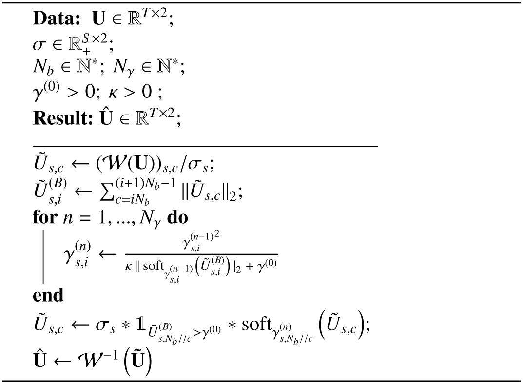
The full wavelet re-weighted block thresholding process is described in Algorithm 1, where the soft thresholding operates as described in Eq. (15). The scaling factor σ is obtained by taking the wavelet transform of a simulation of pure noise Nsim and computing a median absolute deviation (MAD) estimator on its coefficients at each wavelet level:
 (17)
(17)
where kMAD ≈ 1.48 is the scaling factor associated with a Gaus-siandistribution (see Hampel et al. 2011 forfurtherdetails onthe MAD estimator).
2.2 Machine learning for low-dimensional signal models
The physical models that describe the MBHB waveforms generally depend on a few physical parameters (Babak et al. 2020; Khan et al. 2016). From a mathematical viewpoint, the MBHB waveforms live on a low-dimensional manifold that is parameterized by the physical parameters. As advocated in the introduction, analytic non-linear parametric models are difficult and costly to use to tackle inverse problems that are relevant for LISA, such as gap mitigation. Instead, ML approaches can be adapted to be trained on approximations or surrogate models with computationally cheap inference. In contrast to sparse signal models, ML-based surrogates directly seek a joint low-dimensional model from some available training set.
In this section, we assume that we have access to some training set 𝒯 = U(j) j=1,…,T, composed of T MBHB waveforms. Each sample is composed of A and E channels with t time samples. Details about the construction of the training set are given in Sect. 4.
2.2.1 Linear unsupervised learning by principal component analysis
Principal component analysis (PCA; Wold et al. 1987) is a standard, and probably the simplest, unsupervised ML method. It allows for the building of a linear low-dimensional signal model by computing the best low-dimensional linear approximation of the training set, with respect to a quadratic approximation error. The PCA method has been shown to be quite faithful for MBHB waveform approximation about the merger (Schmidt et al. 2021), and it is quite advantageous because it can be computed by looking for the eigenvalue-eigenvector decomposition of the covariance matrix of the training set. Other approaches, such as reduced order quadrature, allow for the building of low-dimensional representations (Morrás et al. 2023); as for now, they have been limited to the acceleration of the likelihood computation for parameter estimation.
More precisely, we defined R ∊ ℝt×t as the empirical training set covariance matrix as follows:
 (18)
(18)
where  is the mean value of the j-th time sample of channel A across the training set. The eigenvalue-eigenvector decomposition of R is written as follows:
 (19)
(19)
where PR is a t × t matrix that contains the eigenvectors, and SR is a diagonal matrix whose diagonal entries are the eigenvalues that we assumed to be organized in ascending order.
For some positive integer K ≤ t, a K-dimensional linear approximation model can be computed by projecting some MHBH waveform U onto the vector space spanned by the first K eigenvectors:
![Mathematical equation: $\matrix{ {{{\bar U}_A} = {P_{\bf{R}}}[1:K]{P_{\bf{R}}}{{[1:K]}^T}{U_A}} \cr {{{\bar U}_E} = {P_{\bf{R}}}[1:K]{P_{\bf{R}}}{{[1:K]}^T}{U_E},} \cr } $](/articles/aa/full_html/2024/09/aa49987-24/aa49987-24-eq34.png) (20)
(20)
where PR[1 : K] is the submatrix of PR that is composed of its K first columns. From these equations, we could define a forward mapping Φ(U) = [PR[1 : K]TUA, PR[1 : K]TUE], which stands for the orthogonal projector onto the K-dimensional sub-space spanned by the first K principal components. Similarly, we defined a backward mapping Φ(V) = [PR[1 : K]VA, PR[1 : K] VE] that reconstructs the signal from its latent space representation V ∊ ℝK×2. The latent space dimension K enables tuning of the trade-off between noise overfitting when K is large and over-regularization for small values of K.
The choice of the value of K needs to integrate multiple parameters such as the noise level, the data dimension, and information about signal correlation. This can be done either by setting a threshold in the training correlation matrix eigenvalues (Cai et al. 2010) or by setting a compressibility level to keep a fixed dimension. The PCA method is quick and efficient as a linear dimension reduction method, but it is limited by its linear structure. It further ignores most of the physical nature of the signals modeled, only taking into account the second-order statistics of the distribution of the coefficients.
2.2.2 Autoencoder-based models
The MBHB waveforms rather leave on a non-linear low-dimensional manifold since the dependency of the waveform on the physical parameters is non-linear. This entails that linear ML approaches such as PCA are not well suited to provide an accurate low-dimensional representation of MBHB signals. In the ML literature, AEs are unsupervised neural network models, and they can be considered a non-linear generalization of the PCA (Kramer 1991). They have long been advocated as a good candidate for non-linear signal representation (Bengio et al. 2013).
More formally, an AE is defined by two non-linear mappings:
An encoder that maps the signal or direct space ℝT to the low-dimensional, so-called, latent space: Φ : ℝT → ℝk.
A decoder that maps from the latent space ℝk to ℝT :Ψ : ℝk → ℝT.
In plain English, the encoder performs a change of representation of the signal, while the decoder reconstructs it from its low-dimensional representation or latent space. Both the encoder and decoder are described by trainable parameters θ. For the sake of clarity, we do not make explicit the dependency of Φ and Ψ on θ. The elements of an AE are generally trained so as to minimize the reconstruction error in the signal space:
 (21)
(21)
Among the very large variety of AE-based models that have been proposed so far (Goodfellow et al. 2016, Chapter 14), we chose to explore the application of the interpolatory autoencoder (IAE; see Bobin et al. 2023). In contrast to the standard AE, the IAE imposes the latent space of each training sample to be described as interpolants of so-called anchorpoints, which are fixed signal examples. It has been shown that this extra constraint allows the IAE to perform quite well even when the training sample is scarce.
More formally, the IAE architecture is characterized by an extra interpolation step  in latent space. The K + 1 anchor-points are defined a priori from the training set. They are denoted by (α1,…,αK+1). As described in Bobin et al. (2023), the interpolation step consists of approximating the encoded training samples by their projection onto the affine hull of the encoded anchorpoints, as illustrated in Fig. 1.
The projection of an encoded training sample onto this affine hull of dimension K yields a barycenter of the (αi)1<i<K+1, which can be defined by its coordinates (λi)1≤i≤K+1:
 (22)
(22)
We defined Ω as the matrix formed by the encoded anchorpoints: Ω = [Φ(α1), ·⋯ , Φ(αĸ+1)] and λ = [λ1, ·⋯ , λĸ+1].
The encoder and decoder were then trained by minimizing the following training cost function:
 (23)
(23)
where the interpolation step is defined as follows:
 (24)
(24)
where 1 is a K + 1 -dimensional vector made of ones.
Different neural network architectures can be used to define the encoder and decoder, depending on the properties of the signals to be modeled. In the present article, convolutional neural networks (CNN) are used. Details of the architecture and training procedure are given in Appendix C.
Once the IAE model is trained, there exist two strategies to reconstruct an MBHB signal U0 from noisy data U:
-
Projection onto the latent space: This consists of making use of the trained encoder to project the noisy signal U onto the latent space and reconstruct the projected signal using the decoder:
 (25)
(25)Such an approach is fast, but in practice, it can lead to more biased solutions.
-
Generative model method: This approach boils down to using the decoder only as a generative or surrogate model for MBHB signals. This time, the signal is reconstructed by looking for the best parameters λ in the latent space domain so that the decoded signal minimizes the quadratic error with respect to the noisy data:
 (26)
(26)This requires minimizing a quadratic loss, which is more costly than the previous approach. However, it generally yields more accurate signal recovery, as it seeks the latent parameters that lead to the reconstruction that best fit the input signal.
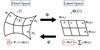 |
Fig. 1 Interpolatory autoencoder description. |
3 A hybrid approach for massive black hole binary modeling
In the previous section, we highlighted that sparse modeling is not perfectly adapted to the spiraling of MBHB waveforms for long-term modeling of these waveforms. A good sparse modeling approach would necessitate a sparse representation that can adapt to the frequency variation in the time of the spiraling period.
On the other hand, ML-based methods are good candidates for building a low-dimensional model of the coalescence, but they can hardly be used realistically on long-lasting signals since it would require learning very long time correlations. In practice, this would mean coping with very large training sets.
In order to take the best of the two approaches, we introduced a hybrid modeling of the MBHB signals:
Coalescence: At merger time, we propose modeling the waveform with a non-linear low-dimensional model. To that end, an instance of the IAE is learned.
Spiraling regime: In the spiraling regime of an MBHB signal, the waveform is oscillatory with a monotonically increasing amplitude and frequency. For that purpose, we opted for a model based on an adaptive STFT. In this framework, adaptivity comes from the dependency of the time interval decomposition on the MBHB characteristics at merger time, specifically the chirp mass.
In this section, we describe how each component of the model is built and how they are combined to yield a single model on a large time interval.
3.1 Modeling the spiraling regime of a massive black hole binary
This section introduces an adaptive time-frequency decomposition called the sparse chirp adaptive representation in Fourier (SCARF), which aims at providing an adapted time-frequency decomposition for the spiraling regime of an MBHB waveform. This decomposition is a variation of STFT with time filters of varying length to better capture the local dynamic of the chirp shape of an MBHB.
In contrast to standard time-frequency decompositions, it first builds upon a first-step processing of the coalescence, such as the IAE model described in the previous section. A specific windowed Fourier transform is then performed with a sequence of time-varying window sizes, which depend on the estimated merger. The goal of such a decomposition is to provide a time segmentation of the MBHB waveforms into time intervals in which the signal can be approximated by a quasi-periodic signal, which would consequently allow for a sparse representation in the harmonic domain. For that purpose, the windowing process must be adapted to the speed of variation of the instantaneous frequency of the waveform.
As illustrated in Fig. 2, SCARF consists of adapting both the time-frequency tiling and the analysis frequency range based on the reconstructed waveform at merger time. This yields multiple fast Fourier transforms (FFTs) on time windows of varying lengths to capture the signal at its different stages, juggling between time and frequency precision depending on its frequency shift speed. When the signal has low dynamics and is nearly stationary, long time windows are used to concentrate its power from long time samples into a few Fourier coefficients. Conversely, when the signal features higher dynamics, shorter time windows can capture the quick variations in signal frequency.
Next, the time segmentation used to build the FFT windows is a dyadic decomposition. Each segment is twice the length of the following one, with the length and position of the last segment being chosen according to the coalescence time and the system’s chirp mass, which can be estimated from the estimated signal at coalescence. This segmentation is therefore adapted to the signal’s shape and characteristic variation in frequency over time.
To counter the artifacts on the windows’ borders, short overlapping margins are integrated on both sides of each window. The decomposition is also made overcomplete by using (along the dyadic segments) the segments associated to their middles, which ensures a continuous evolution in MBHB frequencies from one window to the next. The windows are then apodized to have smooth boundaries and to overlap without loss of generalization, and they are stored in a L × T matrix:
![Mathematical equation: $W = \left[ {\matrix{ {{w_1}} \cr \vdots \cr {{w_L}} \cr } } \right] \in {^{L \times {N_T}}},$](/articles/aa/full_html/2024/09/aa49987-24/aa49987-24-eq42.png) (27)
(27)
where  are defined as Tukey apodization windows with the parameter 0 < α < 0.5 on a support determined by the time segments
 ![Mathematical equation: $\left[ {t_l^ - ,t_l^ + } \right]$](/articles/aa/full_html/2024/09/aa49987-24/aa49987-24-eq44.png) associated with the segmentation:
associated with the segmentation:
![Mathematical equation: ${w_{l,t}}{\rm{ = }}\left\{ {\matrix{ {{{\sin }^2}\left( {{{\pi \left( {t - t_l^ - } \right)} \over {2\alpha \left( {t_l^ + - t_l^ - } \right)}}} \right)\quad {\rm{ if }}t \in \left[ {t_l^ - ,t_l^ - + \alpha \left( {t_l^ + - t_l^ - } \right)} \right]} \hfill \cr {1\quad {\rm{ }}\,\,\,\,\,\,\,\,\,\,\,\,\,\,\,\,\,\,\,\,\,\,\,\,\,\,\,\,\,\,\,\,\,\,\,\,\,\,{\rm{if }}t \in \left[ {t_l^ - + \alpha \left( {t_l^ + - t_l^ - } \right),t_l^ + - \alpha \left( {t_l^ + - t_l^ - } \right)} \right]} \hfill \cr {{{\sin }^2}\left( {{{\pi \left( {t_l^ + - t} \right)} \over {2\alpha \left( {t_l^ + - t_l^ - } \right)}}} \right)\quad {\rm{ if }}t \in \left[ {t_l^ + - \alpha \left( {t_l^ + - t_l^ - } \right),t_l^ + } \right]} \hfill \cr \matrix{ {\rm{0}}\,\,\,\,\,\,\,\,\,\,\,\,\,\,\,\,\,\,\,\,\,\,\,\,\,\,\,\,\,\,\,\,\,\,\,\,\,\,\,\,\,\,\,\,\,{\rm{elsewhere}} \hfill \cr {\rm{.}} \hfill \cr} \hfill \cr } } \right.$](/articles/aa/full_html/2024/09/aa49987-24/aa49987-24-eq45.png) (28)
(28)
Then, FFTs are performed on each windowed signal cropped around ![Mathematical equation: $\left[ {t_l^ - ,t_l^ + } \right]$](/articles/aa/full_html/2024/09/aa49987-24/aa49987-24-eq46.png) , so each spectrum has a different frequency precision, depending on the length of the time segment.
, so each spectrum has a different frequency precision, depending on the length of the time segment.
The full SCARF decomposition can be described in a compact form as a single linear operator A, which from a signal x ∊ ℝT and L time segments ![Mathematical equation: ${\left( {\left[ {t_l^ - ,t_l^ + } \right]} \right)_{1 \le l \le L}}$](/articles/aa/full_html/2024/09/aa49987-24/aa49987-24-eq47.png) computes a set of L spectra, each corresponding to a different time window.
computes a set of L spectra, each corresponding to a different time window.
![Mathematical equation: ${\cal A}(U) = \left\{ {{\cal F}\left( {{{\left( {{w_l} \odot U} \right)}_{\left[ {{t_l},v_1^ + } \right]}}} \right),\quad l \in [1,L]} \right\}.$](/articles/aa/full_html/2024/09/aa49987-24/aa49987-24-eq48.png) (29)
(29)
One can define the reciprocal operator, which maps a set of spectrum associated with a given time segmentation onto a time signal – noted 𝒜⊤. This operator is obtained by taking the inverse Fourier transforms of each spectrum, zero padding according to the time segmentation, and taking the sum over the lines normalized by the sum of the windows to get a signal back in ℝT.
![Mathematical equation: ${{\cal A}^ \top }(\tilde U) = {1 \over {\sum\nolimits_i {{w_{i,t}}} }}\sum\limits_l {\left( {{{{\mathop{\rm padding}\nolimits} }_{\left. {t_l^ - ,t_l^ + } \right]}}\left( {{{\cal F}^{ - 1}}\left( {{{\tilde U}_l}} \right)} \right)} \right)} ,$](/articles/aa/full_html/2024/09/aa49987-24/aa49987-24-eq49.png) (30)
(30)
where the zero-padding operator centers the signals of different lengths on each time bin on the right time segment ![Mathematical equation: $\left[ {t_l^ - ,t_l^ + } \right]$](/articles/aa/full_html/2024/09/aa49987-24/aa49987-24-eq50.png) and creates a L × T matrix from a set of L cropped signals, see Appendix D for details. We note that the operator 𝒜⊤ is a left inverse of 𝒜; indeed, ∀x ∊ ℝT, 𝒜⊤𝒜(x) = x and the exact inverse if the time segments form a non-overlapping partition of the complete signal duration.
and creates a L × T matrix from a set of L cropped signals, see Appendix D for details. We note that the operator 𝒜⊤ is a left inverse of 𝒜; indeed, ∀x ∊ ℝT, 𝒜⊤𝒜(x) = x and the exact inverse if the time segments form a non-overlapping partition of the complete signal duration.
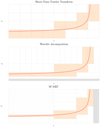 |
Fig. 2 Different time-frequency tiling strategies and their respective efficiency at capturing an MBHB signal (represented in red). In a good sparse representation, the ratio of the number of active blocks over total blocks should be small. Furthermore, to increase the S/N within blocks and improve detectability, the ratio of the signal power over the block area should be high, especially early in the inspiral, where signal power is easily drowned in noise. |
3.2 Sparse signal recovery within the SCARF domain
The SCARF decomposition is a sparse representation of MBHB signals. In this paragraph, we extend the thresholding-based denoising procedure described in Sect. 2.1.
In contrast to wavelet-based thresholding, more specific constraints can be applied to improve signal extraction using additional knowledge on the MBHB waveform characteristics:
Starting from the merger and going back in time, the MBHB waveform is a single mode signal with an instantaneous frequency that is known to be monotonically evolving. This knowledge can be enforced in the thresholding process by constraining to select only active Fourier coefficients in a set of contiguous frequencies.
The MBHB waveform further shows a monotonically decreasing instantaneous frequency. Consequently, within the SCARF domain, it is meaningful to consider the selection of the Fourier coefficients that have a frequency lower than the frequencies in the merger region and to set the others to zero.
From the monotonic decrease of the instantaneous frequency, the frequency range to be explored in the first SCARF time interval should be lower than the frequency range measured in the coalescence regime. As advocated earlier, it is then possible to benefit from the reconstructed merger by constraining the frequency range to be considered to frequencies that are lower than the one observed at the vicinity of the merger. This constraint allowed us to benefit from the MBHB recovery at higher S/N close to the merger, as it helps track the signal in lower S/N regions in the inspiral regime. Under the hypothesis that two consecutive windows wi and wi+1 overlap, this makes it possible to introduce a second constraint that iteratively provides an acceptable range of active frequencies for spectrum i depending on the active frequencies of spectrum i + 1.
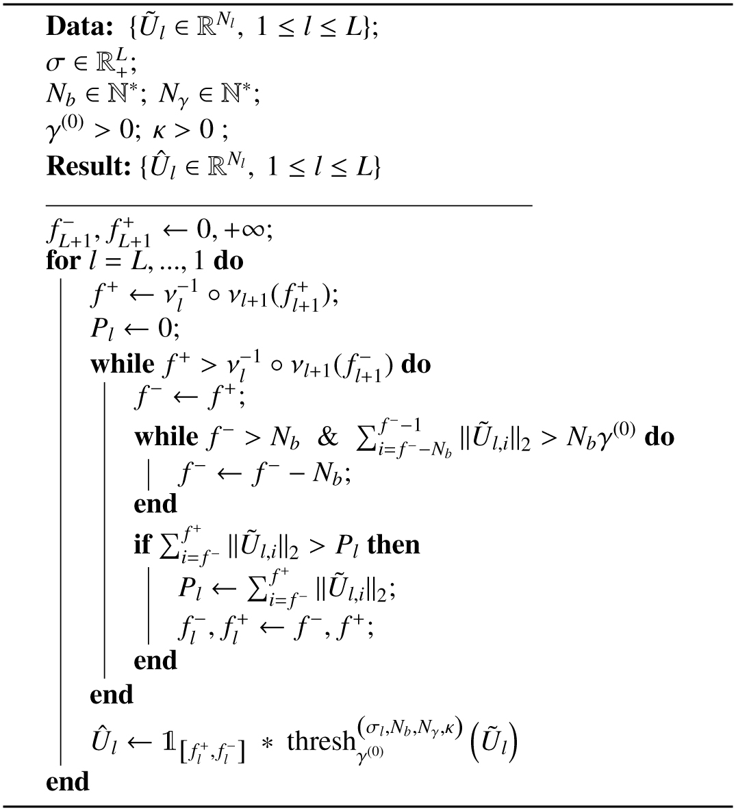
These constraints are detailed in Alg. 2 and illustrated in Fig. 3 and rely on creating for each spectrum a set of acceptable frequencies ![Mathematical equation: ${_l} = \left[ {f_l^ - ,f_l^ + } \right]$](/articles/aa/full_html/2024/09/aa49987-24/aa49987-24-eq51.png) :
:
![Mathematical equation: $\eqalign{ & \,\,\,\,\,\,\,\,\,\,\,\hat U = {{\cal A}^ \top }(\tilde U){\rm{ }} \cr & s.t.{\rm{ }}{{\tilde U}_{l,c}} = \left\{ {\matrix{ {{\rm{ thresh }}_{{\gamma ^{(0)}}}^{\left( {{\sigma _l},{N_b},{N_\gamma },k} \right)}\left( {{{\tilde U}_{l,c}}} \right)} \hfill & {{\rm{ if }}c \in \left[ {t_l^ - ,t_l^ + } \right]} \hfill \cr 0 \hfill & {{\rm{ otherwise, }}} \hfill \cr } } \right. \cr} $](/articles/aa/full_html/2024/09/aa49987-24/aa49987-24-eq52.png) (31)
(31)
where thresh  represents the re-weighted block soft-thresholding operation described in Algorithm 1.
The algorithm uses the mapping νi : ℕ → ℝ+, which translates the frequency indexes in the l-th spectrum to physical frequencies in hertz. It is necessary as each spectrum has a different frequency step size because of their varying time window lengths. The inverse operator  maps a frequency to the upper closest index associated with the absolute frequency in the spectrum l.
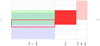 |
Fig. 3 Sketch of the SCARF time-frequency decomposition: the red block is the selected frequency segment on time bin , the candidates for time segments l – 1 are the ones with an upper bound among the green blocks, and the lower bound in the blue ones. The most powerful contiguous block are composed of elements that are each above threshold is selected as an active block on time segment l – 1 before moving back one time segment. |
4 Experimental results on simulated data
4.1 Data generation
4.1.1 Massive black hole binary signals
In the following numerical experiments, the MBHB signals were simulated using the lisabeta code (Marsat & Baker 2018) to create fast and realistic waveforms from a set of physical parameters. Details about the simulation of MBHBs are given in Appendix B. In this work, the evaluation of the different representations is limited to the modeling of the 22 modes of the MBHB waveforms with three varying parameters: the chirp mass, mass ratio, and the initial phase. A generalization to more complex models is left for future work. More precisely, we tuned the parameters as follows:
The chirp mass range was taken between 5 · 105M⊙ and 5 · 106 M⊙ by sampling a uniform on the log10 of the range of the chirp masses. This is the parameter with the strongest impact on the waveform’s shape, and in the analysis (see example in Fig. 4), the signals were separated into three bins of Mc to capture its impact on the analysis: Mc1 = [5 · 105M⊙ − 1.07 · 106M⊙], Mc2 = [1.07 · 106M⊙ − 2.32 · 106M⊙], and Mc3 = [2.32 · 106M⊙ − 5 · 106M⊙].
The mass ratio q was sampled from a uniform distribution on [1,3], which provides some variety while remaining in the MBHB regime.
The initial phase of the signal was sampled uniformly on [0, 2π].
A training set of 5000 MBHBs cropped on 3000 time samples around coalescence was generated with this method to train the IAE and the PCA.
4.1.2 Noise contamination
To generate the noise simulation, the power spectrum density (PSD), noted as PS D and provided in the LDC (with model MRDv1), was used as a diagonal correlation matrix to generate Gaussian-independent colored noise in the Fourier domain. The S/N was defined using the convention
 (32)
(32)
where j indexes the frequencies of the real FFT and c indexes the channels A and E. It was computed on the full signal, which may result in different noise levels depending on the chirp mass of the signal, which affects the signal power spreading over time. The coefficient δf denotes the frequency step in the FFT. We note that it scales linearly with the signal and that changing the frequency sampling rate multiplies both δf and PS D by the same factor. To generate a noisy MBHB signal with a given S/N, the MBHB was scaled by the factor  without modifying the noise generated by the PSD.
To illustrate this point, it is interesting to focus on low S/N, as it tests the limits of the methods to capture MBHBs near coalescence. These tests were performed on a range of S/N from five to 500. However, at such low S/N, the inspiral is very quickly drowned in noise, and we made the choice to use higher S/N MBHBs to test the capacity for inspiral recovery on longer timescales. As such, these tests were performed on MBHBs with S/N ranging from 500 to 2000.
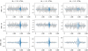 |
Fig. 4 Preprocessed (whitened and bandpassed) MBHB coalescences in time domain with noise (grey) and clean (blue) for different chirp masses and S/N. |
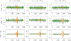 |
Fig. 5 Reconstructed signals for the different methods at multiple chirp masses and S/N. The gray signal corresponds to the noisy input, the blue one to PCA reconstruction, the green one to wavelet reconstruction, and the orange one to the IAE reconstruction. |
4.1.3 Signal pre-processing
Training and testing data were pre-processed by whitening and bandpassing them, which amounts to dividing the signal by the theoretical PSD in the Fourier domain and multiplying the result by a Butterworth filter with a frequency response:
 (33)
(33)
In practice, the cutting frequencies are set as fmin = 1 · 10−5Hɀ and fmax = 2 · 10−2Hɀ, with the filter order n = 4 to effectively cut the power out of the gravitational signal bandwidth.
4.2 Analysis methods
4.2.1 Implementation details
The details of the implementation of the different methods are listed below:
Principal component analysis – PCA: The PCA was performed on ten and 100 components to get the respective efficiency ranges of each and to compare with IAE. When not specified, the PCA with ten components is the default comparison investigated in this work; the one with 100 components was taken as an example of a different balance between data fidelity and regularization.
Interpolatory AutoEncoder 0 IAE: The IAE was performed using ten anchor points taken from the training set. The encoder and decoder were CNN composed of 12 layers. See Appendix C for details on the implementation.
Wavelets: The Daubechies wavelets from the pywavelets Python library were used on nine levels for the full signal of length 210 000, padded to 262 144 with a thresholding set at a rejection rate of 0.9 to match the rejection rate of SCARF.
SCARF: The SCARF decomposition was tested on different time segmentations built from dyadic decompositions of the full inspiral time span with different starting window positions and lengths. These decompositions were furthermore made redundant by including the segments bounded by the middle points of each dyadic segment in order to reduce the loss of quality on the intersection between successive windows. The windows associated with these segments were apodized by taking the Tuker cos squared smooth borders, with an apodization length of 10% of the full segment on each side. See Appendix D for details and illustrations on the decomposition.
4.2.2 Performance metrics
The normalized mean squared error (NMSE) was used to measure the quality of the extracted signal compared to the ground truth signal injected in the first place and was defined as
 (34)
(34)
The NMSE grows logarithmically as the mean square error of the estimation decreases, with higher NMSEs corresponding to a better reconstruction.
A sliding NMSE was used to get a local measure of error on the inspiral signals in order to block higher S/N regions close to merger from overpowering lower and earlier inspiral segments. It was computed on sliding windows of length 2000, with a striding of 100. In the presented results, the median NMSE over all the MBHB realizations is plotted, and the area between the first and third quartiles is filled.
4.3 Numerical results
4.3.1 Coalescence reconstruction
The performance on coalescence was measured by computing the NMSE on the coalescence signal. Examples of reconstruction results are featured in Fig. 5. The results presented in Fig. 6 show the evolution of the median NMSE over an S/N ranging from five to 500 for the different methods tested.
For an S/N lower than ten, all the methods had trouble reconstructing a faithful signal, with NMSE values close to zero. for an S/N larger than ten, the PCA with ten components saturates at a fixed NMSE, which is limited by the ability to accurately recover the coalescence signal from ten principal components only. The use of more components, such as 100, provided a much better NMSE, especially for S/N greater than 20, but at the cost of noise overfitting at very low S/N. Wavelets gave very similar results, with a two to three discrepancy with respect to the PCA with 100 components. The IAE significantly improved the reconstruction quality, with an NMSE gain that can reach up to 10dB, but with a tendency to saturation for S/N larger 400. Indeed as any with AE, the IAE suffers from model bias, which becomes negligible when the noise is large enough, but it can be dominant in the high S/N regime. In contrast, wavelets asymptotically provide a vanishing error when the noise vanishes since the threshold of the wavelet-based recovery process depends linearly on the noise level. Similar results can be observed in different bins of chirp mass. A small difference in performance for the highest chirp masses can be seen for learning-based methods, which is due to them being on the edge of the training sample and therefore not being completely captured by the IAE or PCA. Training the IAE required about three days on a single A100 40GB GPU. The inference took 1500s to handle 3000 waveforms of 3000 time samples on the same configuration. Meanwhile, the PCA took a few minutes to train on the same training data set using 16GB CPU and fits in a few seconds, and the wavelets took around 5 min to perform decomposition, thresholding, and recomposition. This trend is illustrated in Fig. 7, where the performance drops on the high chirp mass part of the parameter space for all the trained methods.
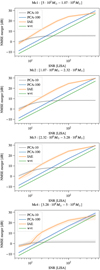 |
Fig. 6 Evolution of the median NMSE over S/N on signal extracted at merger. |
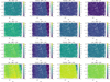 |
Fig. 7 Scatter plots of the NMSE as a function of the chirp mass and mass ratio for different methods and S/N values. |
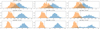 |
Fig. 8 Detection histograms for PCA (12 norm statistic measured on pure noise in orange and on noisy signal in blue). |
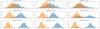 |
Fig. 9 Detection histograms for IAE (12 norm statistic measured on pure noise in orange and on noisy signal in blue). |
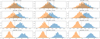 |
Fig. 10 Detection histograms for wavelets (12 norm statistic measured on pure noise in orange and on noisy signal in blue). |
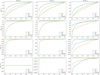 |
Fig. 11 ROC curves at different S/N and chirp masses for PCA, IAE, and wavelet detection. |
4.3.2 Detection
The methods introduced in this article can be used to detect MBHB events. For that purpose, a straightforward approach consists of taking a detection decision based on some relevant statistics with respect to a null or noise-only hypothesis.
For that purpose, the detection process is performed as follows:
Reconstruct the signal by applying one of the models described in the previous section and compute some relevant statistics. In the present paper, the l2 norm was chosen, as it computes the overall power of the detected signal.
Generate noise-only signals, apply the reconstruction step, and measure the same statistics. This enables the building of a histogram of the detection statistics in the noise-only case.
For a given probability, the detection threshold is derived from the noise-only distribution and detection is claimed based on this threshold. The detection threshold is determined by taking the inverse of the empirical cumulative density function and applying it to the detection level chosen.
In the next section, the number of noise realizations has been fixed to 1000. The threshold is set with respect to a p-value of 0.99, which amounts to a percent-level false positive rate.
To illustrate how the different methods behave, the histograms of the noise-only (orange) and signal plus noise (blue) Monte Carlo simulations for various chirp mass bins and S/N values are presented in Fig. 9 (respectively Figs. 8 and 10) for the IAE (respectively PCA and wavelets). It is important to note that the detection efficiency of a given method is related to its ability to distinguish between the noise-only distribution and the noisy signal one. Generally speaking, the more separated the two distributions are, the more efficient the methods are for detection.
The detection efficiency may further depend on the detection threshold, which could lead to different false or true positive trade-offs. To that end, it is customary to assess a detection method based on its receiver operating characteristic (ROC) curve, which features the evolution of the false positive and true positive rates when the detection thresholds evolve. The ROC curves provide a complete picture of the detection efficiency of a given method. The ROC curves of the different methods are featured in Fig. 11.
Interestingly, while it provides very poor reconstruction quality, the PCA is a robust detection method. It has been observed previously that the PCA mainly provides reasonable reconstructions at the vicinity of the coalescence time. Since coalescence time is the MBHB waveform feature that has by far the largest amplitude, it is expected that detection methods will be more sensitive to the merger. Moreover, PCA performs well at rejecting noise but at the cost of a large reconstruction bias, which further explains the good performances of the PCA at detecting MBHBs from their coalescence. The IAE yields detection results that are close to those of the PCA. In all cases, the wavelet-based methods perform poorly for detection due to their high sensitivity to noise. It is caused by the wavelet decomposition’s inability to efficiently decorrelate a noise signal from an MBHB signal, highlighting the limits of the sparse hypothesis for the MBHB signal in the wavelet domain. The relative drop in performance at high chirp masses for IAE and PCA can again be attributed to a lack of precision on the edge of the training domain.
4.3.3 Inspiral reconstruction
Time segmentation strategy in the SCARF domain. In the spiraling regime of the MBHB waveform, we evaluated both the wavelet-based and SCARF-based approaches. SCARF is defined by two parameters: i) the starting time at which the hybrid model switches from an IAE-based estimator at the level of the coalescence and a SCARF-based thresholding procedure in the spiraling phase, and ii) the length of the starting window. Once these parameters are fixed, the time segmentation is a dyadic decomposition of the time span in segments starting before merger at the starting time and with doubling lengths from one window to the previous.
In this section, the reconstruction quality of the inspirals of MBHB waveforms is assessed for various S/N and chirp mass bins when the starting time and first window length of the SCARF evolve. We note that these parameters should be chosen to optimize the trade-off between i) S/N, which would favor an early starting time to include the signal with a larger S/N and large windows to integrate more signal over time, and ii) spar-sity in this STFT that would rather favor a late starting time and small windows to be closer to a quasi-stationary signal.
In order to assess the impact of the starting time and the window length, the NMSE of the reconstructed MBHB waveform was measured on five-day long signals. The results for the IAE, the standard wavelet-based thresholding, and the block-thresholding wavelet methods are depicted in Fig. 12, for three different chirp mass bins between 5 · 105, 1.07 · M⊙, and 5 · 106M⊙ at an S/N value of 500.
One can first observe that the optimal strategy depends on the MBHB chirp mass. For the lowest chirp mass (i.e. lower than 106), the best results are obtained for a window size of about 1500 time samples and a starting time of 1500 samples prior to the merger. When the chirp mass increases, the optimal choice tends to favor a later starting time and larger windows. Indeed, at first order approximation, the evolution of the MBHB waveform with respect to the chirp mass is a time dilation. It is therefore expected that the optimal choice for the starting time and window length should depend monotonically on the chirp mass. In this analysis, each chirp mass bin is assigned a starting window length and position based on the best result in Fig. 12.
Inspiral regime reconstruction. In this section, we compare the hybrid reconstruction method with both the standard wavelet thresholding and wavelet block-thresholding methods. For that purpose, the NMSE of the reconstructed MBHB waveform was measured on sliding windows of length 2000 with a step size of 100 for five-day long signals. The comparisons have been carried for three different chirp mass bins and for S/N values of 500, 1000, and 2000. Comparison results are showed in Fig. 13.
While both wavelet approaches tend to quickly overfit the noise instead of the signal, when the signal drops below the noise level in the inspiral, the SCARF is still able to extract a signal from a few days of the strongest S/N values. The difference in performance from one chirp mass to another is due to the computation of S/N on MBHB, which tends to overestimate S/N for higher chirp mass signals. In practice, the proposed method shows the ability to extract a signal over hours to days prior to merger, depending on the local S/N of the MBHB.
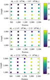 |
Fig. 12 Median NMSE on full hybrid signal for SCARF using different time segmentation strategies. The length of the last time segment |


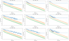 |
Fig. 13 Sliding NMSE for SCARF model and wavelet thresholding with threshold set as the chi2 critical value for p = 0.9 (SCARF in blue, wavelet re-weighted block thresholding in orange, wavelet thresholding in green). |
5 Conclusion and prospects
In this article, we have investigated different non-parametric approaches to detect and reconstruct MBHB signals from gravitational interferometric measurements, including wavelets and ML. To that end, we first investigated different models to represent MBHB waveforms on days-long time intervals, including sparse models based on wavelet representations and learning-based methods such as the PCA and the IAE. We assessed the limitations of these methods and proposed a hybrid method that combines the IAE to accurately represent the coalescence part of MBHB waveforms and an innovative adaptive STFT that adapts to the MBHB inspiral regime. We demonstrated how these approaches can be used to both detect MBHB waveforms, even at low S/N, and recover the MBHB signals.
One advantage of the hybrid method is that it is fast and can be extended to tackle more general signal processing tasks such as gap mitigation (i.e., inpainting) and signal unmixing. Furthermore, once the IAE model is trained and the SCARF parameters, no extra parameters are need to tackle detection and signal recovery. However, the current limitation of the proposed hybrid method is twofold. A first limitation could be the model’s sensitivity to the parameters of the SCARF transform. Nonetheless, we showed that the sensitivity depends on the MBHB chirp mass, which can be accurately derived from the coalescence. A second limitation, which is standard in ML-based signal representations, is model bias. This bias can be neglected when the noise level is large, but it can become large at high S/N. To overcome this issue, one standard approach could be to improve the IAE model by increasing the explicability or complexity of the model (e.g., more layers, more filters per layers, or using more generic architectures such as transformers), but this is at the cost of a more cumbersome training and the need for a larger training set. A second approach could be to hybridize both the IAE model of the coalescence with a wavelet-based representation, which is known to provide a vanishing bias when the noise decreases. In contrast to the non-parametric approach we investigated for GB, the proposed method builds upon a learning-based method that necessitates simulated MBHB waveforms at the training stage.
In this work, the method comparisons have been carried out based on detection and signal recovery performance, not MBHB parameter estimation. As stressed in Blelly et al. (2022), the proposed hybrid approach is quite general, and it will be used as a building block for more complex signal recovery tasks from gravitational interferometric measurements. It can be extended to tasks that are relevant for LISA, such as gap mitigation and, more generally, artifact mitigation (e.g., glitches) and the unmixing of gravitational events of similar or different nature. In addition, the proposed low-dimensional representations, such the IAE-based one, bears information about the parameters of the recovered MBHBs, which could be exploited as a first guess estimation in a Bayesian analysis framework.
Appendix A Whitening and filtering
Data pre-processing is operated by whitening and bandpass-ing the signal using the theoretical Power Spectrum Density of the noise defined in (Babak et al. 2021) as the noise variance at each frequency of the spectrum. For now, this noise is assumed gaussian and stationary but may evolve to address non-stationarity induced by fluctuations in LISA arm lengths and non-Gaussianity in the stochastic backgrounds.
The signal is also convolved with a Butterworth bandpass filter to mitigate the high LISA noise observed at low and high frequencies while gravitational signals remain around the milli-hertz frequency band. This results in multiplying the signal by the following gain in the frequency domain:
 (A.1)
(A.1)
with fmin set to 2.10−5Hz, fmax set to 5.10−2Hɀ and the order of the filter set to n = 4.
The result of this pre-processing is that noise can be considered white in the frequency range of interest and close to zero out of it.
Appendix B Simulated massive black hole binary generation
The fast generation of MBHB waveforms was performed using codes from lisabeta with parameters coherent with the LDC2a-Sangria data challenge.
The varying parameters in simulations were the chirp mass which was sampled logarithmically over the segment [5 · 105M⊙, 5 · 106M⊙], the mass ratio which was sampled linearly over [1, 3] and the initial phase sampled linearly over [0,2π].
The rest of the parameters were set to the value of the first MBHB in the LDC Sangria dataset and can be found in Table B.1. Since the waveforms are then multiplied by a scalar factor to get some chosen S/N values, the distance and angle do not give by themselves an accurate estimation of signal power, which is the controlled variable in the experiments. The sampling rate of the measurements is fixed to 5s.
MBHB waveform parameters.
Appendix C Interpolatory autoencoder architecture
The IAE model used in this article relies on ten anchor points picked from the training set to get a log-uniform sample of the chirp mass. Both encoder and decoder are 12 layer Convolutional Neural Networks. The filters used in the encoder and decoder CNN, as well as for the lateral connections between encoder and decoder are 1D convolution filters presented in Table C.1. This version of the IAE uses lateral connections to improve performance broadly based on an idea developed in (Rasmus et al. 2015). These lateral connections, described in Fig C.1, are composed of a layer in the encoder, an interpolation step and another layer in the decoder. To keep a coherent low-dimension representation, the interpolations in every lateral connection are set to share the same barycentric weights. When computing the barycentric weights associated to a waveform, the same weights are used in every lateral connection. The training loss of Eq 23 is then modified, summing the distance in each lateral connection with increasing weights moving away from the direct space.
The training loss used is a MSELoss and the activation function in the network is the ELU function (alpha=1). The training was performed on 10000 epochs, with batch size of 32 and learning rate of 0.001.
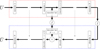 |
Fig. C.1 Description of the IAE architecture with focus on one lateral connection. The encoder (in red) is above the interpolation operators and the decoder under (in blue). Each layer is composed of the convolution filters described in Table C.1 and uses an Exponential Linear Unit (ELU) as the activation function. |
Appendix D SCARF
The SCARF time segmentation is based on a dyadic decomposition moving backward from coalescence with overlapping margins of 200 time samples on each sides. The associated windows are apodized using a squared sine to mitigate artefacts on the boundaries of the decomposition elements. Additionally, the decomposition is made overcomplete redundant segments covering the span between the middles of two consecutive windows as illustrated in Fig. D.1.
 |
Fig. D.1 Windowing strategy with segmentation, overlapping windows and apodization for the windows closest to merger |
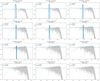 |
Fig. D.2 Example of SCARF decomposition of an MBHB and constrained thresholding associated, as windows get further from merger the peak drowns into noise but the propagation of information from higher S/N regions to lower ones help detect it in the latter |
References
- Abbott, B. P., Abbott, R., Abbott, T., et al. 2016, Phys. Rev. Lett., 116, 061102 [CrossRef] [PubMed] [Google Scholar]
- Amaro-Seoane, P., Audley, H., Babak, S., et al. 2017, arXiv e-prints [arXiv:1702.00786] [Google Scholar]
- Amaro-Seoane, P., Andrews, J., Arca Sedda, M., et al. 2023, Living Rev. Relativity, 26, 2 [NASA ADS] [CrossRef] [Google Scholar]
- Babak, S., Le Jeune, M., Petiteau, A., & Vallisneri, M. 2020, LISA Data Challenge: Sangria [Google Scholar]
- Babak, S., Hewitson, M., & Petiteau, A. 2021, arXiv e-prints [arXiv:2108.01167] [Google Scholar]
- Bacon, P., Gayathri, V., Chassande-Mottin, E., et al. 2018, Phys. Rev., D98, 024028 [NASA ADS] [Google Scholar]
- Bammey, Q., Bacon, P., Chassande-Mottin, E., Fraysse, A., & Jaffard, S. 2018, in 26th European Signal Processing Conference (EUSIPCO), IEEE, 1755 [Google Scholar]
- Bayle, J.-B. 2019, PhD thesis, Université de Paris; Université Paris Diderot; Laboratoire Astroparticules, France [Google Scholar]
- Bengio, Y., Courville, A., & Vincent, P. 2013, IEEE Trans. Pattern Anal. Mach. Intell., 35, 1798 [CrossRef] [Google Scholar]
- Blelly, A., Moutarde, H., & Bobin, J. 2020, Phys. Rev. D, 102, 104053 [CrossRef] [Google Scholar]
- Blelly, A., Bobin, J., & Moutarde, H. 2022, MNRAS, 509, 5902 [Google Scholar]
- Bobin, J., Gertosio, R. C., Bobin, C., & Thiam, C. 2023, Digital Signal Process., 139, 104058 [NASA ADS] [CrossRef] [Google Scholar]
- Cai, T. T. 1999, Ann. Statist., 27, 898 [CrossRef] [Google Scholar]
- Cai, J.-F., Candès, E. J., & Shen, Z. 2010, SIAM J. Optim., 20, 1956 [CrossRef] [Google Scholar]
- Candes, E. J., Wakin, M. B., & Boyd, S. P. 2008, J. Fourier Anal. Applic., 14, 877 [CrossRef] [Google Scholar]
- Chernogor, L. F., & Lazorenko, O. V. 2016, in 8th International Conference on Ultrawideband and Ultrashort Impulse Signals (UWBUSIS), IEEE, 47 [Google Scholar]
- Cornish, N. J., & Littenberg, T. B. 2015, Class. Quant. Grav., 32, 135012 [NASA ADS] [CrossRef] [Google Scholar]
- Duarte, M. F., & Eldar, Y. C. 2011, IEEE Trans. Signal Process., 59, 4053 [CrossRef] [Google Scholar]
- Elad, M., & Aharon, M. 2006, IEEE Trans. Image Process., 15, 3736 [CrossRef] [Google Scholar]
- Feng, F., Chassande-Mottin, E., Bacon, P., & Fraysse, A. 2018, in 26th European Signal Processing Conference (EUSIPCO) (Rome: IEEE), 1750 [CrossRef] [Google Scholar]
- Flandrin, P. 1999, Time-Frequency/Time-Scale Analysis (Laboratoire de Physique Ecole Normale Superieure Lyon) [Google Scholar]
- Gertosio, R. C., Bobin, J., & Acero, F. 2023, Signal Process., 202, 108776 [NASA ADS] [CrossRef] [Google Scholar]
- Goodfellow, I., Bengio, Y., & Courville, A. 2016, Deep Learning (MIT Press) [Google Scholar]
- Graff, C. G., & Sidky, E. Y. 2015, Appl. Opt., 54, C23 [NASA ADS] [CrossRef] [Google Scholar]
- Hampel, F. R., Ronchetti, E. M., Rousseeuw, P. J., & Stahel, W. A. 2011, Robust Statistics: The Approach Based on Influence Functions (John Wiley & Sons) [Google Scholar]
- Hinton, G. E., & Salakhutdinov, R. R. 2006, Science, 313, 504 [Google Scholar]
- Khan, S., Husa, S., Hannam, M., et al. 2016, Phys. Rev. D, 93 [Google Scholar]
- Klimenko, S., Yakushin, I., Rakhmanov, M., & Mitselmakher, G. 2004, Class. Quant. Grav., 21, S1685 [NASA ADS] [CrossRef] [Google Scholar]
- Kramer, M. A. 1991, AIChE J., 37, 233 [CrossRef] [Google Scholar]
- Marsat, S., & Baker, J. 2018, arXiv e-prints [arXiv:1806.10734] [Google Scholar]
- Morrás, G., Nuño Siles, J. F., & García-Bellido, J. 2023, Phys. Rev. D, 108, 123025 [CrossRef] [Google Scholar]
- Nie, F., Huang, H., Cai, X., & Ding, C. 2010, Adv. Neural Inform. Process. Syst., 23 [Google Scholar]
- Potter, L. C., Ertin, E., Parker, J. T., & Cetin, M. 2010, Proc. IEEE, 98, 1006 [CrossRef] [Google Scholar]
- Prince, T. A., Tinto, M., Larson, S. L., & Armstrong, J. W. 2002, Phys. Rev., D66, 122002 [NASA ADS] [Google Scholar]
- Rasmus, A., Berglund, M., Honkala, M., Valpola, H., & Raiko, T. 2015, Adv. Neural Inform. Process. Syst., 28 [Google Scholar]
- Robson, T., & Cornish, N. J. 2019, Phys. Rev., D99, 024019 [NASA ADS] [Google Scholar]
- Schmidt, S., Breschi, M., Gamba, R., et al. 2021, Phys. Rev. D, 103, 043020 [NASA ADS] [CrossRef] [Google Scholar]
- Starck, J.-L., Murtagh, F., & Fadili, M. 2010, Sparse Image and Signal Processing (Cambridge University Press) [CrossRef] [Google Scholar]
- Tinto, M., & Dhurandhar, S. V. 2014, Living Rev. Rel., 17, 6 [NASA ADS] [CrossRef] [Google Scholar]
- Tropp, J. A., & Wright, S. J. 2010, Proc. IEEE, 98, 948 [CrossRef] [Google Scholar]
- Wold, S., Esbensen, K., & Geladi, P. 1987, Chemometrics Intell. Lab. Syst., 2, 37 [CrossRef] [Google Scholar]
All Tables
All Figures
|
Fig. 1 Interpolatory autoencoder description. |
| In the text | |
|
Fig. 2 Different time-frequency tiling strategies and their respective efficiency at capturing an MBHB signal (represented in red). In a good sparse representation, the ratio of the number of active blocks over total blocks should be small. Furthermore, to increase the S/N within blocks and improve detectability, the ratio of the signal power over the block area should be high, especially early in the inspiral, where signal power is easily drowned in noise. |
| In the text | |
|
Fig. 3 Sketch of the SCARF time-frequency decomposition: the red block is the selected frequency segment on time bin , the candidates for time segments l – 1 are the ones with an upper bound among the green blocks, and the lower bound in the blue ones. The most powerful contiguous block are composed of elements that are each above threshold is selected as an active block on time segment l – 1 before moving back one time segment. |
| In the text | |
|
Fig. 4 Preprocessed (whitened and bandpassed) MBHB coalescences in time domain with noise (grey) and clean (blue) for different chirp masses and S/N. |
| In the text | |
|
Fig. 5 Reconstructed signals for the different methods at multiple chirp masses and S/N. The gray signal corresponds to the noisy input, the blue one to PCA reconstruction, the green one to wavelet reconstruction, and the orange one to the IAE reconstruction. |
| In the text | |
|
Fig. 6 Evolution of the median NMSE over S/N on signal extracted at merger. |
| In the text | |
|
Fig. 7 Scatter plots of the NMSE as a function of the chirp mass and mass ratio for different methods and S/N values. |
| In the text | |
|
Fig. 8 Detection histograms for PCA (12 norm statistic measured on pure noise in orange and on noisy signal in blue). |
| In the text | |
|
Fig. 9 Detection histograms for IAE (12 norm statistic measured on pure noise in orange and on noisy signal in blue). |
| In the text | |
|
Fig. 10 Detection histograms for wavelets (12 norm statistic measured on pure noise in orange and on noisy signal in blue). |
| In the text | |
|
Fig. 11 ROC curves at different S/N and chirp masses for PCA, IAE, and wavelet detection. |
| In the text | |
|
Fig. 12 Median NMSE on full hybrid signal for SCARF using different time segmentation strategies. The length of the last time segment |
| In the text | |
|
Fig. 13 Sliding NMSE for SCARF model and wavelet thresholding with threshold set as the chi2 critical value for p = 0.9 (SCARF in blue, wavelet re-weighted block thresholding in orange, wavelet thresholding in green). |
| In the text | |
|
Fig. C.1 Description of the IAE architecture with focus on one lateral connection. The encoder (in red) is above the interpolation operators and the decoder under (in blue). Each layer is composed of the convolution filters described in Table C.1 and uses an Exponential Linear Unit (ELU) as the activation function. |
| In the text | |
|
Fig. D.1 Windowing strategy with segmentation, overlapping windows and apodization for the windows closest to merger |
| In the text | |
|
Fig. D.2 Example of SCARF decomposition of an MBHB and constrained thresholding associated, as windows get further from merger the peak drowns into noise but the propagation of information from higher S/N regions to lower ones help detect it in the latter |
| In the text | |
Current usage metrics show cumulative count of Article Views (full-text article views including HTML views, PDF and ePub downloads, according to the available data) and Abstracts Views on Vision4Press platform.
Data correspond to usage on the plateform after 2015. The current usage metrics is available 48-96 hours after online publication and is updated daily on week days.
Initial download of the metrics may take a while.